Synthesizing Time-Series Gene Expression Data to Enhance Network Inference Performance Using Autoencoder

Abstract

It is a challenge to infer a gene regulatory network from time-series gene expression data in the systems biology field. A lack of gene expression data samples is a factor limiting the performance of the inference methods. To resolve this problem, we propose a novel autoencoder-based approach that synthesizes virtual gene expression data to be used as input to the inference method. Through intensive experiments, we showed that using synthetic gene expression as input improves the performance of the network inference method compared to that without it. In particular, the performance improvement was stable against the discretization level of gene expression, the number of time steps in the observed gene expression, and the number of genes.

1. Introduction

Gene regulatory networks (GRNs) describe the collective connections among genes, and they regulate their expressions. It is essential to clarify GRNs to understand the function of and disease in organisms. Thus, the inference of GRNs has been an important research topic [1], and many diverse methodologies, which are usually classified into model-free and model-based methods, have been developed. In model-free approaches, gene interactions can be identified by various statistical and machine learning techniques, including mutual information [2,3,4], random forests [5,6,7], or network deconvolution [8,9]. In model-based methodologies, a quantitative dynamical model is employed to represent the system’s dynamics, such as a Boolean network [10,11], an ordinary differential equation (ODE) [12,13,14,15], the regression method [16,17,18], or a dynamic Bayesian network (DBN) [19,20,21].

In the model-based inference methods, it is necessary to optimize the model parameters by using gene expression data. It is obvious that the data from longer observation times would help infer GRNs more accurately. However, time-series gene expression data is not always easily obtained [22]. In some cases, it may be difficult to ensure that observations are made under identical conditions throughout the observation period. Data augmentation has been considered as one of the effective approaches to resolve this data shortage problem. It has been frequently used in various domains such as image processing [23,24,25,26] and time-series prediction [27,28,29]. In the field of time-series gene expression, several strategies have also been proposed to generate artificial data, in particular, through the Dialogue on Reverse Engineering Assessment and Methods (DREAM) challenge [30,31]. Several previous investigations on this matter are accessible [32,33,34,35,36]. These studies can generate simulated biological datasets that closely mimic real-world data and provide researchers with tools to analyze and investigate genes. The artificial gene network (AGN) model is proposed to simulate temporal expression data for the identification of gene networks [37]. This model uses a feature selection technique where a specific gene remains constant, and the expression profiles of all other genes are observed. The goal is to identify a significant subset of predictors for the target gene. These studies proposed methods to produce synthetic data that closely resemble the real data. However, they have a limitation in producing a variety of data because they did not learn complex generation functions using data but tried to build simple rules. In particular, rule-based or manually designed simulations may fail to capture nonlinear or context-specific regulatory dynamics that naturally occur in biological systems. Additionally, these approaches often lack adaptability and may not generalize diverse datasets or unseen biological conditions.

In this study, we propose a network inference approach involving an autoencoder-based data generation model. For our problem, it is noteworthy that the autoencoder has some advantages over the generative adversarial network (GAN) [38]. The autoencoder provides a simple yet effective framework with a lightweight architecture that enables stable training by optimizing a single objective. On the other hand, the GAN requires simultaneous training of two competing networks, which causes mode collapse, sensitivity to hyperparameters, and instability during training [39,40]. Thus, the autoencoder is more suitable for gene expression problems, where available datasets are typically small and heterogeneous. Several studies have shown that autoencoders perform well in low-data regimes and can effectively extract meaningful representations in biological applications [41,42]. In addition, the performance of autoencoders is less dependent on the underlying distribution of gene expression values, allowing for better adaptability to biological variation. In this context, we utilize an autoencoder to learn a functional representation of gene expression dynamics from limited time-series data, generating additional synthetic samples to support more accurate network inference.

2. Materials and Methods

2.1. Discretized Network Model

In this study, we used a gene-wise discretized network model as presented in the previous study [43]. The discretized network can be modeled as a directed graph $G(V,A)$, where the vertex set $V=\{v_1,v_2,\dots ,v_N\}$ corresponds to N genes, and edges $A\subseteq V\times V$ encode regulatory interactions between them. The state of a gene v at time t, denoted as $v\left(t\right)$, assumes one of l discrete values from the set $\{0,1,2,\dots ,l-1\}$. When $l=2$ for all genes in V, the network is referred to as a Boolean network [44]. Suppose that $v\in V$ denotes a target node whose dynamics are governed by the interaction with k regulatory genes $u_1,u_2,\dots ,u_k$, where $u_i\in V$. Let E and $E_i$ denote the sets of possible discrete expression values for the gene v and the regulatory genes $u_i$, respectively. The state of v at the next time step, $v(t+1)$, is determined by a discrete function $f:E_1\times E_2\times \dots \times E_k\to E$, which maps the expression values of the k regulatory genes at time t to an updated state. Consequently, the update rule for v can be expressed as follows:

$$v(t+1)=f(u_1\left(t\right),u_2\left(t\right),...,u_k\left(t\right)).$$

In this study, we adopted an update time lag of one. The total number of possible functions f is given by $l^{{\prod }_i{l}_i}$, where $l=\left|E\right|$ and $l_i=\left|E_i\right|$ denote the cardinalities of the sets E and $E_i$, respectively.

2.2. Network Inference Problem

In this study, we addressed the problem of network inference from time-series gene expression data, aiming to recover both the regulatory interactions and their associated update functions. The quality of the inferred network was evaluated by comparing the trajectories it generates with those observed in the original time-series data. Let ${\mathbf{v}}^{\prime }=[v^{\prime }\left(1\right),v^{\prime }\left(2\right),...,v^{\prime }\left(T\right)]$ denote the sequence of the predicted expression states of gene v for a time step ranging from 1 to T, based on the inferred discretized network. Then, the dynamic accuracy of the inferred network is defined as follows:

$$DynamicAccuracy={\displaystyle \frac{1}{N·T}}\sum _{i=1}^N\sum _{t=1}^T(1-D\left({\mathbf{v}}^{\prime },\mathbf{v}\right)),$$

where T denotes the total number of time points and $D\left({\mathbf{v}}^{\prime },\mathbf{v}\right)$ is the Hamming distance between two sequences of ${\mathbf{v}}^{\prime }$ and $\mathbf{v}$.

2.3. Structural Performance Metrics

In this study, we employed three well-known evaluation metrics, namely precision, recall, and structural accuracy to quantify the structural similarity between the inferred and the corresponding ground truth networks. Precision measures the proportion of correctly inferred regulatory connections ($TP$) among all predicted ones ($AP$) and is defined as follows:

$$Precision={\displaystyle \frac{TP}{AP}}.$$

Recall quantifies the proportion of correctly inferred connections ($TP$) over the whole number of connections (P) and is defined as follows:

$$Recall={\displaystyle \frac{TP}{P}}.$$

Finally, structural accuracy assesses the proportion of true positive and negative predictions ($TP$ and $TN$) out of all positive and negative connections (P and N) and is defined as follows:

$$StructuralAccuracy={\displaystyle \frac{TP+TN}{P+N}}.$$

2.4. Network Inference Method

In this study, we synthesized time-series discrete expression data to improve the existing network inference method. To this end, we used mutual information based on multiple-level discretization network inference (MIDNI) [43]. The latter is an algorithm developed from the mutual information-based Boolean network inference method (MIBNI) [45]. The former reconstructs the discrete network by properly discretizing gene expression values into two or three levels depending on their distribution, whereas the latter infers the Boolean network based on the binarized gene expression values. This higher degree of freedom in expression led to more accurate inference results in MIDNI.

2.5. Autoencoder Model

The concept of an autoencoder was originally proposed by LeCun in 1987 [46]. It is an artificial neural network designed to acquire efficient representations of input data, primarily for dimensionality reduction or feature extraction. It comprises two components, namely an encoder and a decoder. The encoder compresses the input data into a reduced-dimensional representation, referred to as the “latent space” or “code”, whereas the decoder utilizes the compressed latent representation to recreate the original input data with maximal fidelity. Since it was invented, numerous autoencoder variations have been effectively used in a variety of domains, including natural language processing [47,48,49], computer vision [50,51,52], and speech recognition [53,54]. In our study, we employed a conventional autoencoder with a reasonable number of hidden layers to achieve a compromise between efficiency and training duration [55,56]. Unlike traditional autoencoders that aim to reconstruct the input data itself, the proposed model is trained to predict the next state $v(t+1)$ given the current state $v\left(t\right)$ as input. This architecture retains the encoder–decoder structure, but the training objective shifts from input reconstruction to temporal state prediction. It seeks to reduce the discrepancy between the actual and predicted values by minimizing the loss function. By learning a compressed latent representation of $v\left(t\right)$ that captures temporal dynamics, the decoder is optimized to generate the corresponding $v(t+1)$ rather than reproducing $v\left(t\right)$. While the model may produce diverse gene expression profiles due to the limited dataset, this variation is consistent with natural biological variability. Instead of evaluating the biological plausibility of the synthetic data directly, we assess its utility through downstream network inference, interpreting the successful reconstruction of gene regulatory networks as an indirect yet meaningful indicator of data quality.

3. Our Proposed Method

Figure 1 shows the entire framework of our approach. An observed discrete gene expression dataset is given as an input. It is represented by a K × N discrete matrix, where K and N indicate the number of observed time steps and genes, respectively. The matrix is used to generate two other discrete matrices of $(K-1)$ × N size, which are input–target pair matrices. They establish a relationship between consecutive network states, which will be learned by the autoencoder. The learned autoencoder can synthesize gene expression values after the observed time steps. The synthesized and observed discretized gene expressions are combined into a single matrix, and this is used as input for the inference algorithm MIDNI. Each part of our approach is explained in detail in the next subsections.

3.1. Synthesis of Gene Expression

The given input data is an observed, discretized gene expression matrix of $K\times N$ size. Let $\mathbf{v}\left(t\right)=[v_1\left(t\right),v_2\left(t\right),...,v_N\left(t\right)]$ be a network state at time step t represented by a vector of all gene values. Then, the input data are the collection of $\mathbf{v}\left(t\right)$ for all observed time steps ($t=1,2,$...$,K$). The observed gene expression matrix is transformed into two $(K-1)\times N$ matrices called the input and target matrices for training the autoencoder. The first and second matrices are the collections of $\mathbf{v}\left(t\right)$ ranging from $t=1$ to $t=K-1$ and from $t=2$ to $t=K$, respectively. This representation can delineate the correlation of gene expression values between two consecutive time steps, enabling the autoencoder to effectively identify the underlying dynamics. After the training process is finished, the autoencoder model can be used to generate unobserved discrete gene expression data after the last observation time step K. At the first iteration of the generation process, $\mathbf{v}\left(K\right)$, the network state at the last observation time step is given as an input to the model, and the model produces an output ${\mathbf{v}}^{\prime }(K+1)$, which is used as an input for the output ${\mathbf{v}}^{\prime }(K+2)$ and so on. This process is repeated for a desired time step. The structure of the autoencoder is presented in

Table 1. The structure of the autoencoder model.

Parameter’s Name	Value
Dimension of the input layer	N
Dimension of the output layer	N
Number of hidden layers	3
Number of neurons in the first hidden layer	$2\times N$
Number of neurons in the second hidden layer	512
Number of neurons in the third hidden layer	$2\times N$
Activation function in hidden layers	relu
Activation function in the output layer	linear

. We chose the set of parameters that provides the best results, as presented in

Table 2. Parameters of the training.

Parameter’s Name	Value
Model optimizer	Adam
Learning rate	0.001–0.01 *
Loss function	mse
Number of epochs	1000–10,000 *
Batch size	32

* The values are different depending on the size of the input network.

. The model structure and hyperparameters were selected through extensive empirical tuning considering the specific characteristics of biological gene expression data and the demands of network reconstruction tasks. A symmetric three-layer architecture was chosen to provide sufficient capacity for capturing the complex nonlinear relationships commonly observed in gene regulatory networks while avoiding overfitting typically observed in small biological datasets. ReLU activation functions were used in the hidden layers due to their ability to efficiently learn sparse representations. This aligns with the biological assumption that only a subset of genes is co-regulated at a time. In contrast, alternatives like sigmoid and tanh introduced saturation effects and slower convergence. Linear output activation preserves the full dynamic range of gene expression values (between 0 and 2). The learning rate and training epochs were dynamically adjusted to accommodate datasets of varying size and complexity, ensuring stable convergence without sacrificing generalization. These design choices were made to optimize the model’s ability to generate biologically plausible data and support the accurate inference of regulatory interactions.

3.2. Inference of GRN

As mentioned in Section 2.4, we applied MIDNI to the synthesized discrete gene expression data. Two key parameters are configured for MIDNI in this study: First, the time lag parameter is set to one, that is to say, the expression of a regulator gene at time step t influences the expression of its target gene at time step $(t+1)$. The time lag accounts for the inherent delays in biological processes, such as transcription, translation, and the diffusion of regulatory molecules, which are essential for accurately capturing the dynamic nature of gene regulatory interactions. Second, the maximum number of regulators is set to five. This constraint reduces the computational complexity of the network inference process while maintaining biological relevance such that most genes are regulated by a relatively small number of key regulators in real biological systems.

4. Experimental Results

4.1. Experiment Setup

To comprehensively evaluate the performance and robustness of our proposed method, we conducted experiments on synthetic datasets representing gene regulatory networks (GRNs) of two different network sizes $N=50$ and $N=100$. These sizes were chosen to reflect small-to-intermediate complex biological systems, allowing us to examine the scalability of our method under different conditions. For each network size, we generated 10 structurally distinct ground truth networks using the Barabási–Albert (BA) model [57], which is a widely used generative model that captures the scale-free properties commonly observed in real-world biological networks. This resulted in a total of 20 unique ground truth networks used in our experiments. For each ground truth network, we simulated discretized gene expression data over K observed time steps using a dynamic model outlined in Algorithms S1 and S2 (see Supplementary Materials). These simulated time-series datasets serve as the foundation for evaluating our method’s ability to infer network structure from temporal gene expression patterns. Two levels of discretization were considered to reflect different degrees of resolution in experimental measurements, namely binary (two states: 0 or 1) and ternary (three states: 0, 1, or 2). This allowed us to assess the method’s sensitivity and effectiveness across datasets with varying levels of granularity. Our method takes the observed gene expression data over the initial K time steps as input and synthesizes the gene expression values for the remaining $(T-K)$ time steps, where the total length of the time-series is fixed at $T=100$. The ability to generate synthetic future data is a critical component of our approach, as it allows us to enrich the dataset and potentially improve inference accuracy, especially in cases where only a limited number of observations are available. To systematically investigate the influence of the number of observed time steps on inference performance, we varied K from 10 to 90 in increments of 10. This setup enables us to explore how the quantity of available temporal data affects both the quality of synthetic data generation and the subsequent network inference. We applied the network inference algorithm, MIDNI, to both the original and synthesized datasets. The inferred networks were then compared against the corresponding ground truth networks using the evaluation metrics explained in Section 2.3. Performance was analyzed separately for datasets discretized into ternary levels (see Figure 2) and binary levels (see Figure 3). Comprehensive results are provided in Tables S1 and S2 (see Supplementary Materials). These comparisons provide insight into how well our method reconstructs the underlying network structure under different data conditions and discretization schemes.

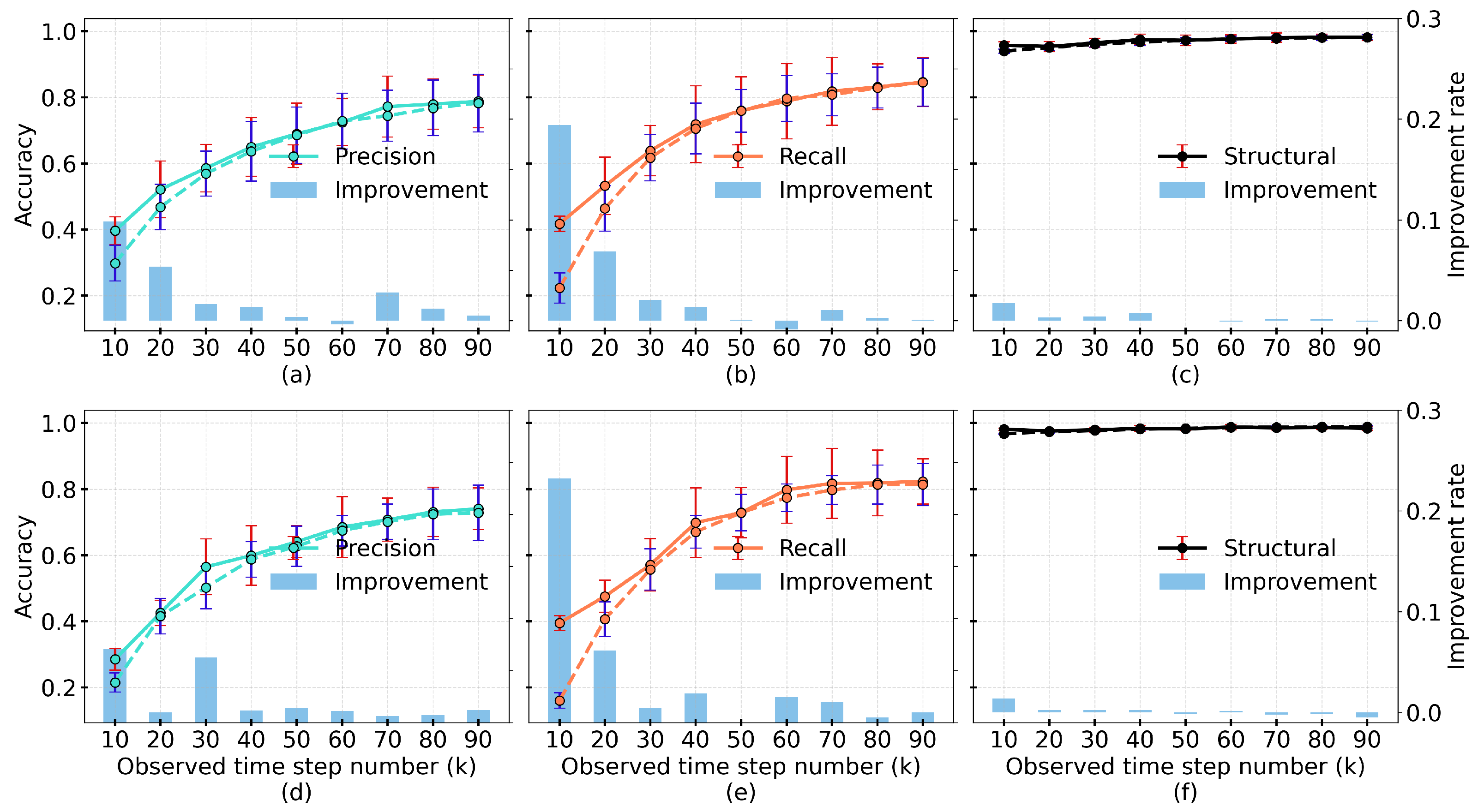
4.2. Results of Structural Performance

As shown in Figure 2a (see Table S1 in the Supplementary Materials for details), the precision values of the networks inferred based on the original data (dashed line) and the synthetic data (solid line) continuously increase as the observed time steps (K) increase in the networks with $\left|V\right|=50$. This is because the more expression data used for the inference algorithm, the higher the inference performance. The precision improvement by the use of the synthetic data was observed in all K values except for $K=60$ and 90. In addition, we can observe a similar trend with respect to the recall performance (Figure 2b). In particular, the degree of the performance improvement at $K=10$ was significantly larger. These observations indicate that the precision improvement by the synthetic data is not by reducing the number of positive predictions of interactions but by predicting the true positive interactions more accurately. Although the synthetic data also improved the structural accuracy, the improvement was not significant (Figure 2c). This is because the number of true negatives is much larger than that of true positives. We note that these findings were consistently observed in the networks with a larger network size ($\left|V\right|=100$) (Figure 2d–f). Taken together, our synthetic approach can be considerably useful when the observation time of the gene expression is limited in the real experimental environment.

We also investigated our method with respect to the Boolean networks, as shown in Figure 3 (see Table S2 in the Supplementary Materials for details). As in the ternary network results, we can observe the performance improvement of precision, recall, and structural accuracy in most cases. This means that our method is also effective in the Boolean network models. It is interesting that the recall improvement by our method was relatively larger on average than the precision improvement in the case of $\left|V\right|=50$, whereas the latter was relatively larger than the first in the case of $\left|V\right|=100$. This is because the MIDNI algorithm cannot control the number of positive predictions. However, we note that there is no negative influence on any performance measure. It is also interesting that the performance improvement does not increase as the observation time step K increases. For example, the precision was highest when K is 60 and 50 in the networks of $\left|V\right|=50$ and $\left|V\right|=100$, respectively (Figure 3a,d), and the recall was highest at $K=70$ in the networks of $\left|V\right|=100$ (Figure 3e). These results mean that the desirable number of observation time steps is dependent on the degree of discretization levels.

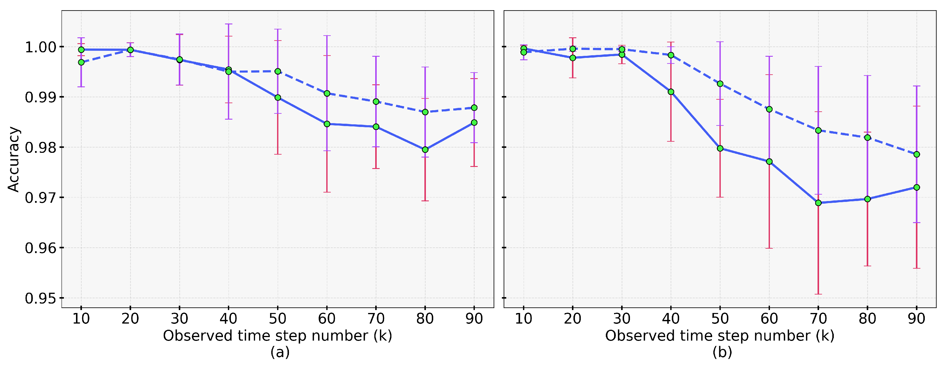
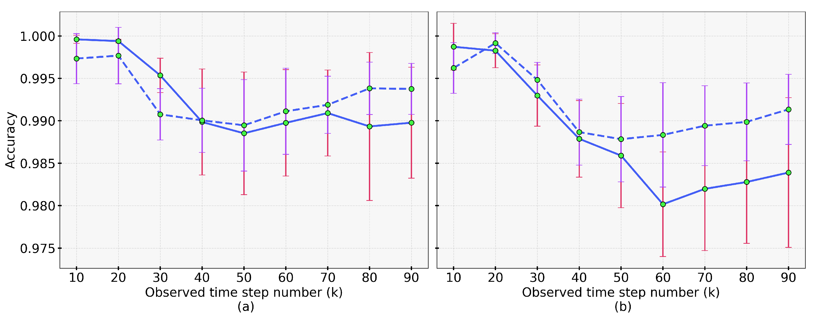
4.3. Results of Dynamic Accuracy

We also evaluated the dynamic accuracy of both the networks inferred from the original and the synthetic data on the multi-level discretization dataset (Figure 4) and on the Boolean discretization dataset (Figure 5). Contrary to precision or recall metrics, the dynamic accuracy tends to decrease as the number of time steps increases. We believe this is due to the increase in the number of data samples to be fitted by the inferred network. Moreover, the incorporation of additional time points may introduce deviations from the patterns already learned by the model, particularly if the new data include noise, nonlinear dynamics, or previously unobserved system behaviors. In addition, the dynamic accuracy of the synthetic data-driven networks is inferior to that of the original data-driven networks in most cases. We note that the latter is investigated over K time steps, whereas the former is investigated over T time steps, which is longer than K. Considering this difference between the examination time steps, the performance difference in terms of the dynamics accuracy may not be considerably significant.

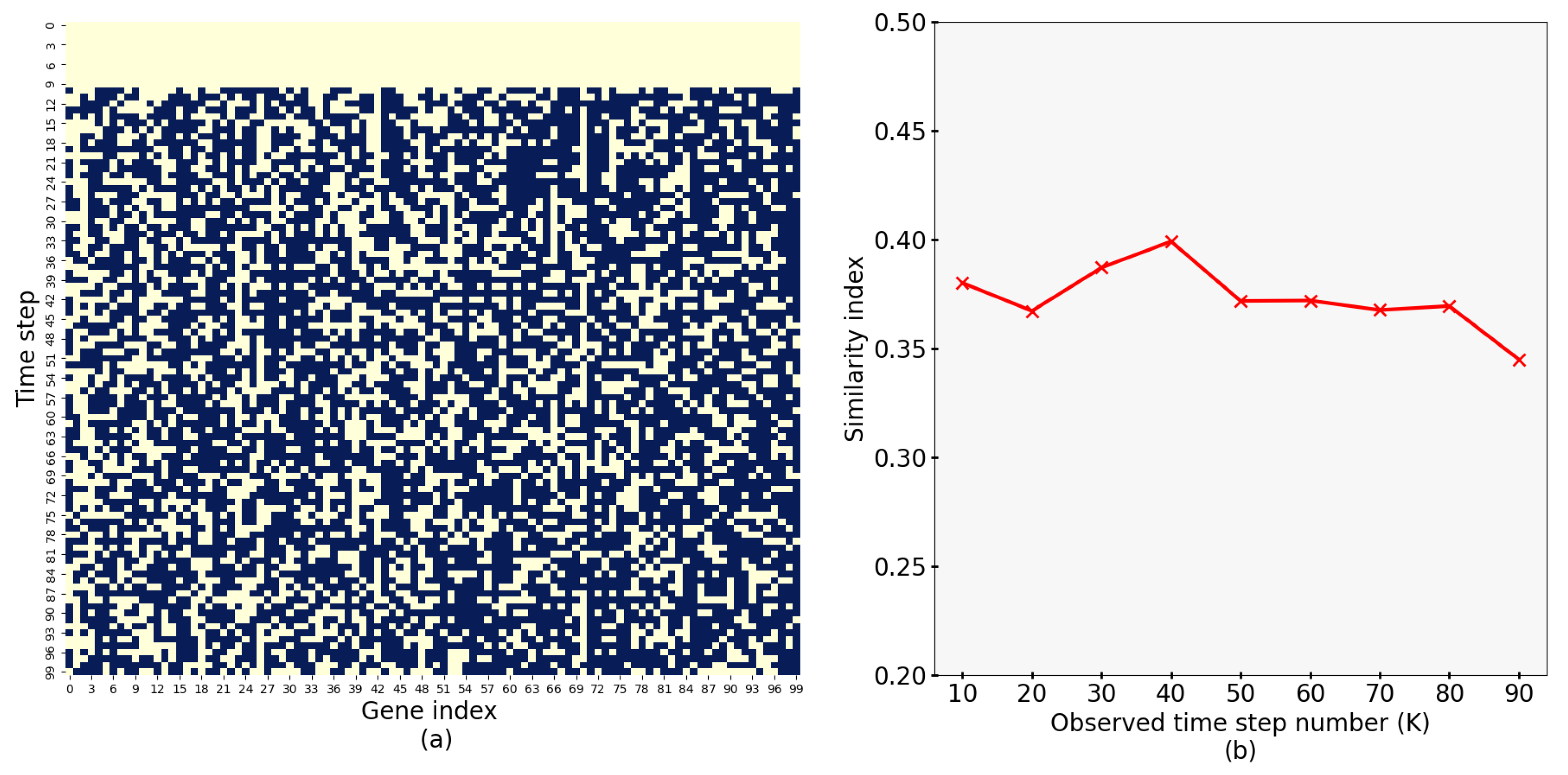
4.4. Results of Similarity of Synthesized Expressions

The autoencoder can generate the gene expression data differently whenever it is executed. To investigate how much the synthesized data are varied, we first created a random ground truth network with $N=100$ and generated an original ternary gene expression with K time steps ranging from 10 to 90 (see Algorithm S2 in the Supplementary Materials). For each K, we trained an autoencoder using the original gene expression and generated three different synthetic gene expressions for later $=T-K$ time steps. For three pairs of the gene expression matrices of $T\times N$ size, we investigated the similarity matrix, where the white and the black dots represent whether the corresponding gene expression values in the pair matrices are identical or not, respectively (Figure 6). As shown in the figure, the synthesized gene expressions are significantly different from each other. However, the inference performance based on these synthetic data is not significantly different. In other words, the autoencoder model produces diverse synthesized expressions but induces stable performance.

5. Discussion and Conclusions

In this study, we used an autoencoder model to synthesize gene expression data to overcome data scarcity problems in reverse engineering. Specifically, it produces additional time-series expression data to complement the observed gene expression data. The synthesized gene expression data were assessed using an inference algorithm. The experimental results demonstrated that the inference performance using synthetic gene expression was consistently higher than that using only the observed gene expression. This finding substantiates the effectiveness of the proposed model as a valuable tool for addressing network inference problems, particularly when there is a limitation in obtaining gene expression data of a sufficiently long observation time.

Furthermore, as gene expression data inherently possess structural relationships among genes, future work could explore the integration of graph representation learning techniques as a complementary or alternative approach. These methods are well-suited for modeling structured biological systems and may improve the quality of synthetic data or enhance network inference performance by capturing complex topological patterns in gene regulatory networks [58,59]. Another future study could be to extend the current framework based primarily on discretized gene expression data to operate directly on continuous-valued datasets. The reliance on discretization introduces variability due to method-specific assumptions, potentially affecting inference outcomes. Developing a discretization-free approach would increase the generalizability of the method. Additionally, integrating more advanced generative models such as GANs may further improve the diversity and biological realism of the synthesized data. Finally, a comprehensive validation of real-world biological datasets will be essential to evaluate the robustness and practical utility of the proposed method across diverse application scenarios, including rare disease modeling and temporal transcriptomic analyses.

References

1. Malvina, M.; Pancaldi, V. From time-series transcriptomics to gene regulatory networks: A review on inference methods. PLoS Comput. Biol. 2023, 19, e1011254. [Google Scholar]
2. Margolin, A.A.; Nemenman, I.; Basso, K.; Wiggins, C.; Stolovitzky, G.; Favera, R.D.; Califano, A. ARACNE: An Algorithm for the Reconstruction of Gene Regulatory Networks in a Mammalian Cellular Context. BMC Bioinform. 2006, 7 (Suppl. 1), S7. [Google Scholar] [CrossRef] [PubMed]
3. Yang, B.; Xu, Y.; Maxwell, A.; Koh, W.; Gong, P.; Zhang, C. MICRAT: A novel algorithm for inferring gene regulatory networks using time series gene expression data. BMC Syst. Biol. 2018, 12, 19–29. [Google Scholar] [CrossRef]
4. Liang, K.; Wang, X. Gene regulatory network reconstruction using conditional mutual information. EURASIP J. Bioinform. Syst. Biol. 2008, 2008, 253894. [Google Scholar] [CrossRef]
5. Huynh-Thu, V.A.; Irrthum, A.; Wehenkel, L.; Geurts, P. Inferring regulatory networks from expression data using tree-based methods. PLoS ONE 2010, 5, e12776. [Google Scholar] [CrossRef]
6. Petralia, F.; Wang, P.; Yang, J.; Tu, Z. Integrative random forest for gene regulatory network inference. Bioinformatics 2015, 31, i197–i205. [Google Scholar] [CrossRef]
7. Park, S.; Kim, J.M.; Shin, W.; Han, S.W.; Jeon, M.; Jang, H.J.; Jang, I.S.; Kang, J. BTNET: Boosted tree-based gene regulatory network inference algorithm using time-course measurement data. BMC Syst. Biol. 2018, 12, 20. [Google Scholar] [CrossRef] [PubMed]
8. Chen, H.; Mundra, P.A.; Zhao, L.N.; Lin, F.; Zheng, J. Highly sensitive inference of time-delayed gene regulation by network deconvolution. BMC Syst. Biol. 2014, 8, S6. [Google Scholar] [CrossRef] [PubMed]
9. Siegal-Gaskins, D.; Ash, J.N.; Crosson, S. Model-based deconvolution of cell cycle time-series data reveals gene expression details at high resolution. PLoS Comput. Biol. 2009, 5, e1000460. [Google Scholar] [CrossRef]
10. Trinh, H.C.; Kwon, Y.K. A novel constrained genetic algorithm-based Boolean network inference method from steady-state gene expression data. Bioinformatics 2021, 37 (Suppl. 1), i383–i391. [Google Scholar] [CrossRef]
11. Hickman, G.J.; Hodgman, T.C. Inference of gene regulatory networks using boolean-network inference methods. J. Bioinform. Comput. Biol. 2009, 7, 1013–1029. [Google Scholar] [CrossRef] [PubMed]
12. Ma, B.; Fang, M.; Jiao, X. Inference of gene regulatory networks based on nonlinear ordinary differential equations. Bioinformatics 2020, 36, 4885–4893. [Google Scholar] [CrossRef] [PubMed]
13. Li, Z.; Li, P.; Krishnan, A.; Liu, J. Large-scale dynamic gene regulatory network inference combining differential equation models with local dynamic Bayesian network analysis. Bioinformatics 2011, 27, 2686–2691. [Google Scholar] [CrossRef] [PubMed]
14. Aalto, A.; Viitasaari, L.; Ilmonen, P.; Mombaerts, L.; Gonçalves, J. Gene regulatory network inference from sparsely sampled noisy data. Nat. Commun. 2020, 11, 3493. [Google Scholar] [CrossRef]
15. Bin, Y.; Chen, Y. Overview of gene regulatory network inference based on differential equation models. Curr. Protein Pept. Sci. 2020, 21, 1054–1059. [Google Scholar]
16. Thorne, T. Approximate inference of gene regulatory network models from RNA-Seq time series data. BMC Bioinform. 2018, 19, 127. [Google Scholar] [CrossRef]
17. Michailidis, G.; d’Alché-Buc, F. Autoregressive models for gene regulatory network inference: Sparsity, stability and causality issues. Math. Biosci. 2013, 246, 326–334. [Google Scholar] [CrossRef]
18. Breiman, L. Random forests. Mach. Learn. 2001, 45, 5–32. [Google Scholar] [CrossRef]
19. Murphy, K.; Mian, S. Modelling Gene Expression Data Using Dynamic Bayesian Networks; Technical Report; Computer Science Division, University of California: Berkeley, CA, USA, 1999. [Google Scholar]
20. Kim, S.Y.; Imoto, S.; Miyano, S. Inferring gene networks from time series microarray data using dynamic Bayesian networks. Brief. Bioinform. 2003, 4, 228–235. [Google Scholar] [CrossRef]
21. Zou, M.; Conzen, S.D. A new dynamic Bayesian network (DBN) approach for identifying gene regulatory networks from time-course microarray data. Bioinformatics 2005, 21, 71–79. [Google Scholar] [CrossRef]
22. Murphy, D. Gene expression studies using microarrays: Principles, problems, and prospects. Adv. Physiol. Educ. 2002, 26, 256–270. [Google Scholar] [CrossRef] [PubMed]
23. Waqas, N.; Safie, S.I.; Kadir, K.A.; Khan, S.; Khel, M.H.K. DEEPFAKE Image Synthesis for Data Augmentation. IEEE Access 2022, 10, 80847–80857. [Google Scholar] [CrossRef]
24. Frid-Adar, M.; Klang, E.; Amitai, M.; Goldberger, J.; Greenspan, H. Synthetic data augmentation using GAN for improved liver lesion classification. In Proceedings of the 2018 IEEE 15th International Symposium on Biomedical Imaging (ISBI 2018), Washington, DC, USA, 4–7 April 2018; pp. 289–293. [Google Scholar] [CrossRef]
25. Zhang, Y.; Wang, Q.; Hu, B. MinimalGAN: Diverse medical image synthesis for data augmentation using minimal training data. Appl. Intell. 2023, 53, 3899–3916. [Google Scholar] [CrossRef]
26. Shin, H.C.; Tenenholtz, N.A.; Rogers, J.K.; Schwarz, C.G.; Senjem, M.L.; Gunter, J.L.; Andriole, K.P.; Michalski, M. Medical Image Synthesis for Data Augmentation and Anonymization Using Generative Adversarial Networks. In Simulation and Synthesis in Medical Imaging; Gooya, A., Goksel, O., Oguz, I., Burgos, N., Eds.; SASHIMI 2018; Lecture Notes in Computer Science; Springer: Cham, Switzerland, 2018; Volume 11037. [Google Scholar] [CrossRef]
27. Forestier, G.; Petitjean, F.; Dau, H.A.; Webb, G.I.; Keogh, E. Generating Synthetic Time Series to Augment Sparse Datasets. In Proceedings of the 2017 IEEE International Conference on Data Mining (ICDM), New Orleans, LA, USA, 9–12 December 2017; pp. 865–870. [Google Scholar] [CrossRef]
28. Maweu, B.M.; Shamsuddin, R.; Dakshit, S.; Prabhakaran, B. Generating Healthcare Time Series Data for Improving Diagnostic Accuracy of Deep Neural Networks. IEEE Trans. Instrum. Meas. 2021, 70, 2508715. [Google Scholar] [CrossRef]
29. Leznik, M.; Michalsky, P.; Willis, P.; Schanzel, B.; Östberg, P.O.; Domaschka, J. Multivariate Time Series Synthesis Using Generative Adversarial Networks. In Proceedings of the ACM/SPEC International Conference on Performance Engineering, ICPE ’21, New York, NY, USA, 19–23 April 2021; pp. 43–50. [Google Scholar] [CrossRef]
30. Schaffter, T.; Marbach, D.; Floreano, D. GeneNetWeaver: In silico benchmark generation and performance profiling of network inference methods. Bioinformatics 2011, 27, 2263–2270. [Google Scholar] [CrossRef]
31. DREAM. Dream: Dialogue for Reverse Engineering Assessments and Methods. 2009. Available online: https://gnw.sourceforge.net/dreamchallenge.html (accessed on 15 November 2010).
32. Albert, I.; Thakar, J.; Li, S.; Zhang, R.; Albert, R. Boolean network simulations for life scientists. Source Code Biol. Med. 2008, 3, 16. [Google Scholar] [CrossRef]
33. de Jong, H. Modeling and simulation of genetic regulatory systems: A literature review. J. Comput. Biol. 2002, 9, 67–103. [Google Scholar] [CrossRef]
34. De Jong, H.; Geiselmann, J.; Hernandez, C.; Page, M. Genetic Network Analyzer: Qualitative simulation of genetic regulatory networks. Bioinformatics 2003, 19, 336–344. [Google Scholar] [CrossRef]
35. Mendes, P.; Sha, W.; Ye, K. Artificial gene networks for objective comparison of analysis algorithms. Bioinformatics 2003, 19 (Suppl. 2), ii22–ii29. [Google Scholar] [CrossRef]
36. Van den Bulcke, T.; Van Leemput, K.; Naudts, B.; van Remortel, P.; Ma, H.; Verschoren, A.; De Moor, B.; Marchal, K. SynTReN: A generator of synthetic gene expression data for design and analysis of structure learning algorithms. BMC Bioinform. 2006, 7, 43. [Google Scholar] [CrossRef]
37. Martins Lopes, F.; Marcondes, R.M., Jr.; da Fontaura Costa, L. Gene expression complex networks: Synthesis, identification, and analysis. J. Comput. Biol. 2011, 18, 1353–1367. [Google Scholar] [CrossRef] [PubMed]
38. Goodfellow, I.; Pouget-Abadie, J.; Mirza, M.; Xu, B.; Warde-Farley, D.; Ozair, S.; Courville, A.; Bengio, Y. Generative adversarial networks. Commun. ACM 2020, 63, 139–144. [Google Scholar] [CrossRef]
39. Arjovsky, M.; Bottou, L. Towards Principled Methods for Training Generative Adversarial Networks. arXiv 2017, arXiv:1701.04862. [Google Scholar] [CrossRef]
40. Salimans, T.; Goodfellow, I.; Zaremba, W.; Cheung, V.; Radford, A.; Chen, X. Improved Techniques for Training GANs. arXiv 2016, arXiv:1606.03498. [Google Scholar] [CrossRef]
41. Tan, J.; Ung, M.; Cheng, C.; Greene, C.S. Unsupervised feature construction and knowledge extraction from genome-wide assays of breast cancer with denoising autoencoders. Pac. Symp. Biocomput. 2015, 20, 132–143. [Google Scholar] [PubMed] [PubMed Central]
42. Chen, L.; Cai, C.; Chen, V.; Lu, X. Learning a hierarchical representation of the yeast transcriptomic machinery using an autoencoder model. BMC Bioinform. 2016, 17 (Suppl. 1), S9. [Google Scholar] [CrossRef]
43. Anh, C.-T.; Kwon, Y.-K. Mutual Information Based on Multiple Level Discretization Network Inference from Time Series Gene Expression Profiles. Appl. Sci. 2023, 13, 11902. [Google Scholar] [CrossRef]
44. Kauffman, S.A. Gene regulation networks: A theory for their structure and global behavior. In Current Topics in Developmental Biology 6; Moscana, A., Monroy, A., Eds.; Academic Press: New York, NY, USA, 1971; pp. 145–182. [Google Scholar] [CrossRef]
45. Barman, S.; Kwon, Y.-K. A novel mutual information-based Boolean network inference method from time-series gene expression data. PLoS ONE 2017, 12, e0171097. [Google Scholar] [CrossRef]
46. LeCun, Y. Connexionist Learning Models. Ph.D. Thesis, Sorbonne University—Pierre and Marie Curie Campus, Paris, France, 1987. [Google Scholar]
47. Li, J.; Luong, M.; Jurafsky, D. A Hierarchical Neural Autoencoder for Paragraphs and Documents. arXiv 2015, arXiv:1506.01057. [Google Scholar] [CrossRef]
48. Freitag, M.; Roy, S. Unsupervised Natural Language Generation with Denoising Autoencoders. arXiv 2018, arXiv:1804.07899. [Google Scholar] [CrossRef]
49. Akram, M.W.; Salman, M.; Bashir, M.F.; Salman, S.M.S.; Gadekallu, T.R.; Javed, A.R. A novel deep auto-encoder based linguistics clustering model for social text. ACM Trans. Asian-Low-Resour. Lang. Inf. Process. 2022. [Google Scholar] [CrossRef]
50. Zhou, Z.; Liu, X. Masked Autoencoders in Computer Vision: A Comprehensive Survey. IEEE Access 2023, 11, 113560–113579. [Google Scholar] [CrossRef]
51. Parmar, G.; Li, D.; Lee, K.; Tu, Z. Dual contradistinctive generative autoencoder. In Proceedings of the IEEE/CVF Conference on Computer Vision and Pattern Recognition, Nashville, TN, USA, 20–25 June 2021; pp. 823–832. [Google Scholar] [CrossRef]
52. Cheng, Z.; Sun, H.; Takeuchi, M.; Katto, J. Deep convolutional autoencoder-based lossy image compression. In Proceedings of the 2018 Picture Coding Symposium (PCS), San Francisco, CA, USA, 24–27 June 2018; pp. 253–257. [Google Scholar] [CrossRef]
53. Vachhani, B.; Bhat, C.; Das, B.; Kopparapu, S.K. Deep Autoencoder Based Speech Features for Improved Dysarthric Speech Recognition. In Interspeech; ISCA: Stockholm, Sweden, 2017; pp. 1854–1858. [Google Scholar]
54. Karita, S.; Watanabe, S.; Iwata, T.; Delcroix, M.; Ogawa, A.; Nakatani, T. Semi-supervised end-to-end speech recognition using text-to-speech and autoencoders. In Proceedings of the ICASSP 2019-2019 IEEE International Conference on Acoustics, Speech and Signal Processing (ICASSP), Brighton, UK, 12–17 May 2019; pp. 6166–6170. [Google Scholar] [CrossRef]
55. Géron, A. Hands-On Machine Learning with Scikit-Learn, Keras, and TensorFlow; O’Reilly Media; 2022; ISBN 9781098122478. Available online: https://books.google.co.kr/books?id=V5ySEAAAQBAJ (accessed on 4 October 2022).
56. Song, Q.; Jin, H.; Hu, X. Automated Machine Learning in Action; Manning Publications; 2022; ISBN 9781617298059. Available online: https://www.manning.com/books/automated-machine-learning-in-action (accessed on 7 June 2022).
57. Barabási, A.-L.; Albert, R. Emergence of Scaling in Random Networks. In The Structure and Dynamics of Networks; Princeton University Press: Princeton, NJ, USA, 2006; pp. 349–352. [Google Scholar] [CrossRef]
58. Chen, F.; Wang, Y.-C.; Wang, B.; Kuo, C.-C.J. Graph representation learning: A survey. Apsipa Trans. Signal Inf. Process. 2020, 9, e15. [Google Scholar] [CrossRef]
59. Li, G.; Zhao, B.; Su, X.; Yang, Y.; Hu, P.; Zhou, X.; Hu, L. Discovering Consensus Regions for Interpretable Identification of RNA N6-Methyladenosine Modification Sites via Graph Contrastive Clustering. IEEE J. Biomed. Health Inform. 2024, 28, 2362–2372. [Google Scholar] [CrossRef] [PubMed]
Figure 1. The framework of our method. The observed expression data create the input–target matrices, which represent a pair of consecutive expression vectors to train an autoencoder. The trained autoencoder autoregressively synthesizes expression data. The combined data of the observed and synthesized expressions are used as input for the inference algorithms.
Applsci 15 05768 g001
Figure 2. Results of precision, recall, and structural accuracy on the multi-level discretization dataset. (ac). Results for the network with | V | = 50 . (df). Results for the network with | V | = 100 . The Y-axis denotes the performance metrics, and the X-axis indicates the number of observed time steps in the original gene expression data. For the synthesized dataset, gene expression data are generated for ( 100 K ) time steps. Solid and dashed lines represent the results based on the synthesized and the original dataset, respectively. Each point and error bar indicates the average value and the standard deviation, respectively, over 10 random networks. The bar charts show the performance improvement of the synthesized dataset over the original dataset.
Applsci 15 05768 g002
Figure 3. Results of precision, recall, and structural accuracy on the Boolean discretization dataset. (ac) Results for the network with | V | = 50 . (df) Results for the network with | V | = 100 . The Y-axis denotes the performance metrics, and the X-axis indicates the number of observed time steps in the original gene expression data. For the synthesized dataset, gene expression data are generated for ( 100 K ) time steps. Solid and dashed lines represent the results based on the synthesized and the original dataset, respectively. Each point and error bar indicates the average value and the standard deviation, respectively, over 10 random networks. The bar charts show the performance improvement of the synthesized dataset over the original dataset.
Applsci 15 05768 g003
Figure 4. Comparison results of dynamic accuracy on the multi-level discretization dataset. (a) Networks of | V | = 50 . (b) Networks of | V | = 100 . The Y-axis denotes the dynamic accuracy, and the X-axis indicates the number of observed time steps. The dashed and solid lines represent the results of the networks inferred from the original and the synthetic expression data, respectively.
Applsci 15 05768 g004
Figure 5. Comparison results of the dynamic accuracy on the Boolean discretization dataset. (a) Networks of | V | = 50 . (b) Networks of | V | = 100 . The Y-axis denotes the dynamic accuracy, and the X-axis indicates the number of observed time steps. The dashed and solid lines represent the results of the networks inferred from the original and the synthetic expression data, respectively.
Applsci 15 05768 g005
Figure 6. Similarity matrix between the synthesized gene expression data. (a) An example of a similarity matrix between a pair of synthesized gene expression data values when K equals 10. The white or black dot indicates that the corresponding gene values between two expression data values are identical or not, respectively. (b) Change in the mean similarity index against the time step number (K). For each K from 10 to 90, three pairs of synthesized gene expression data values were used to compute the mean similarity index. The Y-axis denotes the similarity index, defined as the rate of the number of identical dots over the total number of dots in the gene expression matrix. The X-axis corresponds to the number of observed time steps K.
Applsci 15 05768 g006