IFMIR-VR: Visual Relocalization for Autonomous Vehicles Using Integrated Feature Matching and Image Retrieval

Abstract

Relocalization technology is an important part of autonomous vehicle navigation. It allows the vehicle to find its position on the map after a reboot. This paper presents a relocalization algorithm framework that uses image retrieval techniques. An integrated matching algorithm is applied during the feature matching process. This improves the accuracy of the vehicle’s relocalization. We use image retrieval to select the most relevant image from the map database. The integrated matching algorithm then finds precise feature correspondences. Using these correspondences and depth information, we calculate the vehicle’s global pose with the Perspective-n-Point (PnP) and Levenberg–Marquardt (L-M) algorithms. This process helps the vehicle determine its position on the map. Experimental results on public datasets show that the proposed framework outperforms existing methods like LightGlue and LoFTR in terms of matching accuracy.

1. Introduction

The primary goal of autonomous vehicles is to capture and analyze environmental data through onboard sensors. These data help create precise maps for navigation and task execution. The accuracy of localization is essential for the system’s reliability [1]. Visual relocalization is an essential part of visual simultaneous localization and mapping (SLAM). It helps the vehicle find its position on the map using images from the camera. This becomes especially important when localization fails or after a system restart [2]. Despite its importance, several challenges remain. First, achieving accurate localization in complex environments is difficult. Second, there is a need to reduce reliance on trajectory information for relocalization. Third, the method must work across various scenes while minimizing computational costs and improving generalization [3]. Global Position System (GPS) is often used for relocalization in real-world situations. However, GPS has limitations. In indoor or obstructed areas, GPS can fail or make errors due to weak or delayed satellite signals [4]. Image-based relocalization methods can overcome these issues. These methods detect environmental features and match the current camera image to an existing map to estimate the vehicle’s position. If GPS fails, these image-based methods can serve as an alternative or complement to GPS localization.

Geometric methods match local features from 2D images to 3D map points. These methods use hand-crafted local descriptors or 2D features to estimate the camera’s pose in a 3D environment. However, these hand-crafted features have limitations. They do not adapt well across different scenes. This reduces the model’s generalization and robustness. In contrast, learning-based local feature extraction methods rely on large datasets and deep learning techniques. These methods can adapt to various scenes more easily and extract more useful features. Compared to traditional methods, deep learning features are more robust to environmental changes. This makes them more suitable for long-term visual localization tasks [5]. However, using geometric methods to solve the camera pose in a 3D scene often requires exhaustive search and matching. This process is computationally intensive and can slow down efficiency. As a result, these methods are less suitable for real-time applications [6].

Traditional visual relocalization methods rely on Structure from Motion (SFM) techniques to build point cloud models using image features. These models are then used with image feature matching methods to estimate the camera pose [7]. This approach is time-consuming and requires a lot of resources. It also depends heavily on feature matching algorithms for scene reconstruction. While feature matching algorithms are improving in accuracy, they still struggle to generalize across different scenes. These algorithms tend to work well on specific datasets but are often limited to those datasets. This limits their use in real-world scenarios. High accuracy in a scene demands extensive resources for dataset integration. It also needs powerful computational capabilities for model training.

To address the challenges outlined, we use an image retrieval method to find the most similar images to the query image in the database, thereby enhancing both retrieval efficiency and matching accuracy. Furthermore, we propose a framework that integrates multiple matching algorithms, effectively leveraging the strengths of different methods to perform feature matching between the query and retrieved images. During pose estimation, RGB-D images, which contain depth information, are primarily used for localization within point cloud maps. However, the application of stereo binocular images in data construction remains limited. To mitigate this, we replace expensive LiDAR and RGB-D sensors with a stereo binocular camera, extracting depth information through deep learning techniques, thereby significantly reducing costs. Through comparative experiments on public datasets and real-world autonomous vehicle relocalization trials, we validate the effectiveness of the proposed approach.

The main contributions of this paper are as follows:

1. We propose a framework that integrates open-source feature matching algorithms. This framework eliminates the need for scene-specific training, thereby saving computational resources and enhancing image matching accuracy.

2. We design an image retrieval algorithm based on feature extraction, which efficiently compares the similarity between query images and those in the map database, enabling rapid and precise image retrieval.

3. Through extensive real-world relocalization experiments, the proposed method demonstrates the ability to obtain accurate localization coordinates across various test points, highlighting its strong generalization capability and potential for application in diverse real-world scenarios.

2. Related Works

2.1. Visual Relocalization

Visual relocalization methods can be broadly categorized into two types. The first type is based on Convolutional Neural Networks (CNNs) and utilizes deep learning techniques for relocalization computation. In recent years, deep learning methods have been increasingly applied to visual relocalization, leading to two primary algorithmic frameworks: absolute pose estimation and scene coordinate regression. Absolute pose estimation directly predicts the camera’s pose using neural networks in an end-to-end fashion. PoseNet [8] was the first to tackle the camera pose estimation problem using deep learning. It showed the effectiveness of this approach. Radwa et al. [9] used a multi-task learning strategy. They combined pose estimation and semantic segmentation in a single network. By learning both geometric and semantic features of a scene, they added extra constraints to the pose regression task. This helped improve relocalization accuracy. F. Walch et al. [10] used Long Short-Term Memory (LSTM) [11] to extract temporal information from image sequences. This improved global localization accuracy by processing sequential images. Scene coordinate regression directly predicts scene coordinates for pixel points. It links 2D pixel points to 3D landmark points. The PnP algorithm is then used to compute the camera pose, which increases relocalization accuracy. This method often uses random forests and CNNs. CNNs are crucial in image processing. The convolutional and pooling layers extract high-dimensional features and provide multi-angle descriptions of the image. Brachman introduced DSAC [12], which uses two neural networks to predict landmark coordinates and score the poses, yielding advanced prediction results at the time. Building upon DSAC, Brachman et al. later proposed DSAC++ [13] and DSAC* [14], which further refined feature map extraction, achieving high-precision feature extraction. These networks employed Random Sample Consensus (RANSAC) and Perspective-n-Point (PnP) algorithms to generate pose pools, selecting the optimal pose based on reprojection errors. Moreover, they extended the input from RGB to RGB-D images, which reduced memory usage and accelerated training. Yehya et al. [15] proposed a lightweight, retrieval-based network structure that uses CNNs to extract features, searches for the most similar keyframe in a database, and employs a Siamese network to learn the relative pose between the query image and the keyframe, thus determining the camera pose. However, this method struggles to distinguish similar image patches effectively, resulting in poor performance in scenes with repetitive textures. Furthermore, it is vulnerable to interference from dynamic objects. After training, the model’s parameters become fixed to a specific scene, limiting the network’s ability to generalize to new, unseen scenarios.

The second category of methods aims to obtain the corresponding 2D and 3D coordinates of the query image and the database model, using algorithms such as PnP or its variants to estimate the camera pose. The relocalization algorithm in ORB-SLAM3 [16] adopts this approach. It first employs a bag-of-words model to identify the keyframe most similar to the current frame and accelerates the matching between 2D feature points and 3D landmarks using this model. Based on the matches, the robot pose is determined using the RANSAC and PnP algorithms. Sattler et al. [17] proposed a matching framework that uses visual vocabulary quantization and prioritized correspondence search. They showed that directly establishing 2D–3D correspondences is both effective and superior. Sattler et al. [18] introduced VPS, which applies a bag-of-visual-words model to create a priority ranking system. By adding co-visibility information, this method sped up the matching process and achieved the fastest performance at the time. Liu et al. [19] tackled the challenge of distinguishing similar 3D points in large-scale scenes. They used a Markov graph to map the corresponding 3D points. They encoded co-visibility relationships between all 3D points to effectively distinguish similar points. Then, they used a global sorting algorithm to match 2D pixel points with 3D landmarks. In [20], a 2D–3D direct matching method was applied. This method used a Structure-from-Motion (SFM) algorithm to build a 3D map model offline. Each point in the model was linked to descriptors extracted from the corresponding database images, forming a K-D tree [21] through clustering. These descriptors were then used to match keypoints in the query image with corresponding 3D coordinates. Some methods perform image retrieval before feature matching [22,23,24,25,26,27,28]. The core of these methods is to rapidly and accurately establish correct matches between 2D feature points and the corresponding 3D point cloud. Image retrieval methods use global descriptors to search an image database and retrieve the most similar image to the query, after which the camera pose is estimated using various retrieval and matching techniques. Compared to geometric methods, image retrieval-based approaches offer greater robustness and generalization, though the accuracy of subsequent feature matching can impact the pose estimation accuracy [29]. These methods are limited by the accuracy of the feature matching algorithm, and in practical applications, directly using pre-trained models for feature matching may lead to significant mismatches. Retraining a model for specific scenarios requires collecting large amounts of map data, creating a dataset, and using considerable computational resources, making the process highly complex.

2.2. Feature Matching

In visual localization algorithms, image feature matching plays a crucial role in enhancing localization accuracy. Feature matching algorithms are generally classified into two categories: detector-based and detector-free methods. Detector-based algorithms are traditional image matching techniques, with many studies showing good performance using hand-crafted local features. SIFT [30] and ORB [31] are the most successful examples of such hand-crafted features. These methods excel at establishing correspondences in complex environments, including uneven lighting and cluttered backgrounds, and typically offer fast processing speeds. However, they tend to produce sparse matches, which can negatively affect subsequent pose estimation. SuperPoint [32] was the first model trained on synthetic datasets to extract corner points, which was then generalized to real-world images. DISK [33] treats feature point extraction as a probability distribution problem and trains the network via reinforcement learning. D2-Net [34] employs a convolutional network that performs both feature extraction and description, yielding more robust descriptors from higher-level feature maps. Today, detector-based methods primarily rely on pre-trained detectors for feature extraction, followed by matching networks to establish correspondences. SuperGlue [35], a groundbreaking approach in this field, uses SuperPoint for feature extraction and integrates global information from within and across images through self-attention and cross-attention mechanisms in Transformers. This enhances the feature descriptors, which are then used to compute a score matrix. SuperGlue further applies the Optimal Transport (OT) algorithm to process the score matrix and generate a soft assignment matrix for matching. Despite their successes, detector-based methods have two key limitations. First, during the training of the matching network, the feature detector’s parameters must be fixed, preventing the integration of feature detection, description, matching, and outlier rejection into a unified end-to-end trainable network. Second, significant viewpoint changes can lead to feature points not being consistently observed across images, resulting in performance degradation and matching failures.

Detector-free methods match images directly without relying on detected keypoints, resulting in semi-dense or dense correspondences. LoFTR [36] was the first to use Transformer models for modeling long-range dependencies in detector-free matching. While these methods offer advanced matching capabilities, the dense transformation of the entire coarse feature map remains computationally expensive and inefficient. In contrast to other algorithms, we propose a feature matching method based on an integrated model, which integrates the strengths of both matching techniques while reducing computational overhead. This approach has demonstrated effective matching performance across various application scenarios.

3. Methods

This paper proposes a method that integrates an autonomous vehicle’s map database with a visual localization system to enable relocalization within the scene map. As shown in Figure 1, the process involves the following steps:

First, the vehicle collects map data and obtains geographic and depth information from images via RTK and depth estimation modules. Simultaneously, feature information is extracted from the left-eye image to build the scene map database. Next, the vehicle captures the left-eye image, which serves as the input image (I_q). The most similar image (I_k) is then retrieved from the database. This retrieval is achieved through feature extraction and correlation analysis, which generates correspondences between the query image and the retrieved image. The matched image (I_k) is then used as a feature pair and input into the feature matching algorithm module. During feature matching, 2D feature points are extracted from both the input image (I_q) and the matched image (I_k), establishing their correspondences. Given the known geographic coordinates and camera intrinsic parameters of the retrieved image (I_k), along with the depth information from the database, the 2D–2D correspondences are transformed into 2D–3D representations. Finally, the global pose of the vehicle relative to the world coordinate system is calculated using the PnP and L-M algorithms, thus achieving visual relocalization.

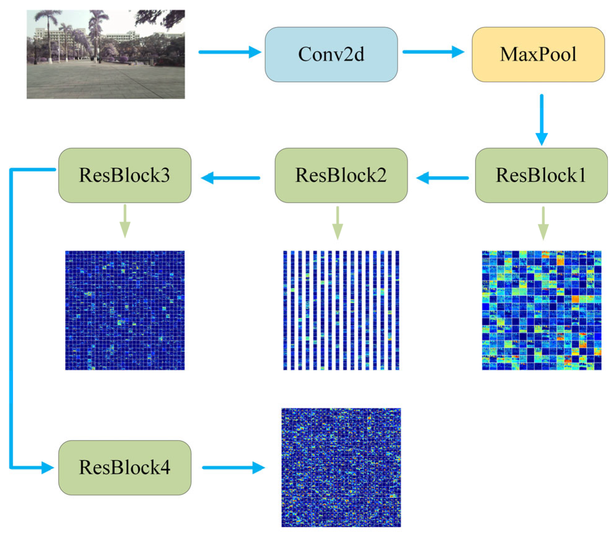
3.1. Visual Relocalization in Autonomous Vehicles

1.

Construction of the Map Scene Database;

The map data are collected using the stereo visual camera and RTK system mounted on the autonomous vehicle. The MonSter [37] model calculates the disparity in the images. From this, depth information is derived using disparity-depth conversion. The pose information, RTK coordinates, and depth data for each image are linked to its image ID. Each image, along with its pose, RTK coordinates, and depth data, is stored in the database. This completes the map scene database construction.

2.

Neural Network-Based Image Retrieval System;

This section presents a neural network-based image retrieval system. Neural networks are better at feature encoding than traditional content-based methods. They can directly extract high-dimensional features from images. We use the ResNet-50 model for feature extraction. The model’s shortcut connections help improve communication between feature vectors in different high-dimensional spaces. This design increases image classification accuracy without adding many parameters.

The ResNet-50 model comprises 50 layers and is organized into four stages. Stage 1 contains three residual units, Stage 2 has four, Stage 3 includes six, and Stage 4 consists of three residual units. Each residual unit comprises three convolutional layers. The network also includes an initial convolutional layer, followed by a pooling layer and a fully connected layer at the end. To extract high-dimensional global image features for practical applications, the original architecture was modified in this study by removing the final pooling and fully connected layers. Figure 2 presents the visualizations of the output features from each residual block. Taking into account both the representational power and dimensionality of the features, the output of the fourth residual block is selected as the global descriptor. This descriptor is subsequently employed for image similarity measurement and retrieval-based matching tasks.

After feature extraction of the images in the database using ResNet-50, a set of feature vectors V_base is obtained and stored as the feature descriptor database. For a query input image I_q, its feature vector V_Iq is extracted using ResNet-50. The similarity between V_Iq and all feature vectors in V_base is then computed. The image with the highest similarity is selected as the retrieved image I_k, and its corresponding feature descriptor vector is V_Ik. The similarity is calculated as the cosine of the angle between the vectors in the feature space, with the formula given in Equation (1):

$$Similarity(V_{Iq},V_{Ik})={\displaystyle \frac{<V_{Iq}•V_{Ik}>}{\left|V_{Iq}\right|\left|V_{Ik}\right|}},$$

(1)

3.

Depth Estimate;

Due to the unique design of stereo cameras, depth estimation can be achieved by comparing the images captured by the left and right cameras to calculate their disparity. Based on the principle of triangulation, the depth of each image point can be estimated.

The stereo camera model is illustrated in Figure 3. In this model, $O_L$ and $O_R$ represent the optical centers of the left and right cameras, respectively. A 3D point $p$ is projected onto the left and right image planes as $P_L$ and $P_R$. The baseline $b$ denotes the distance between the optical centers, and $f$ is the focal length. $u_L$ and $u_R$ are the horizontal coordinates of $P_L$ and $P_R$. Typically, the two image planes are coplanar and horizontally aligned. Based on triangulation, the depth $z$ can be computed as:

$$\left({\displaystyle \frac{z-f}{z}}\right)=\left({\displaystyle \frac{b-u_L+u_R}{b}}\right),$$

(2)

After organizing the equations, we have:

$$z={\displaystyle \frac{fb}{d}}, d=u_L-u_R,$$

(3)

Here, $d$ denotes the disparity, the horizontal coordinate difference between corresponding points in the left and right images. Although the depth formula is mathematically simple, its practical computation is often challenging due to the difficulty in accurately locating the corresponding points between the two images.

MonSter introduces a dual-branch depth estimation framework that integrates monocular depth estimation and stereo matching based on 3D point clouds. It is designed to handle complex and structured scenes with improved stability and accuracy. The framework consists of two main components: one branch for monocular depth estimation and another for stereo matching based on 3D point clouds. The monocular branch estimates depth using high-resolution image features and semantic information, while the stereo branch compensates for the scale drift commonly found in traditional monocular methods by incorporating geometric constraints and image correspondences.

MonSter effectively fuses geometric and photometric information through structural guidance and dual-branch optimization, establishing a coarse-to-fine depth estimation pipeline. This method addresses issues such as depth ambiguity, low-texture regions, and occlusion, which frequently occur in long-range scenes or when key targets are missing, thereby significantly enhancing the robustness of stereo matching. By improving accuracy, stability, and reliability, MonSter offers an effective solution for depth sensing.

To compute disparity from stereo image pairs, this study utilizes the MonSter network. Given that the stereo camera is pre-calibrated, the disparity values can be accurately converted into depth information using the calibration parameters and corresponding equations. The resulting depth data are then stored in a database to enable efficient retrieval and utilization during subsequent 3D coordinate reconstruction.

4.

Feature Matching;

After obtaining the most similar matching image I_k to the input image I_q, the next step is to establish the correspondence between the image pair to perform pose estimation. Traditional methods generally involve extracting local feature points from both the input and matching images to identify their correspondences. The relative pose is subsequently computed using epipolar geometry. Finally, the global pose of the matching image in the world coordinate system is used to infer the pose of the input image within the same global coordinate system.

However, the relative pose calculated using traditional methods often exhibits substantial deviations. To address this issue, we adopt a deep learning-based feature matching approach. Specifically, for the image pair I_q and I_k, we perform feature matching using the integrated feature matching model framework proposed in this paper. This approach enhances both the accuracy of feature matching and the precision of pose estimation.

5.

Pose Estimation;

For the visual relocalization task, the query image I_q is matched with candidate images I_k, retrieved by a neural network, through feature point matching. By performing feature matching and filtering, a stable set of correspondences $P_q^f$ and $P_k^f$ is obtained. For each retrieved image I_k, which is associated with a depth map $I_{k-depth}$ and a known camera pose $T_{wc}^k$ in the world coordinate system, the matched points $P_k^f$ can be transformed into their corresponding $P_w$ 3D world coordinates using the pinhole camera model. The transformation is defined as:

$$P_w=z_k{T}_{wc}^k{K}^{-1}{P}_k^f,$$

(4)

where $z_k$ denotes the depth value of the matched pixel $P_k^f$ in the depth map, and $K$ is the intrinsic parameter matrix of the camera used to capture the image.

From the obtained 2D–3D feature correspondences, valid correspondences with depth values are first selected from I_k, yielding a candidate set of $N^{depth}$ points for subsequent pose estimation. Then, $N^{select}$ points are randomly sampled from this set for nonlinear optimization, while the remaining points are used in the PnP algorithm to compute the initial camera pose, as shown in Figure 4, providing an initial estimate for Levenberg–Marquardt (L-M) optimization. During this process, the following objective function is minimized to reduce the reprojection error:

$$T^{*}=\underset{T}{\arg \min }{\displaystyle \frac{1}{2}}{\displaystyle \sum _{i=1}^{N^{select}}{‖P_q^f(i)-\frac{1}{z_i}KT{P}_w(i)‖}_2^2},$$

(5)

where $z_i$ is the depth of the $i$-th 3D landmark in the camera coordinate system, and $T$ denotes the camera pose to be optimized.

Among nonlinear least squares methods for pose estimation, the Gauss–Newton algorithm is one of the most commonly used approaches. However, it suffers from several practical limitations. The approximate Hessian matrix constructed by the method can become singular or ill-conditioned in certain cases, making the resulting linear system difficult to solve and reducing the stability and convergence of the algorithm. Moreover, since the Gauss–Newton method is derived from a second-order Taylor expansion, its approximation is only accurate within a small neighborhood. If the computed step size is large, the approximation error may increase significantly, potentially causing the optimization to diverge. To address these issues, the Levenberg–Marquardt (L-M) algorithm introduces regularization strategies that enhance both the stability and convergence of the optimization process.

Following nonlinear optimization, the selected 3D landmark points used for error minimization are projected onto the image plane to obtain their corresponding 2D projections. These projected points are then compared with the actual image feature points $P_q^f$ to calculate the reprojection error. If the reprojection error for all matched points is below a predefined threshold, the pose estimation is deemed to have converged. Consequently, the optimization process terminates, and the final camera pose is reported.

3.2. Integrated Matching Model Framework

In the proposed framework, we have obtained an image pair consisting of the input image I_q and the matching image I_k, and accurate correspondences between these images are essential for pose estimation. Correctly establishing these correspondences can significantly enhance the accuracy of visual localization. However, modern deep learning-based feature matching models often require considerable computational resources and extensive training time, which can be a limiting factor in real-time applications. To address this challenge, we have developed a feature matching algorithm based on an integrated model that strikes a balance between computational efficiency and matching accuracy.

Figure 5 presents the feature matching algorithm framework. This algorithm combines two methods: the detector-based “Superpoint+LightGlue [38]” and the detector-free LoFTR. The “Superpoint+LightGlue” method detects local feature points and matches their descriptors to extract key features. It establishes precise correspondences between images. LoFTR, on the other hand, uses a deep learning model to learn global image features. This allows for more accurate dense matching, even with image deformations or changes in viewpoint. By combining both methods, we achieve more accurate correspondences across different scenes and environments. This enhances the accuracy and robustness of visual localization.

SuperGlue employs multilayer perceptrons (MLPs) to encode keypoint positions. However, this encoding method may result in the loss of positional information during inter-layer propagation, thereby reducing matching accuracy. Additionally, the algorithm is computationally intensive and memory-demanding. To overcome these limitations, LightGlue has been proposed as a more efficient feature matching method that significantly improves training complexity, computational efficiency, and resource utilization.

We introduced a multi-scale transformation input method to improve image matching performance. The algorithm uses the original image resolution and applies transformations at different scales, such as scaling and blurring. This helps the algorithm capture finer details, especially in scenes with significant variations in scale or viewpoint. As a result, the matching process becomes more accurate and robust. By using multi-scale inputs, the algorithm matches features at various levels. This gives a more complete understanding of the image content and enhances the precision of the final pose estimation.

Initially, multi-scale and multi-orientation transformations are applied by resizing both the input and reference images to three resolutions—400, 800, and 1600 pixels—and rotating them at various angles to generate diverse image pairs. In the first stage of feature matching, “SuperPoint+LightGlue” and LoFTR algorithms are employed to obtain an initial set of correspondences. The resulting feature matches are then analyzed using the DBSCAN clustering algorithm with adaptive parameter estimation to identify densely matched regions, which are subsequently extracted and defined as co-visibility regions.

To further improve matching accuracy, these co-visibility regions are designated as Building Boxes and subjected to an additional refinement step. Within each Building Box, a second round of multi-scale feature matching is conducted using both LoFTR and “SuperPoint+LightGlue”, yielding more precise matching results.

Finally, correspondences from both matching stages are concatenated to form a comprehensive set. To eliminate outliers and retain only reliable matches, a geometry-consistency-based inlier selection method is employed for inlier filtering. This multi-stage, multi-scale matching pipeline enables the acquisition of highly accurate and dense image correspondences, thereby providing robust input for subsequent pose estimation.

The proposed method increases the number of matched point pairs by applying multi-scale transformations, including image scaling and rotation, during feature matching. However, these transformations can introduce errors that result in a high number of incorrect matches in the initial matching stage. To address this issue, we apply the DBSCAN algorithm for preliminary outlier removal. Despite its effectiveness, DBSCAN is highly sensitive to parameter selection, and its clustering performance largely depends on these parameters. In complex feature matching scenarios—characterized by noise, transformation model complexity, and feature similarity—manually selecting appropriate parameters is challenging and often impractical. To address these challenges, the improved DBSCAN algorithm known as HDBSCAN is utilized. HDBSCAN is a density-based hierarchical clustering method that analyzes cluster structures across multiple density levels, enabling automatic determination of the number of clusters while effectively identifying noise points. Unlike traditional DBSCAN, HDBSCAN measures the connectivity between sample points using the mutual reachability distance. The core of the method involves computing the mutual reachability distance between any two points as defined by Equation (6).

$$d_{\mathrm{mreach}}(a,b)=\max ({\mathrm{core}}_k(a),{\mathrm{core}}_k(b),d(a,b)),$$

(6)

Here, $d(a,b)$ denotes the Euclidean distance, while ${\mathrm{core}}_k(x)$ represents the distance from point $x$ to its $k$-th nearest neighbor, which serves as a measure of the point’s local density.

As shown in Figure 6, the mutual reachability distance from the red point to the blue point corresponds directly to the distance between them, since this distance exceeds both core distances.

The algorithm proceeds by modeling the distance structure among samples through the construction of a minimum spanning tree (MST). A graph is formed by connecting each point to its nearest neighbors within its reachable range, with edge weights defined by the mutual reachability distance described previously. Prim’s algorithm is then applied to generate the MST, preserving the most critical density-based connectivity among data points. Edges in the MST are subsequently removed in descending order of mutual reachability distance to form a hierarchical cluster structure. Initially, each point constitutes an individual cluster, and clusters are iteratively merged based on proximity, producing a hierarchical clustering tree.

Following the construction of the hierarchical clustering tree, a condensation process compresses the large tree into multiple smaller sub-clusters. HDBSCAN introduces a parameter, minimum cluster size, to govern the splitting of the hierarchical tree. The condensation begins at the root node, where the entire dataset is treated as a single cluster. For each cluster represented by a node, the algorithm first evaluates its sample size. Clusters with fewer samples than the minimum cluster size are considered invalid and are either discarded or labeled as noise. Clusters meeting the minimum size threshold are further examined for their sub-cluster structures. Through this recursive exploration and filtering, the original hierarchical clustering tree is reduced to a set of appropriately sized, well-defined subtrees. Each subtree’s root node represents a stable cluster that satisfies the parameter criteria.

HDBSCAN enhances the algorithm’s adaptability by eliminating the need for users to predefine the number of clusters. Instead, it automatically determines the clustering structure based on the data’s density features and cluster stability. Noise points are removed during the condensation process, which improves the robustness of the clustering results. Moreover, HDBSCAN introduces cluster stability as a metric for evaluating clustering quality. The core idea is that the longer a sample remains within a cluster, the higher the confidence in its membership. Cluster stability is quantified by Equation (7).

$$S_{\mathrm{cluster}}={\displaystyle \sum _{p\in \mathrm{cluster}}({\lambda }_{\mathrm{p}}-{\lambda }_{\mathrm{birth}})},$$

(7)

where $\lambda$ denotes the reciprocal of the mutual reachability distance between data points; ${\lambda }_{\mathrm{birth}}$ represents the density threshold at which the cluster initially splits; and ${\lambda }_{\mathrm{p}}$ corresponds to the density threshold at which a sample exits the cluster.

The formula quantifies the cumulative “survival” time of each sample within a cluster, thereby serving as an indirect measure of the cluster’s stability. Greater stability indicates that the cluster consistently maintains its characteristics across multiple scales, rendering it more representative and interpretable.

After configuring all experimental parameters, clustering results were employed to eliminate outliers from the initial set of matched points, producing a refined matched point set denoted as Stage1. These clusters are typically concentrated within corresponding regions of the two images, which are defined here as co-visible areas. Such co-visible regions generally contain abundant local feature information. To generate additional matched point pairs, the overall co-visible region was extracted via bounding box cropping and treated as an independent image. This region was then reprocessed through the feature matching module for a second matching iteration, yielding an additional matched point set, Stage2. Subsequently, Stage2 was concatenated with Stage1 to form the combined set StageAll. Given that this combined set may still include mismatches and duplicate pairs, further refinement is necessary to obtain a higher-quality final matching set.

To effectively remove mismatched pairs from the coarse matching set, robust inlier selection algorithms are commonly employed. This study utilizes a geometry-consistency-based inlier selection method to filter inliers satisfying geometric constraints from the matched points, thereby enhancing the accuracy and robustness of subsequent relocalization modules. The core principle involves constructing a cost function based on epipolar geometry constraints, integrating an error model with maximum consensus search, and iteratively optimizing the fundamental matrix model that best fits the distribution of point pairs to identify the inlier set.

The fundamental matrix describes the geometric relationship between two different viewpoints and encodes the epipolar constraint between image pairs resulting from the projection of a 3D point onto two image planes. Suppose a 3D point $P$ projects onto a pair of corresponding points $\left(p_1,p_2\right)$ in two images, where $p_1$ lies in image $I_1$ and $p_2$ lies in image $I_2$. These points must satisfy the epipolar geometric relationship defined by the fundamental matrix. As shown in Figure 7, satisfying the epipolar constraint. This condition can be expressed as:

$${p_2}^{T}F{p}_1=0,$$

(8)

where $F$ is the fundamental matrix, which has rank 2.

Due to the inevitable presence of mismatches in the StageAll set, directly estimating the fundamental matrix using all point pairs is highly vulnerable to outliers, which can lead to inaccurate model estimation. To enhance the robustness of the fitting process, this study employs a robust estimation method based on the principle of consensus sampling. Specifically, the improved RANSAC variant MAGSAC++ [39] is adopted as the model estimation algorithm. Built upon the traditional RANSAC framework, MAGSAC++ introduces multiple enhancements in statistical modeling and scoring mechanisms, significantly improving its resilience to incorrect correspondences.

The estimation begins by randomly selecting a minimal sample set—typically eight point pairs—from the set of matches. The eight-point algorithm is then applied to estimate a candidate fundamental matrix. Once the model is fitted, the algorithm evaluates the consistency between all point pairs and the estimated model by computing the geometric error for each correspondence. The Sampson distance, a commonly used error metric, is employed due to its close approximation of the epipolar constraint residual, along with its strong geometric interpretability and numerical stability. The computation is provided in Equation (9)

$$d_{\mathrm{Sampson}}(p_1,p_2,F)={\displaystyle \frac{{({p_2}^{\mathrm{T}}F{p}_1)}^2}{{(F{p}_1)}_1^2+{(F{p}_1)}_2^2+{(F^{\mathrm{T}}{p}_2)}_1^2+{(F^{\mathrm{T}}{p}_2)}_2^2}},$$

(9)

Unlike traditional RANSAC, MAGSAC++ does not distinguish inliers from outliers using a fixed threshold. Instead, it maps each residual error to a continuous score based on a marginalized likelihood function. This approach, rooted in the probabilistic framework of maximum likelihood estimation, employs a weighted loss function to marginalize the residuals of all point correspondences. The continuous scoring mechanism avoids the instability caused by threshold selection and provides a more accurate reflection of each point pair’s compatibility with the model.

After each sampling iteration, MAGSAC++ calculates the model score and selects the model with the highest score as the optimal solution. Once the best model is determined, it re-evaluates the geometric error for all matched points and uses a probabilistic scoring function to assess the confidence of each point being an inlier. This process significantly improves model estimation robustness under high noise and high outlier ratio conditions.

By incorporating both geometric error and the statistical distribution and uncertainty of residuals, MAGSAC++ exhibits superior inlier selection performance in practical visual matching tasks.

4. Experiment

4.1. Experimental Setup

The implementation is developed using Python 3.8. The system configurations are as follows: the central processing unit (CPU) is an Intel Core i7-13700KF with 24 cores running at 3.40 GHz, the system memory is 32 GB, the graphics processing unit (GPU) is an NVIDIA GeForce RTX 4080 with 16 GB of VRAM, and the operating system is Ubuntu 20.04 LTS. We employed several software libraries in our implementation, including OpenCV, PyTorch, NumPy, and Kornia.

4.2. Evaluation of Feature Matching Accuracy

Feature matching is a fundamental step in many computer vision tasks. To evaluate the robustness and effectiveness of the proposed algorithm under challenging conditions—such as significant variations in illumination and viewpoint—this study designs a feature matching accuracy evaluation experiment and systematically analyzes and verifies its performance.

4.2.1. Datasets

The HPatches [40] dataset was used for evaluation. It comprises 108 image sequences, including 52 sequences with viewpoint variations and 56 sequences with illumination changes. Each sequence contains six images captured under different viewpoints or lighting conditions, along with the corresponding essential matrices. An example of a sequence exhibiting viewpoint variation is shown in the Figure 8.

4.2.2. Metrics

In this experiment, the mean matching accuracy (MMA) across all image pairs is adopted as the evaluation metric. A predicted correspondence is considered correct if its reprojection error is below a specified threshold, ranging from 1 to 10 pixels; otherwise, it is regarded as incorrect.

4.2.3. Results

This experiment utilizes the Matching Mean Accuracy (MMA) metric to quantitatively evaluate the feature matching performance of the proposed method under various challenging conditions, within an error threshold range of 1–10 pixels. As illustrated in Figure 5, the proposed approach consistently outperforms mainstream state-of-the-art methods across all test scenarios, including comparisons with LoFTR and SuperPoint+LightGlue.

In illumination variation scenes, our method achieves the highest matching accuracy at all pixel thresholds, demonstrating strong robustness to lighting changes. Notably, under smaller thresholds (1–3 pixels), it significantly outperforms conventional methods, indicating superior performance in fine-grained feature matching tasks. In viewpoint variation scenarios, the method also exhibits exceptional adaptability, effectively handling geometric transformations caused by perspective changes, with matching accuracy markedly surpassing that of baseline approaches.

Comprehensive evaluation results show that the proposed algorithm maintains top performance across the full range of error thresholds, highlighting its overall robustness in dealing with complex environmental changes. Particularly under low-error conditions, it demonstrates higher matching accuracy than existing methods, further underscoring its practical applicability and potential for real-world deployment.

Overall, the proposed matching framework outperforms existing algorithms in multiple challenging scenarios in terms of accuracy and stability. By effectively combining the strengths of detector-free and detector-based methods, it leverages their complementary advantages in feature extraction and matching. Additionally, the introduction of a coarse-to-fine inlier filtering mechanism enhances both the accuracy and robustness of the matching results, significantly improving the algorithm’s generalization capability across diverse environments.

4.3. Homography Estimation Experiment

Achieving high-precision feature matching does not necessarily ensure the accurate recovery of the geometric relationship (e.g., relative pose) between two images. In addition to matching accuracy, the number of feature points and their spatial distribution across the image are also critical factors. To further assess the applicability of the proposed method for geometric estimation tasks, a homography estimation experiment was conducted.

4.3.1. Datasets

In the homography estimation experiment, the dataset used was the same as that employed in the feature matching accuracy experiment, specifically HPatches.

4.3.2. Metrics

In this experiment, the mean matching accuracy (MMA) across all image pairs is adopted as the evaluation metric. A predicted correspondence is considered correct if its reprojection error is below a specified threshold, ranging from 1 to 10 pixels; otherwise, it is regarded as incorrect.

This paper employs the corner accuracy metric to evaluate the performance of the algorithm. The metric is based on the reprojection error of four corner points in an image, and the proportion of images with an average reprojection error below 1, 3, or 5 pixels is computed. Specifically, the proposed algorithm is first applied for feature matching, and the predicted homography matrix between two matched images is computed using functions from OpenCV. Using the predicted homography matrix $\tilde{H}$ and the ground truth homography matrix $H$, the four corner points of the first image are projected onto the second image, and the average reprojection error $\epsilon$ is calculated. Finally, the proportion of images with reprojection errors below a predefined threshold is computed to assess the algorithm’s matching accuracy.

4.3.3. Results of the Homography Estimation Experiment

As shown in

Table 1. Results of the Homography Estimation Experiment. Bold values represent the best results among all methods.

Method	Overall	Illumination	Viewpoint
	Accuracy ($\mathit{\epsilon }$ < 1/3/5 Pixel)
D2-Net [34]	0.38/0.71/0.82	0.66/0.95/0.98	0.12/0.49/0.67
R2D2 [41]	0.47/0.77/0.82	0.63/0.93/0.98	0.32/0.64/0.70
SP [32]+LG [38]	0.39/0.85/0.90	0.52/0.96/0.98	0.28/0.75/0.84
Sparse-NCNet [42]	0.36/0.65/0.76	0.62/0.92/0.97	0.13/0.40/0.58
Patch2Pix [43]	0.50/0.79/0.87	0.71/0.95/0.98	0.30/0.64/0.76
LoFTR [36]	0.55/0.81/0.86	0.74/0.95/0.98	0.38/0.69/0.76
MatchFormer [44]	0.55/0.81/0.87	0.75/0.95/0.98	0.37/0.68/0.78
OURS	0.55/0.83/0.88	0.76/0.96/0.98	0.33/0.69/0.78

, The proposed matching algorithm, which fuses detector-based and detector-free approaches, demonstrates outstanding performance in homography estimation tasks. Under certain evaluation metrics, it achieves the highest accuracy. Specifically, the corner accuracy at 1, 3, and 5-pixel error thresholds reaches 0.55, 0.83, and 0.88, respectively, which is comparable to that of the detector-based SuperPoint+LightGlue and the detector-free LoFTR. Notably, it achieves the best performance at the 1-pixel threshold.

In terms of illumination robustness, the method achieves accuracy rates of 0.76, 0.96, and 0.98 under the same thresholds, outperforming all other evaluated algorithms. This advantage stems from the effective complementarity between stable local features provided by the detector and the global matching strategy of the detector-free component. Moreover, the method exhibits strong robustness to viewpoint variations, further confirming its adaptability to scenarios involving significant geometric transformations.

4.4. Pose Estimation Experiments in Indoor and Outdoor Environments

Pose estimation is a fundamental research area in mobile robotics. However, achieving high-precision pose estimation in complex environments remains a significant challenge due to factors such as motion blur and repetitive textures. This challenge becomes even more pronounced in outdoor settings, where the intricate 3D structures and significant variations in viewpoint and lighting conditions further complicate the estimation process. To further assess the effectiveness of the proposed algorithm, pose estimation experiments were conducted on widely used indoor and outdoor public datasets, systematically evaluating its robustness and accuracy across various scenarios.

4.4.1. Datasets

For indoor pose estimation, the ScanNet dataset was used for validation. This dataset consists of 1613 monocular images, each accompanied by corresponding pose and depth maps. It presents significant challenges for matching algorithms, including issues with wide baseline matching and textureless regions. For outdoor pose estimation experiments, the MegaDepth dataset was employed. This dataset contains 196 outdoor scenes and over one million internet-sourced images, which include a wide range of viewpoint changes and repetitive textures. The images, taken from tourist photographs, exhibit significant variations in lighting and viewpoint, providing valuable experimental data for training robust pose estimation models.

4.4.2. Metrics

This experiment adopts the widely used evaluation metric introduced by the SuperGlue [35] method, which assesses algorithm performance by calculating the area under the cumulative error distribution curve at various thresholds (Area Under Curve, AUC). Pose error is defined as the maximum of the translation vector and the angular error of the rotation vector between the predicted and true poses. Specifically, at thresholds of 5°, 10°, and 20°, the AUC values corresponding to each threshold are computed using the Receiver Operating Characteristic (ROC) curve, providing a comprehensive evaluation of the proposed algorithm’s performance.

4.4.3. Experimental Results on Scannet and MegaDepth

To validate the effectiveness of the proposed integrated matching model, we improved an existing open-source algorithm and conducted comparative tests between the enhanced matching method and other feature matching algorithms on the MegaDepth and ScanNet datasets.

For the MegaDepth dataset, we selected 1500 image pairs for evaluation and established three thresholds for pose estimation error: 5°, 10°, and 20°. To solve the camera pose estimation problem, we employed the RANSAC algorithm to compute the fundamental matrix from the predicted matches. The evaluation results of the improved matching algorithm, compared to other open-source algorithms, are presented in

Table 2. Pose Estimation Results on the MegaDepth Dataset. Bold values represent the best results among all methods.

Category	Method	Pose Estimation AUC%
		AUC@5°	AUC@10°	AUC@20°
Sparse	SP [32] + NN	31.7	46.8	60.1
	SP [32] + SG [35]	49.7	67.1	80.6
	SP [32] + LG [38]	49.9	67.0	80.1
Semi-Dense	DRC-Net [45]	27.0	42.9	58.3
	LoFTR [36]	52.8	69.2	81.2
	QuadTree [46]	54.6	70.5	82.2
	MatchFormer [44]	53.3	69.7	81.8
	TopicFM [47]	54.1	70.1	81.6
	OURS	55.6	70.6	82.1

. The evaluation metric used is the Area Under the ROC Curve (AUC) at various thresholds.

For the ScanNet dataset, we selected 1500 image pairs for testing, using three pose estimation error thresholds: 5°, 10°, and 20°. To recover the camera pose, we employed the RANSAC algorithm to compute the fundamental matrix from the predicted matches. The evaluation results of the improved algorithm, compared with other matching algorithms, are presented in

Table 3. Pose Estimation Results on the ScanNet Dataset. Bold values represent the best results among all methods.

Category	Method	Pose Estimation AUC%
		AUC@5°	AUC@10°	AUC@20°
Sparse	ORB [31] + GMS [48]	5.2	13.7	25.4
	SP [32] + NN	7.5	18.6	32.1
	SP [32] + SG [35]	16.2	32.8	49.7
	SP [32] + LG [38]	14.8	30.8	47.5
Semi-Dense	DRC-Net [45]	7.7	17.9	30.5
	LoFTR [36]	16.9	33.6	50.6
	MatchFormer [44]	15.8	32.0	48.0
	TopicFM [47]	17.3	35.5	50.9
	OURS	19.1	36.4	52.6

.

The results presented in Table 1 and Table 2 show that, after integrating the matching framework with the open-source algorithm model, the improved algorithm consistently achieves significantly higher AUC values across all thresholds compared to other methods. This integrated framework not only improves accuracy on the MegaDepth dataset but also outperforms other algorithms on the ScanNet dataset. The evaluation metrics generally exceed the performance of individual models, demonstrating that the proposed matching method effectively enhances matching accuracy.

These findings indicate that, without requiring additional training on the dataset, the proposed algorithm framework successfully improves matching accuracy while reducing computational resource consumption. Validation on public datasets further confirms the effectiveness and feasibility of the proposed framework.

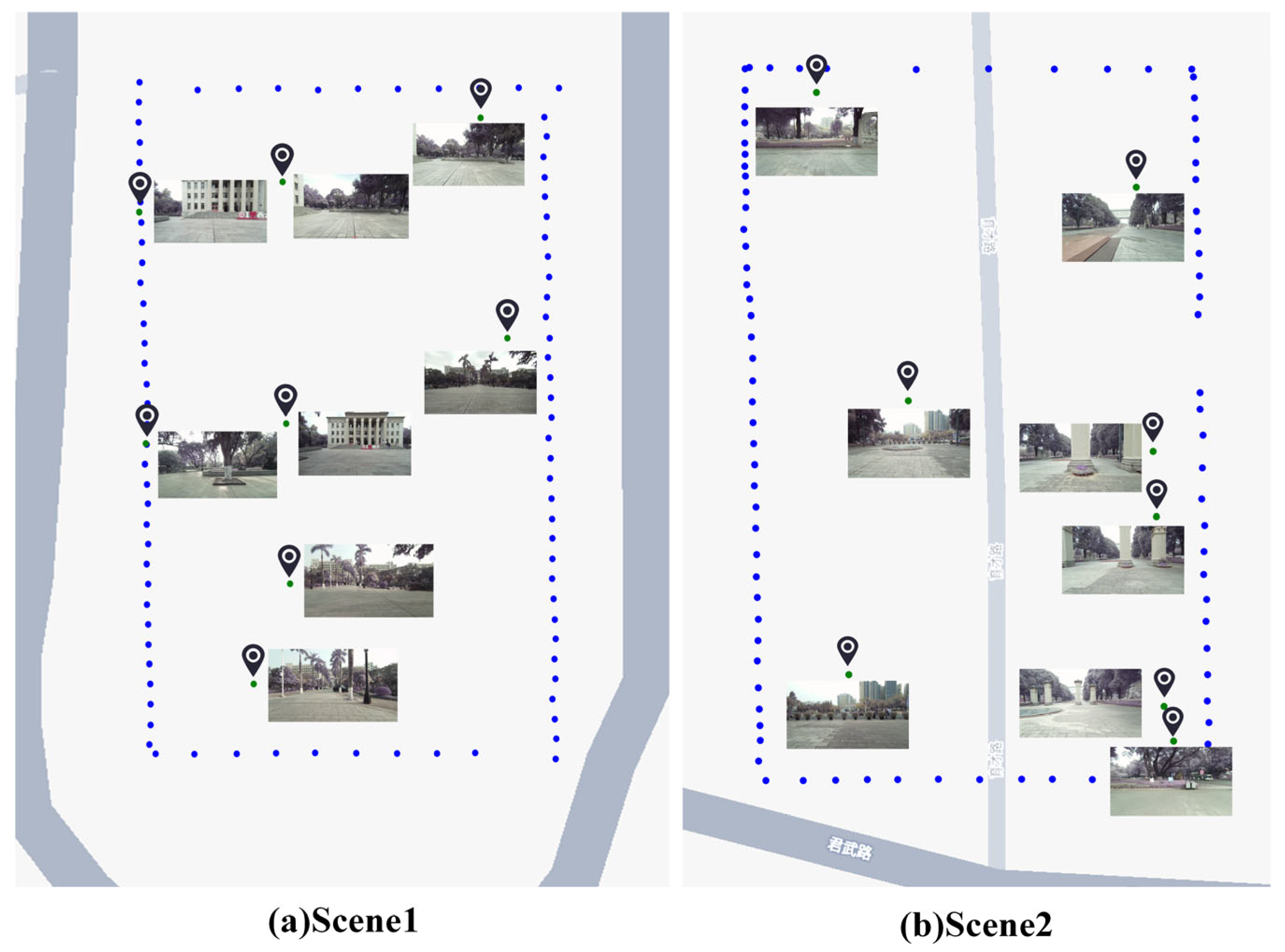
4.5. Experiments in Outdoor Real-World Scenarios

To assess the practical applicability of the proposed method, we constructed a field dataset using a self-developed autonomous vehicle equipped with a camera and RTK system. Initially, the vehicle was remotely controlled to capture images of the surrounding environment. These images were timestamped and matched with the corresponding RTK coordinate data, and then stored in the map database. Subsequently, depth information for each image was obtained using a stereo camera and depth estimation module, and the depth data were saved along with the images in the database. Following the vehicle’s reboot, we validated the relocalization functionality by capturing an image from any location within the scene to serve as the query image.

The evaluation metric for the field scenario dataset is the Euclidean distance error between the RTK coordinates and the predicted coordinates generated by the proposed method. This dataset was constructed in a real-world environment and was not used for training the model, thereby providing a robust means of validating the practical applicability and generalization of the method. Validation using this dataset enables an assessment of the method’s performance in real-world conditions, further confirming its robustness and accuracy in actual environments.

4.5.1. Preparation Phase

In the preparation phase, the autonomous vehicle traversed the site, capturing RGB images with a stereo camera. Concurrently, the RTK system recorded the vehicle’s real-time coordinates to ensure precise location data. The stereo camera images were then processed by the depth estimation module to generate depth information for each frame. The primary objective of this phase was to gather both visual data of the site and accurate location information, which will serve as the foundation for subsequent map construction and localization tasks.

ResNet-50 was employed as the feature extraction network to derive features from the left-eye images. These extracted features, along with the RTK coordinates, depth information, and original images, were stored in the database. Serving as the core of the map, this database stores both the visual features and associated geometric data for various locations within the site. This process ensures the database is complete and accurate. It provides a reliable reference for image matching and localization during the testing phase.

4.5.2. Preparation Phase

In the testing phase, the autonomous vehicle system is activated. It captures images of the test site using a stereo camera. The system processes the left-eye image to extract feature descriptors. These descriptors are then sent to the similarity computation module. In this module, the descriptors are compared to the images in the map database. The image with the highest similarity is chosen as the matching image.

Upon identifying a matching image, the input and matching images are paired and fed into the feature matching network. The depth information of the matching image from the database is then compared, establishing a 2D–3D correspondence between the input and matching images. This correspondence enables the system to estimate the position and orientation of the input image in 3D space. The pose estimation algorithms are subsequently applied to optimize reprojection errors, resulting in more accurate pose estimation.

To assess the effectiveness of the proposed relocalization algorithm, this study emphasizes its generalization ability in unknown environments. The algorithm’s performance is evaluated across various outdoor conditions by collecting a real-world dataset.

Figure 9 illustrates the data collection details and trajectory of the autonomous vehicle across two distinct outdoor scenes. The blue dots indicate the location coordinates recorded by the vehicle as it navigated the site. These points represent the vehicle’s route during the map database construction phase. In the outdoor scenario, we instructed the autonomous vehicle to complete a lap around the site, capturing images at locations marked by the blue points in Figure 5. After constructing the map database, we selected eight distinct positions for testing in both Scene 1 and Scene 2. The images and corresponding locations are represented by the green points in Figure 10.

Figure 10 depicts the data collection process during the testing of the autonomous vehicle in two outdoor scenarios. The green points and corresponding images represent the location coordinates and image data captured by the vehicle after the map database was constructed. These data are collected to enable the relocalization function, which allows the vehicle to determine its position within the map during subsequent processes. Using the collected data, the proposed relocalization method is applied to evaluate the vehicle’s relocalization performance. The predicted map coordinates for each test point are compared with the original coordinates, as shown in Figure 11. The experimental results and errors are summarized in

Table 4. Relocalization Function Test Results in Scene 1.

Actual Coordinates		Relocalization		Metrics
Input Images	Measured Coordinates (N, E)	Matching Image	Predicted Coordinates (N, E)	Coordinate Error (▲N, ▲E)	Translation Error (m)
Test1	(2,526,947.321, 529,196.851)	Map03	(2,526,947.469, 529,196.997)	(−0.148, −0.146)	0.208
Test2	(2,526,950.403, 529,197.401)	Map09	(2,526,950.003, 529,197.494)	(0.400, −0.093)	0.411
Test3	(2,526,955.328, 529,197.345)	Map21	(2,526,954.959, 529,197.237)	(0.369, 0.108)	0.384
Test4	(2,526,962.757, 529,197.288)	Map27	(2,526,963.033, 529,197.179)	(−0.276, 0.109)	0.297
Test5	(2,526,964.728, 529,200.288)	Map40	(2,526,964.317, 529,200.125)	(0.411, 0.163)	0.442
Test6	(2,526,961.826, 529,195.117)	Map25	(2,526,962.651, 529,194.450)	(−0.825, 0.667)	1.061
Test7	(2,526,957.945, 529,200.695)	Map56	(2,526,958.586, 529,200.175)	(−0.641, 0.520)	0.825
Test8	(2,526,954.711, 529,195.219)	Map14	(2,526,955.301, 529,195.683)	(−0.590, −0.464)	0.751

and

Table 5. Relocalization Function Test Results in Scene 2.

Actual Coordinates		Relocalization		Metrics
Input Images	Measured Coordinates (N, E)	Matching Image	Predicted Coordinates (N, E)	Coordinate Error (▲N, ▲E)	Translation Error (m)
Test1	(2,526,492.846, 529,213.087)	Map87	(2,526,492.263, 529,213.078)	(−0.582, −0.009)	0.583
Test2	(2,526,494.824, 529,212.805)	Map05	(2,526,494.824, 529,213.010)	(0.000, 0.205)	0.205
Test3	(2,526,505.666, 529,212.576)	Map13	(2,526,506.105, 529,212.897)	(0.439, 0.321)	0.544
Test4	(2,526,509.387, 529,212.480)	Map15	(2,526,509.351, 529,212.906)	(−0.036, 0.426)	0.428
Test5	(2,526,524.473, 529,211.980)	Map25	(2,526,524.934, 529,211.925)	(0.461, −0.055)	0.464
Test6	(2,526,529.884, 529,202.476)	Map37	(2,526,530.136, 529,202.393)	(0.252, −0.083)	0.265
Test7	(2,526,512.270, 529,205.204)	Map61	(2,526,512.405, 529,204.933)	(0.135, −0.271)	0.303
Test8	(2,526,496.651, 529,203.441)	Map72	(2,526,496.683, 529,203.215)	(0.032, −0.226)	0.228

.

Table 4 presents the localization performance of the proposed method in Scene 1. A systematic analysis of eight test data (Test1–Test8) shows that the method achieves precise vehicle localization, with the error between predicted and actual coordinates remaining low. Specifically, the average translation error in the planar coordinate system is 0.491 m. Test1 demonstrates the best performance, with an error of only 0.208 m, while Test6 exhibits a relatively larger error of 1.061 m. Nevertheless, error analysis reveals that, in most test cases, the method can maintain the error within a 0.5 m range. The experimental results fully validate the effectiveness and reliability of the proposed method for autonomous vehicle map localization.

As shown in Table 5, the proposed localization method exhibits excellent performance in the Scene 2 testing. To assess the algorithm’s applicability across different scenarios, we collected eight test datasets (Test1–Test8) in Scene 2 and conducted quantitative analysis. The results demonstrate that the proposed method maintains stable localization accuracy in various environments. Specifically, the average translation error in Scene 2 is 0.377 m, with Test2 showing the best performance, yielding an error of only 0.205 m. The largest error occurred in Test3, with a value of 0.544 m. In all test cases, the errors were kept within 0.6 m, with minimal fluctuations, indicating that the proposed method can effectively achieve vehicle localization in diverse environments.

Figure 11 presents the map displaying the coordinates predicted by the relocalization algorithm across different scenes. The red dots represent the predicted position coordinates, while the green dots indicate the true coordinates obtained through RTK measurements. The experimental results from two real-world scenarios demonstrate that the proposed relocalization method achieves high accuracy in both outdoor environments, effectively determining the autonomous vehicle’s position on the map and enabling successful relocalization.

4.6. Experiments in Indoor Real-World Scenarios

Indoor visual relocalization presents considerable challenges due to environmental factors such as reflective floors, textureless regions, and strong lighting interference. These conditions impose greater demands on the robustness of relocalization algorithms. To evaluate the performance of the proposed method under such circumstances, a comprehensive indoor dataset was collected using a remote-controlled vehicle, following a strategy similar to that used in outdoor scenarios. Two trajectories that did not overlap with the mapping path were selected as the test set.

The acquired image data were fed into ORB-SLAM3 to generate camera trajectories, which were treated as ground truth for evaluation. The keyframes used during map construction in ORB-SLAM3 served as the map set, while the keyframes obtained during relocalization formed the test set. As shown in Figure 12, the blue trajectory represents the map keyframes, and the red and green trajectories correspond to the keyframes from the two relocalization trials.

After data collection was completed, the proposed relocalization method was applied to evaluate the performance on the test set. The algorithm estimated the pose of each test sample, and the relocalization accuracy and robustness were assessed using the same evaluation metrics as ORB-SLAM3, namely Absolute Trajectory Error (ATE) and Relative Pose Error (RPE). In Figure 13, the dashed line represents the ground-truth trajectory of the test set, while the solid line denotes the trajectory estimated by the proposed method.

To quantitatively assess the localization accuracy and robustness of the proposed algorithm, Absolute Trajectory Error (ATE) and Relative Pose Error (RPE) are employed as evaluation metrics. By comparing the ground-truth trajectory of the test set with the trajectory estimated by the algorithm, the quantitative results presented in

Table 6. Indoor relocalization experiment results.

Scene	RPE_Mean (m)	RPE_RMSE (m)	ATE_Mean (m)	ATE_RMSE (m)
Scene1	0.2985	0.4553	0.5071	0.6139
Scene2	0.2459	0.3431	0.4089	0.4541

are obtained. The results indicate that the algorithm achieves high localization accuracy in indoor environments, with both the mean and root mean square errors of RPE and ATE remaining low. This demonstrates that the proposed method is capable of performing accurate relocalization even under complex indoor conditions.

5. Discussion

5.1. Performance Comparison Experiment

To demonstrate the advantages of the proposed method, this section compares it with other existing approaches. Our method utilizes a two-stage feature matching strategy that combines LoFTR with SuperPoint+LightGlue models. We performed comparative experiments in real-world scenarios using various algorithms. Specifically, during the image matching phase, we employed LoFTR and SuperPoint+LightGlue as standalone feature matching algorithms and carried out pose estimation based on their matching results. The experimental outcomes are presented in

Table 7. Translation Error Comparison for Different Feature Matching Methods. Bold values represent the best results among all methods.

Scene	Input Image	Translation Error (m)
		LoFTR	SP+LG	OURS
Scene1	Test1	0.471	0.351	0.208
	Test2	5.419	0.664	0.411
	Test3	4.902	2.913	0.384
	Test4	1.385	0.640	0.256
	Test5	0.559	0.521	0.442
	Test6	1.236	1.236	1.061
	Test7	0.945	0.884	0.825
	Test8	0.774	0.874	0.751
Scene2	Test1	0.625	3.665	0.583
	Test2	0.219	0.220	0.205
	Test3	0.911	0.553	0.544
	Test4	0.496	0.442	0.428
	Test5	1.097	1.392	0.464
	Test6	0.477	0.301	0.265
	Test7	1.785	2.098	0.303
	Test8	1.851	1.415	0.228

.

Table 7 presents the results of repositioning experiments conducted using only LoFTR and SuperPoint + LightGlue in Scene 1 and Scene 2. The experimental findings show that when relying solely on feature matching, the errors observed are significantly larger compared to those obtained with the proposed repositioning method. This highlights the limitations of using a single feature matching algorithm in complex environments. In contrast, the proposed method combines the advantages of both LoFTR and SuperPoint + LightGlue, creating a two-stage feature matching process. LoFTR provides robust global matching capabilities, while SuperPoint + LightGlue excels in local feature extraction and matching. By leveraging the complementary strengths of both methods, our algorithm demonstrates higher precision and stability across various environments.

In the indoor scene experiments, the proposed relocalization algorithm was evaluated against two widely used feature matching approaches: LoFTR and the combination of SuperPoint with LightGlue.

Figure 14 and Figure 15 present the relocalization performance of various algorithms in Scene 1 and Scene 2, respectively. A comparison of the resulting trajectories clearly indicates that the standalone use of LoFTR or SuperPoint combined with LightGlue performs significantly worse than the feature matching algorithm proposed in this study.

To quantitatively assess the performance differences between the proposed algorithm and traditional methods, the Relative Pose Error (RPE) and Absolute Trajectory Error (ATE) metrics were calculated and compared, as shown in

Table 8. RPE[m] comparison between different methods. Bold values represent the best results among all methods.

Scene	SP + LG		LoFTR		OURS
	Mean	RMSE	Mean	RMSE	Mean	RMSE
Scene1	0.5072	0.8393	0.5096	0.8872	0.2985	0.4553
Scene2	0.2807	0.4808	0.3051	0.4586	0.2459	0.3431

and

Table 9. ATE[m] comparison between different methods. Bold values represent the best results among all methods.

Scene	SP + LG		LoFTR		OURS
	Mean	RMSE	Mean	RMSE	Mean	RMSE
Scene1	0.9181	1.13 87	0.9164	1.1623	0.5071	0.6139
Scene2	0.7385	0.8523	0.7626	0.8821	0.4089	0.4541

The results demonstrate that the errors obtained using LoFTR or SuperPoint combined with LightGlue individually are significantly higher than those produced by the proposed relocalization method.

Specifically, the proposed method achieves a low error rate in diverse test environments, demonstrating strong generalization and robustness. Despite challenges such as changes in lighting, viewpoint, and repetitive textures, the algorithm consistently achieves accurate positioning. This suggests that by combining the strengths of two distinct algorithms, the proposed method not only improves positioning accuracy but also enhances adaptability across a wide range of scenarios, thereby ensuring reliable positioning in practical applications.

5.2. Limitations and Future Work

Although the proposed method exhibits strong positioning accuracy and robustness across various scenarios, it still has certain limitations. First, the method is highly dependent on the quality of feature matching, and its performance in highly dynamic or uncontrolled environments has not been fully validated. Specifically, in real-world applications—such as in busy urban areas or environments with significant lighting variations—the method’s robustness and adaptability require further evaluation. Second, the current method entails high computational complexity, which, particularly in real-time applications, could create computational bottlenecks, limiting its practical deployment in efficient autonomous driving systems.

Future research should focus on several directions for improvement. A primary area for development is optimizing the algorithm to enhance real-time performance. Research aimed at reducing computational load through hardware acceleration, parallel computing, or the design of more efficient algorithms could facilitate broader application in real-time positioning systems. Additionally, the practical implementation of the algorithm should emphasize the development of user interfaces to improve system usability and practicality. Future work could also explore multi-sensor data fusion, such as integrating LiDAR and IMU data, to improve the system’s performance in complex environments, particularly under dynamic conditions and adverse weather, thus further enhancing the method’s reliability and adaptability.

6. Conclusions

This study focuses on the problem of visual relocalization for autonomous vehicles in complex and dynamic environments. It proposes and implements a multi-scenario visual relocalization method that integrates a stereo vision system with an image retrieval mechanism. This paper presents a new method for autonomous vehicle relocalization. The aim is to help the vehicle localize itself accurately within a map. We use image retrieval techniques to find the image that best matches the input. Furthermore, a feature matching approach based on an ensemble model is introduced, which combines two models—SuperPoint+LightGlue and LoFTR. By incorporating multi-scale image processing, a two-stage matching framework, and an inlier filtering strategy, the proposed method enhances both the accuracy and robustness of feature matching.

The results show that our method outperforms traditional methods in matching accuracy. Combining multi-scale feature extraction with both detector-based and detector-free algorithms makes the system more robust in complex situations. It also reduces the need for large datasets. This makes our approach suitable for real-world autonomous vehicle relocalization. Future work will focus on improving the system for larger environments. We also plan to add more sensors and methods and test the system under more complex conditions.

References

1. Huang, Q.; Guo, X.; Wang, Y.; Sun, H.; Yang, L. A survey of feature matching methods. IET Image Process. 2024, 18, 1385–1410. [Google Scholar] [CrossRef]
2. Zhao, K.W.G.; Wang, Y.; Ma, S.; Lu, J. SaliencyVR: Saliency Matching Based Visual Relocalization for Autonomous Vehicle. IEEE Trans. Intell. Veh. 2024. [Google Scholar] [CrossRef]
3. Zins, M.; Simon, G.; Berger, M.-O. Oa-slam: Leveraging objects for camera relocalization in visual slam. In Proceedings of the 2022 IEEE international Symposium on Mixed and Augmented Reality (ISMAR), Singapore, 17–21 October 2022; pp. 720–728. [Google Scholar]
4. Wu, H.; Zhang, Z.; Lin, S.; Mu, X.; Zhao, Q.; Yang, M.; Qin, T. Maplocnet: Coarse-to-fine feature registration for visual re-localization in navigation maps. In Proceedings of the 2024 IEEE/RSJ International Conference on Intelligent Robots and Systems (IROS), Abu Dhabi, United Arab Emirates, 14–18 October 2024; pp. 13198–13205. [Google Scholar]
5. Zhou, Q.; Agostinho, S.; Ošep, A.; Leal-Taixé, L. Is geometry enough for matching in visual localization? In Proceedings of the European Conference on Computer Vision, Tel Aviv, Israel, 23–27 October 2022; pp. 407–425. [Google Scholar]
6. Suomela, L.; Kalliola, J.; Dag, A.; Edelman, H.; Kämäräinen, J.-K. Benchmarking visual localization for autonomous navigation. In Proceedings of the IEEE/CVF Winter Conference on Applications of Computer Vision, Waikoloa, HI, USA, 2–7 January 2023; pp. 2945–2955. [Google Scholar]
7. Chum, O.; Matas, J.; Kittler, J. Locally optimized RANSAC. In Proceedings of the Joint Pattern Recognition Symposium, Madison, WI, USA, 18–20 June 2003; pp. 236–243. [Google Scholar]
8. Kendall, A.; Grimes, M.; Cipolla, R. Posenet: A convolutional network for real-time 6-dof camera relocalization. In Proceedings of the IEEE International Conference on Computer Vision, Santiago, Chile, 7–13 December 2015; pp. 2938–2946. [Google Scholar]
9. Radwan, N.; Valada, A.; Burgard, W. Vlocnet++: Deep multitask learning for semantic visual localization and odometry. IEEE Robot. Autom. Lett. 2018, 3, 4407–4414. [Google Scholar] [CrossRef]
10. Walch, F.; Hazirbas, C.; Leal-Taixe, L.; Sattler, T.; Hilsenbeck, S.; Cremers, D. Image-based localization using lstms for structured feature correlation. In Proceedings of the IEEE International Conference on Computer Vision, Venice, Italy, 22–29 October 2017; pp. 627–637. [Google Scholar]
11. Malhotra, P.; Vig, L.; Shroff, G.; Agarwal, P. Long Short Term Memory Networks for Anomaly Detection in Time Series. 2015; p. 94. Available online: https://books.google.co.uk/books?hl=en&lr=&id=USGLCgAAQBAJ&oi=fnd&pg=PA89&dq=Long+short+term+memory+networks+for+anomaly+detection+in+time+series&ots=FugfnuH-RI&sig=D_o6UAjCbnzQMxPy7rT2fwGOUS8#v=onepage&q=Long%20short%20term%20memory%20networks%20for%20anomaly%20detection%20in%20time%20series&f=false (accessed on 8 April 2025).
12. Brachmann, E.; Krull, A.; Nowozin, S.; Shotton, J.; Michel, F.; Gumhold, S.; Rother, C. Dsac-differentiable ransac for camera localization. In Proceedings of the IEEE Conference on Computer Vision and Pattern Recognition, Honolulu, HI, USA, 21–26 July 2017; pp. 6684–6692. [Google Scholar]
13. Brachmann, E.; Rother, C. Learning less is more-6d camera localization via 3d surface regression. In Proceedings of the IEEE Conference on Computer Vision and Pattern Recognition, Salt Lake City, UT, USA, 18–23 June 2018; pp. 4654–4662. [Google Scholar]
14. Brachmann, E.; Rother, C. Visual camera re-localization from RGB and RGB-D images using DSAC. IEEE Trans. Pattern Anal. Mach. Intell. 2021, 44, 5847–5865. [Google Scholar] [CrossRef] [PubMed]
15. Abouelnaga, Y.; Bui, M.; Ilic, S. DistillPose: Lightweight camera localization using auxiliary learning. In Proceedings of the 2021 IEEE/RSJ International Conference on Intelligent Robots and Systems (IROS), Prague, Czech Republic, 27 September–1 October 2021; pp. 7919–7924. [Google Scholar]
16. Campos, C.; Elvira, R.; Rodríguez, J.J.G.; Montiel, J.M.; Tardós, J.D. Orb-slam3: An accurate open-source library for visual, visual–inertial, and multimap slam. IEEE Trans. Robot. 2021, 37, 1874–1890. [Google Scholar] [CrossRef]
17. Sattler, T.; Leibe, B.; Kobbelt, L. Efficient & effective prioritized matching for large-scale image-based localization. IEEE Trans. Pattern Anal. Mach. Intell. 2016, 39, 1744–1756. [Google Scholar] [PubMed]
18. Sattler, T.; Leibe, B.; Kobbelt, L. Fast image-based localization using direct 2d-to-3d matching. In Proceedings of the 2011 International Conference on Computer Vision, Barcelona, Spain, 6–13 November 2011; pp. 667–674. [Google Scholar]
19. Liu, L.; Li, H.; Dai, Y. Efficient global 2d-3d matching for camera localization in a large-scale 3d map. In Proceedings of the IEEE International Conference on Computer Vision, Venice, Italy, 22–29 October 2017; pp. 2372–2381. [Google Scholar]
20. Song, Z.; Wang, C.; Liu, Y.; Shen, S. Recalling direct 2d-3d matches for large-scale visual localization. In Proceedings of the 2021 IEEE/RSJ International Conference on Intelligent Robots and Systems (IROS), Prague, Czech Republic, 27 September–1 October 2021; pp. 1191–1197. [Google Scholar]
21. Jégou, H.; Douze, M.; Schmid, C.; Pérez, P. Aggregating local descriptors into a compact image representation. In Proceedings of the 2010 IEEE Computer Society Conference on Computer Vision and Pattern Recognition, San Francisco, CA, USA, 13–18 June 2010; pp. 3304–3311. [Google Scholar]
22. Arandjelovic, R.; Gronat, P.; Torii, A.; Pajdla, T.; Sivic, J. NetVLAD: CNN architecture for weakly supervised place recognition. In Proceedings of the IEEE Conference on Computer Vision and Pattern Recognition, Las Vegas, NV, USA, 27–30 June 2016; pp. 5297–5307. [Google Scholar]
23. Gordo, A.; Almazan, J.; Revaud, J.; Larlus, D. End-to-end learning of deep visual representations for image retrieval. Int. J. Comput. Vis. 2017, 124, 237–254. [Google Scholar] [CrossRef]
24. Revaud, J.; Almazán, J.; Rezende, R.S.; Souza, C.R.d. Learning with average precision: Training image retrieval with a listwise loss. In Proceedings of the IEEE/CVF International Conference on Computer Vision, Seoul, Republic of Korea, 27 October–2 November 2019; pp. 5107–5116. [Google Scholar]
25. Liu, G.-H.; Yang, J.-Y. Content-based image retrieval using color difference histogram. Pattern Recognit. 2013, 46, 188–198. [Google Scholar] [CrossRef]
26. Itti, L.; Koch, C.; Niebur, E. A model of saliency-based visual attention for rapid scene analysis. IEEE Trans. Pattern Anal. Mach. Intell. 2002, 20, 1254–1259. [Google Scholar] [CrossRef]
27. Liu, G.-H.; Yang, J.-Y.; Li, Z. Content-based image retrieval using computational visual attention model. Pattern Recognit. 2015, 48, 2554–2566. [Google Scholar] [CrossRef]
28. Gordo, A.; Almazán, J.; Revaud, J.; Larlus, D. Deep image retrieval: Learning global representations for image search. In Proceedings of the Computer Vision–ECCV 2016: 14th European Conference, Amsterdam, The Netherlands, 11–14 October 2016; Proceedings, Part VI 14, 2016. pp. 241–257. [Google Scholar]
29. Li, K.; Ma, Y.; Wang, X.; Ji, L.; Geng, N. Evaluation of Global Descriptor Methods for Appearance-Based Visual Place Recognition. J. Robot. 2023, 2023, 9150357. [Google Scholar] [CrossRef]
30. Lowe, D.G. Distinctive image features from scale-invariant keypoints. Int. J. Comput. Vis. 2004, 60, 91–110. [Google Scholar] [CrossRef]
31. Rublee, E.; Rabaud, V.; Konolige, K.; Bradski, G. ORB: An efficient alternative to SIFT or SURF. In Proceedings of the 2011 International Conference on Computer Vision, Barcelona, Spain, 6–13 November 2011; pp. 2564–2571. [Google Scholar]
32. DeTone, D.; Malisiewicz, T.; Rabinovich, A. Superpoint: Self-supervised interest point detection and description. In Proceedings of the IEEE Conference on Computer Vision and Pattern Recognition Workshops, Salt Lake City, UT, USA, 18–22 June 2018; pp. 224–236. [Google Scholar]
33. Tyszkiewicz, M.; Fua, P.; Trulls, E. DISK: Learning local features with policy gradient. Adv. Neural Inf. Process. Syst. 2020, 33, 14254–14265. [Google Scholar]
34. Dusmanu, M.; Rocco, I.; Pajdla, T.; Pollefeys, M.; Sivic, J.; Torii, A.; Sattler, T. D2-net: A trainable cnn for joint description and detection of local features. In Proceedings of the IEEE/CVF Conference on Computer Vision and Pattern Recognition, Long Beach, CA, USA, 15–20 June 2019; pp. 8092–8101. [Google Scholar]
35. Sarlin, P.-E.; DeTone, D.; Malisiewicz, T.; Rabinovich, A. Superglue: Learning feature matching with graph neural networks. In Proceedings of the IEEE/CVF Conference on Computer Vision and Pattern Recognition, Seattle, WA, USA, 13–19 June 2020; pp. 4938–4947. [Google Scholar]
36. Sun, J.; Shen, Z.; Wang, Y.; Bao, H.; Zhou, X. LoFTR: Detector-free local feature matching with transformers. In Proceedings of the IEEE/CVF Conference on Computer Vision and Pattern Recognition, Nashville, TN, USA, 20–25 June 2021; pp. 8922–8931. [Google Scholar]
37. Cheng, J.; Liu, L.; Xu, G.; Wang, X.; Zhang, Z.; Deng, Y.; Zang, J.; Chen, Y.; Cai, Z.; Yang, X. MonSter: Marry Monodepth to Stereo Unleashes Power. arXiv 2025, arXiv:2501.08643. [Google Scholar]
38. Lindenberger, P.; Sarlin, P.-E.; Pollefeys, M. Lightglue: Local feature matching at light speed. In Proceedings of the IEEE/CVF International Conference on Computer Vision, Paris, France, 1–6 October 2023; pp. 17627–17638. [Google Scholar]
39. Barath, D.; Noskova, J.; Ivashechkin, M.; Matas, J. MAGSAC++, a fast, reliable and accurate robust estimator. In Proceedings of the IEEE/CVF Conference on Computer Vision and Pattern Recognition, Seattle, WA, USA, 13–19 June 2020; pp. 1304–1312. [Google Scholar]
40. Balntas, V.; Lenc, K.; Vedaldi, A.; Mikolajczyk, K. HPatches: A benchmark and evaluation of handcrafted and learned local descriptors. In Proceedings of the IEEE Conference on Computer Vision and Pattern Recognition, Honolulu, HI, USA, 21–26 July 2017; pp. 5173–5182. [Google Scholar]
41. Revaud, J.; De Souza, C.; Humenberger, M.; Weinzaepfel, P. R2d2: Reliable and repeatable detector and descriptor. Adv. Neural Inf. Process. Syst. 2019, 32. Available online: https://proceedings.neurips.cc/paper/2019/hash/3198dfd0aef271d22f7bcddd6f12f5cb-Abstract.html (accessed on 8 April 2025).
42. Rocco, I.; Arandjelović, R.; Sivic, J. Efficient neighbourhood consensus networks via submanifold sparse convolutions. In Proceedings of the Computer Vision–ECCV 2020: 16th European Conference, Glasgow, UK, 23–28 August 2020; Proceedings, part IX 16, 2020. pp. 605–621. [Google Scholar]
43. Zhou, Q.; Sattler, T.; Leal-Taixe, L. Patch2pix: Epipolar-guided pixel-level correspondences. In Proceedings of the IEEE/CVF Conference on Computer Vision and Pattern Recognition, Nashville, TN, USA, 20–25 June 2021; pp. 4669–4678. [Google Scholar]
44. Wang, Q.; Zhang, J.; Yang, K.; Peng, K.; Stiefelhagen, R. Matchformer: Interleaving attention in transformers for feature matching. In Proceedings of the Asian Conference on Computer Vision, Macao, China, 4–8 December 2022; pp. 2746–2762. [Google Scholar]
45. Liu, J.; Zhang, X. DRC-NET: Densely connected recurrent convolutional neural network for speech dereverberation. In Proceedings of the ICASSP 2022-2022 IEEE International Conference on Acoustics, Speech and Signal Processing (ICASSP), Singapore, 22–27 May 2022; pp. 166–170. [Google Scholar]
46. Tang, S.; Zhang, J.; Zhu, S.; Tan, P. Quadtree attention for vision transformers. arXiv 2022, arXiv:2201.02767. [Google Scholar]
47. Giang, K.T.; Song, S.; Jo, S. TopicFM: Robust and interpretable topic-assisted feature matching. In Proceedings of the AAAI Conference on Artificial Intelligence, Washington, DC, USA, 7–14 February 2023; pp. 2447–2455. [Google Scholar]
48. Bian, J.; Lin, W.-Y.; Matsushita, Y.; Yeung, S.-K.; Nguyen, T.-D.; Cheng, M.-M. GMS: Grid-based motion statistics for fast, ultra-robust feature correspondence. In Proceedings of the IEEE Conference on Computer Vision and Pattern Recognition, Honolulu, HI, USA, 21–26 July 2017; pp. 4181–4190. [Google Scholar]
Figure 1. The framework of the relocalization method for autonomous vehicles, enhanced through an integrated feature matching model. The process is as follows: image data are captured using the vehicle’s onboard camera; depth information is computed using the MonSter model; features are extracted from the image using ResNet-50, and a feature database is created; querying is performed based on the image captured during the vehicle’s startup; image matching is conducted using the integrated matching model; finally, the vehicle’s pose relative to the map is determined through 2D–3D correspondences.
Applsci 15 05767 g001
Figure 2. Extraction of high-dimensional image features.
Applsci 15 05767 g002
Figure 3. Diagram of the Stereo Camera Structure.
Applsci 15 05767 g003
Figure 4. Schematic diagram of the PNP.
Applsci 15 05767 g004
Figure 5. The Framework of The Integrated Feature Matching Model.
Applsci 15 05767 g005
Figure 6. Mutual reachability distance visualization.
Applsci 15 05767 g006
Figure 7. Epipolar geometry constraint.
Applsci 15 05767 g007
Figure 8. Average Matching Accuracy (MMA) Achieved by Various Methods on the HPatches Dataset.
Applsci 15 05767 g008
Figure 9. Data Collection in Outdoor Environments.
Applsci 15 05767 g009
Figure 10. Collected Relocalization Test Coordinates and Corresponding Images.
Applsci 15 05767 g010
Figure 11. Comparison of Predicted and Measured Coordinates Across Different Scenes.
Applsci 15 05767 g011
Figure 12. Comparison between test trajectory and map trajectory.
Applsci 15 05767 g012
Figure 13. Relocalization trajectory in different scenes.
Applsci 15 05767 g013
Figure 14. Comparison of different algorithms for relocalization in scene 1.
Applsci 15 05767 g014
Figure 15. Comparison of different algorithms for relocalization in scene 2.
Applsci 15 05767 g015