Heterogeneous Graph Neural-Network-Based Scheduling Optimization for Multi-Product and Variable-Batch Production in Flexible Job Shops

Abstract

In view of the Flexible Job-shop Scheduling Problem (FJSP) under multi-product and variable-batch production modes, this paper presents an intelligent scheduling approach based on a heterogeneity-enhanced graph neural network combined with deep reinforcement learning. By constructing a heterogeneity-enhanced incidence graph to dynamically represent the scheduling state, the proposed method effectively captures both the dependencies among operations and the interaction features between operations and machines. Moreover, the Proximal Policy Optimization (PPO) algorithm is leveraged to achieve end-to-end optimization of scheduling decisions. Specifically, the FJSP is formulated as a Markov Decision Process. A heterogeneous enhanced graph neural network architecture is designed to extract deep features from operation nodes, machine nodes, and their heterogeneous relationships. Then, a policy network generates joint actions for operation assignment and machine selection, while the PPO algorithm iteratively refines the scheduling policy. Finally, the method is validated in an aerospace component machining workshop scenario and the benchmark dataset. Experimental results demonstrate that, compared with traditional dispatching rules and existing deep reinforcement learning techniques, the proposed approach not only achieves superior scheduling performance but also maintains an excellent balance between response efficiency and scheduling quality.

1. Introduction

The manufacturing industry is undergoing a significant transformation, driven by the increasing demand for customized production and dynamic market requirements [1,2]. Traditional mass production models are gradually being replaced by multi-variety, variable-batch production modes to accommodate diverse customer needs [3,4]. However, this shift introduces substantial challenges in production scheduling, particularly in balancing efficiency, flexibility, and resource utilization. The Flexible Job Shop Scheduling Problem (FJSP), an extension of the classical Job Shop Scheduling Problem (JSSP), has emerged as a critical research area due to its ability to model complex manufacturing environments where each operation can be processed on multiple machines [5,6].

The inherent non-deterministic polynomial-time hard (NP-hard) complexity of the FJSP originates from the combinatorial explosion when simultaneously optimizing machine assignment and operation sequencing. This complexity is further exacerbated by dynamic constraints such as uncertain processing times and multi-objective optimization requirements. Specifically, Gao et al. [7] systematically demonstrated through computational complexity analysis that even basic FJSP variants require exponential-time solutions as problem scales increase. Zheng et al. [8] revealed that incorporating interval-based uncertain processing times introduces additional layers of decision-making complexity in assembly scheduling scenarios. Kong et al. [9] demonstrated that concurrent optimization of makespan minimization, machine shutdown reduction, and handling batch consolidation introduces conflicting Pareto frontiers that exponentially increase solution space dimensionality, challenging conventional scheduling paradigms.

Existing approaches to the FJSP can be broadly categorized into exact methods and approximate methods [10]. Exact methods, including mathematical programming and constraint programming, are commonly utilized in optimization problems. For example, Meng et al. [11] proposed a Mixed-Integer Linear Programming (MILP) approach by developing six MILP models to optimize production activities and enhance energy efficiency. Through precise mathematical modeling, they successfully minimized energy consumption. However, due to the high computational complexity, this method lacks generalizability and is only applicable to specific scenarios. Ortiz et al. [12] proposed a scheduling algorithm based on constraint programming that optimizes production plans and reduces delivery delays by incorporating priority rules. However, solution methods based on constraint programming often encounter excessively long computation times, especially when addressing large-scale scheduling problems.

Approximate solution methods include heuristic approaches, intelligent optimization algorithms, and reinforcement learning (RL) techniques [13]. Within heuristic methods, Priority Dispatching Rules (PDR), such as First-In–First-Out (FIFO) and Shortest Processing Time (SPT), are widely recognized as practical scheduling strategies due to their simplicity, low computational overhead, and adaptability to dynamic environments [14]. For instance, FIFO requires only maintaining a task queue based on arrival order, while SPT prioritizes tasks with minimal processing time through direct comparisons. Chen et al. [15] developed the Weight biased modified RRrule (WBMR), which enhances scheduling efficiency by dynamically adjusting priorities based on system utilization and job weights. However, PDR-based methods offer high computational efficiency at the expense of the quality of the scheduling solutions, as they rely on local heuristics without global optimization.

Intelligent optimization algorithms can achieve near-optimal solutions to some extent. For example, Sobeyko et al. [16] proposed an efficient iterative local search approach hybridized with simulated annealing and variable neighborhood search, demonstrating through large-scale computational experiments that their method achieves high-quality solutions with significantly improved total weighted tardiness (TWT) compared to dispatching rules. Türkyılmaz et al. [17] systematically reviewed heuristic approaches for multi-objective FJSPs, highlighting their capability to balance competing objectives like makespan minimization and energy efficiency while maintaining near-optimal performance across diverse problem instances. Stanković et al. [18] empirically validated the effectiveness of metaheuristics in an FJSP, showing that genetic algorithms outperform Tabu Search and Ant Colony Optimization in both partial and total flexibility scenarios, achieving up to 18% improvement in total completion time for large-scale instances. Kui et al. [19] significantly enhanced scheduling stability by integrating neighborhood search and competitive learning mechanisms into a Hybrid Discrete Particle Swarm Optimization (HDPSO) algorithm, considering transportation time. Similarly, Mei et al. [20] proposed an improved NSGA-II algorithm (ASA-NSGA-EE) that combines adaptive crossover and mutation with simulated annealing strategies to achieve the collaborative optimization of multi-objective low-carbon scheduling. However, these methods still suffer from high computational complexity and a tendency to become trapped in local optima.

Deep reinforcement learning (DRL) has demonstrated significant potential in addressing the FJSP by enabling adaptive decision-making through environmental interactions. Recent studies have explored diverse neural architectures to improve scheduling decisions through environmental interactions [21,22].Early efforts focused on standard neural networks for state representation. Bouazza et al. [23] developed a distributed Q-learning system that dynamically selects machines and dispatching rules yet struggles with high-dimensional decision spaces. Chen et al. [24] integrated SARSA/Q-learning with genetic algorithms through Multi-Layer Perceptron (MLP)-based parameter adjustment, achieving accelerated convergence but limited generalization. Zhang et al. [25] proposed a two-stage algorithm based on Convolutional Neural Networks (CNNs), while Zhao et al. [26] designed a Deep Q-Network (DQN) with multi-dimensional features and ten dispatching rules. Though effective in specific scenarios, these methods are fundamentally constrained by their reliance on static feature engineering that fails to capture dynamic operation–machine interactions, coupled with rigid state representations that neglect critical topological dependencies. Furthermore, MLP-based architectures exhibit limited scalability when handling problems of varying complexity.

To address these issues, recent studies adopted graph-based representations. Song et al. [27] pioneered a heterogeneous graph neural network (HGNN) that models the FJSP as a Markov Decision Process (MDP), outperforming traditional rules through topological feature learning. Liu et al. [28] extended this with dynamic graph updates in an actor–critic framework, demonstrating robustness in fluctuating environments. For complex constraints, Du et al. [29] embedded crane transportation features into DQN through graph neural network (GNN)-based state encoding, and Du et al. [30] combined GNNs with knowledge-based RL for multi-objective optimization. He et al. [31] further developed a multi-agent GNN system for textile manufacturing. However, existing GNN approaches remain hindered by static graph structures that cannot adapt to real-time compatibility changes, oversimplified node processing that fails to distinguish between heterogeneous entities like machines and operations, and inflexible attention mechanisms that inadequately model dynamic resource competition patterns. Based on the foregoing discussion,

Table 1. Comparison of existing methods.

Method Category		Advantages	Disadvantages
Exact Methods	Mathematical Programming/ Constraint Programming et al.	(1) Precise modeling (2) Theoretically optimal solutions	(1) High computational complexity (2) Long computation time for large-scale problems
Approximate Methods	Rule-Based Heuristics	(1) Low computational cost (2) Simple implementation	(1) Local optimization (2) Poor solution quality
	Intelligent Optimization Algorithms	(1) Near-optimal solutions	(1) High complexity (2) Parameter sensitivity
	CNN/MLP-Based DRL	(1) Adaptable to dynamic environments	(1) Limited scalability for varying complexity (2) Ignores node relationships
	GNN-Based DRL	(1) Captures topological dependencies	Oversimplified node heterogeneity handling

provides a concise comparison of the main categories of FJSP solution methods.

Although researchers have made significant progress in solving FJSPs using deep reinforcement learning methods, existing approaches often rely on static feature descriptions of the scheduling process, failing to effectively exploit and utilize the frequently changing task and resource state features during scheduling [32]. This may lead to delays and inaccuracies in scheduling decisions. Additionally, when facing FJSPs of different scales and complexities, existing strategies often lack flexibility, and the adaptability and optimization capabilities of scheduling policies remain insufficient to ensure quality and efficiency across various production scales [33].

To address the issues, this paper introduces an end-to-end deep reinforcement learning approach based on graph neural networks (GNNs) for efficiently solving the FJSP through learning high-quality scheduling policies. Initially, a heterogeneous enhanced disjunctive graph (HEDG) structure is proposed to represent the MDP states involved in solving the FJSP. A GNN-based architecture is subsequently designed to learn node embedding features, thereby effectively capturing the complex interactions and dependencies between operations as well as between operations and machines. This enables the provision of richer state information for subsequent scheduling decisions. Furthermore, a composite decision action that integrates both operation selection and machine assignment is proposed. Utilizing the PPO algorithm, the policy network is designed and trained to adaptively output optimal actions based on the current scheduling state, thereby achieving effective optimization of the flexible job shop scheduling scheme. Finally, the proposed method is validated through a case study in an aerospace structural component processing workshop, demonstrating its effectiveness across instances of varying scales.

The main contributions of this study are as follows:

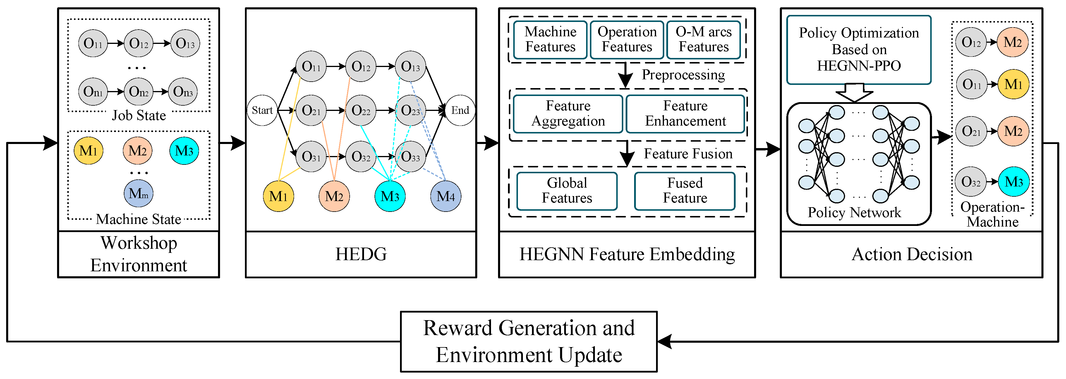
• This study introduces the HEDG structure for modeling the FJSP. The HEDG captures both the precedence constraints and the compatibility between operations and machines, enabling dynamic, real-time updates of scheduling states. This dynamic feature enhances traditional static models, making the framework adaptable to changing production environments and real-time scheduling decisions.
• A heterogeneous enhanced graph neural network (HEGNN) architecture is proposed to extract rich feature representations from the HEDG. By effectively capturing the complex interactions and dependencies between operations and machines, the HEGNN enhances the feature representation, providing deep insights into the scheduling state. This leads to improved decision-making for both operation assignment and machine selection.
• The integration of HEGNN with the PPO algorithm allows for joint optimization of both operation assignment and machine selection. This end-to-end learning framework adapts dynamically, avoiding the pitfalls of local optima that are common in traditional rule-based methods. The method’s effectiveness is further validated through its ability to handle various FJSP instances with different production scales, confirming its practical applicability in real-world industrial settings.

The remainder of this paper is structured as follows. Section 2 formulates the FJSP, including problem definitions, assumptions, and mathematical modeling. Section 3 introduces the proposed HEDG, describes the MDP framework and details the architecture of the HEGNN and its integration with the PPO algorithm for scheduling policy learning. Section 4 presents experimental validation, including instance design, comparative analysis, and performance evaluation. Finally, Section 5 concludes the study and outlines future research directions.

2. Problem Formulation

2.1. Problem Definition and Assumptions

In the context of the FJSP, we consider $n$ jobs that need to be processed on $m$ machines. The set of jobs is denoted as $J=\{J_1,J_2,\dots ,J_n\}$, and the set of machines is represented as $M=\{M_1,M_2,\dots ,M_m\}$. Each job $J_i$ comprises a sequence of operations that must be executed in a specific order, denoted by the set $O_i$. Each operation $O_{ij}$ can be processed on a subset of eligible machines $M_{ij}\subseteq M$.

The scheduling process involves assigning each operation to an appropriate machine and sequencing the operations on each machine to determine the start time $S_{ij}$ for each operation $O_{ij}$. The objective is to establish a comprehensive schedule that minimizes the makespan, defined as the maximum completion time across all jobs [34].

The proposed model is based on the following assumptions:

(1)

Completeness of Job Processing: Every job must complete all its constituent operations.

(2)

Non-Interruptibility and No Rework: Once a job starts processing, it cannot be interrupted or subjected to rework.

(3)

Precedence Constraints: There are strict precedence relations between different operations within the same job, enforcing a specific execution order.

(4)

Machine Assignment: Each operation must be processed on one and only one assigned machine.

(5)

Deterministic Processing Times: The processing time for each operation is fixed and known in advance for each eligible machine.

(6)

Inclusive Setup Times: The setup times required for each operation are encompassed within the processing times.

(7)

Machine Exclusivity: At any given moment, a machine can process only one operation.

2.2. Mathematical Model Building

Based on the problem description and underlying assumptions, we establish a mathematical model for the FJSP. First, we define and describe the parameters used in the model as presented in

Table 2. Definition of the model parameters.

Parameters	Definitions
$i$	$\mathrm{Index} \mathrm{set} \mathrm{of} \mathrm{the} \mathrm{jobs}, i=\mathrm{1,2},\dots ,n$
$j$	$\mathrm{Index} \mathrm{set} \mathrm{of} \mathrm{the} \mathrm{operations}, j=\mathrm{1,2},\dots ,o$
$k$	$\mathrm{Index} \mathrm{set} \mathrm{of} \mathrm{the} \mathrm{machines}, k=\mathrm{1,2},\dots ,m$
$p_{ijk}$	$\mathrm{Processing} \mathrm{time} \mathrm{of} \mathrm{operation} O_{ij}$$\mathrm{on} \mathrm{machine} M_k$
$C_{ij}$	$\mathrm{Completion} \mathrm{time} \mathrm{of} \mathrm{operation} O_{ij}$
$C_{max}$	Makespan (maximum completion time across all jobs)
$S_{ij}$	$\mathrm{Start} \mathrm{time} \mathrm{of} \mathrm{operation} O_{ij}$
$x_{ijk}$	$\mathrm{Binary} \mathrm{decision} \mathrm{variable}: x_{ijk}=1$ $\mathrm{if} \mathrm{operation} O_{ij}$ $\mathrm{is} \mathrm{processed} \mathrm{on} \mathrm{machine} M_k$, 0 otherwise
$y_{ij{i}^{\prime }{j}^{\prime }k}$	$\mathrm{Binary} \mathrm{decision} \mathrm{variable}: y_{ij{i}^{\prime }{j}^{\prime }k}=1$ $\mathrm{if} \mathrm{operation} O_{ij}$ $\mathrm{precedes} O_{ij}$ $\mathrm{on} \mathrm{machine} M_k$, 0 otherwise
$D_i$	$\mathrm{Due} \mathrm{date} \mathrm{of} \mathrm{job} J_i$
${Pr}_i$	$\mathrm{Priority} \mathrm{of} \mathrm{job} J_i$ based on due date urgency
$t$	Current time, representing a specific time point in the scheduling process

.

To minimize the production cycle and achieve more efficient scheduling, the objective is set to minimize the maximum completion time across all jobs. The objective function is formulated as follows:

$$\mathrm{m}\mathrm{i}\mathrm{n} C_{max}=\mathrm{m}\mathrm{i}\mathrm{n}\left(max\right\{C_{ij}\left\}\right)$$

(1)

The constraints of the mathematical model are defined as follows:

$${\displaystyle \sum _{k=1}^m}{x}_{ijk}=1\hspace{1em}\forall i,j$$

(2)

$${\displaystyle \sum _{i-1}^n}{\displaystyle \sum _{j-1}^J}{x}_{ijk}\le 1,\forall k$$

(3)

$$S_{ij}+x_{ijk}\cdot p_{ijk}\le C_{ij},\forall i,j,k$$

(4)

$$C_{ij}\le S_{i\left(j+1\right)},\forall i,j$$

(5)

$$C_{ij}\le C_{max},\forall i,j$$

(6)

$${Pr}_i={\displaystyle \frac{1}{D_i-t}},\forall i$$

(7)

Equation (2) ensures that each operation is uniquely assigned to one machine. Equation (3) maintains that each machine handles only one operation at a time. Equation (4) guarantees that the completion time of each operation accounts for its processing duration. Equation (5) enforces the sequential processing of operations within the same job. Equation (6) ties all operations to the overarching objective of minimizing the maximum completion time. Equation (7) establishes a dynamic priority system for jobs based on their proximity to due dates.

3. Method

To effectively address the FJSP in multi-variety and variable batch production environments, this study presents an intelligent scheduling approach that integrates GNNs with DRL. The proposed method models the FJSP as an MDP, designs a HEGNN architecture, and leverages the Proximal Policy Optimization algorithm to model the scheduling process and optimize decision-making.

As illustrated in Figure 1, the approach begins by constructing an HEDG based on the original workshop environment to effectively represent the shop floor state. The disjunctive graph data are then fed into the HEGNN for node feature embedding. During feature embedding, initial feature preprocessing is performed to ensure data consistency and establish a foundation for subsequent analysis. Subsequently, graph convolution is employed to aggregate and extract deep features from the graph nodes, and an attention mechanism is applied to enhance these features, thereby capturing the intricate relationships between operations and machinery. Finally, global feature representations are obtained through mean pooling of the updated node embeddings. The combination of global and local features serves as the basis for the decision-making and training updates within the PPO algorithm, ultimately achieving optimized scheduling decisions.

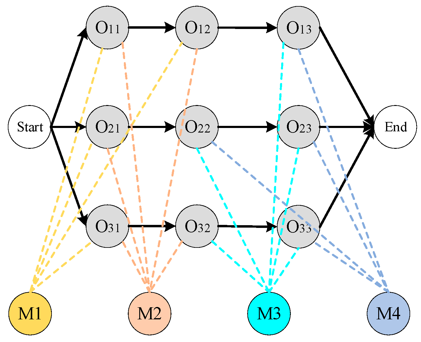
3.1. Heterogeneous Enhanced Disjunctive Graph Model

The disjunctive graph is an effective tool for modeling job shop scheduling processes, commonly used to represent scheduling states, and has achieved significant success [35]. However, in the FJSP, where operations can be processed on multiple machines, the set of disjunctive arcs can become exceedingly large. This results in a densely connected graph topology, complicating the construction of the disjunctive graph [36]. Additionally, the processing time of the same operation may vary across different machines, further increasing the complexity of the graph representation.

In this study, we propose an HEDG model, as illustrated in Figure 2. The model is defined as $H=(O,M,C,G)$, where:

• $O=\{O_{ij}\mid \forall i,j\}\cup \{\mathrm{S}\mathrm{t}\mathrm{a}\mathrm{r}\mathrm{t},\mathrm{E}\mathrm{n}\mathrm{d}\}$ includes all operation nodes and two virtual operation nodes representing the start and end points of the scheduling process (with zero processing time).
• $M=\left\{M_k\right\}$ represents all machines in the workshop.
• $C$ is the set of conjunctive arcs that define the product’s processing routes. For example, the arc $O_{ij}$→$O_{i(j+1)}$ indicates that operation $O_{i(j+1)}$ begins processing after the completion of operation $O_{ij}$.
• $G$ is the set of O−M arcs that connect operation nodes to machine nodes. Each element $G_{ijk}\in G$ is an undirected arc connecting operation node $O_{ij}$ with a selectable machine node $M_k$.

Based on the above definitions, this study represents each state $s_t$ as an HEDG $H_t=(O,M,C,G_t)$, as illustrated in Figure 3. In this framework, $G_t$ dynamically evolves throughout the solution process. When an action $(O_{ij},M_k)$ is executed at time $t$, the arc $G_{ijk}$ is retained, and the other O−M arcs associated with $O_{ij}$ are removed, resulting in the subsequent state $H_{t+1}$. Consequently, the adjacency relationships between nodes are dynamically altered.

The features of operation nodes ${\alpha }_{ij}\in {\mathbb{R}}^8$ are defined as follows:

(1)

Scheduling Status: Indicates whether the operation has been scheduled (0 or 1).

(2)

Number of Adjacent machines: The number of available machines that can be selected for processing.

(3)

Number of Unscheduled Operations: The count of subsequent unscheduled operations within the current job.

(4)

Proportion of Unscheduled Operations: The ratio of unscheduled operations to the total number of operations in the current job.

(5)

Priority: The priority of the job defined based on the delivery date as ${Pr}_i={\displaystyle \frac{1}{D_i-t}}$.

(6)

Processing Time: If scheduled, this is the actual processing time $p_{ijk}$; otherwise, it is the estimated average processing time ${\overline{p}}_{ij}$, calculated as the average processing time across all available machines.

(7)

Start Time: The estimated or actual start time during partial scheduling. If operation $O_{ij}$ has been scheduled, $S_{ij}(t)$ represents the actual start time. If $O_{ij}$ has not been scheduled, the start time is predicted based on the status of preceding operations and available machines. Specifically, if the preceding operation $O_{i(j-1)}$ has started processing on machine $M_k$, then $S_{ij}(t)=S_{i(j-1)}+p_{i(j-1)k}$. Otherwise, the estimated average processing time ${\overline{p}}_{ij}$ is used for prediction.

(8)

Job Completion Time: The estimated or actual completion time during partial scheduling. If operation $O_{ij}$ has been scheduled, the completion time is $C_{ij}(t)=S_{ij}+p_{ijk}$. If $O_{ij}$ has not been scheduled, the completion time is predicted as $C_{ij}(t)=S_{ij}(t)+{\overline{p}}_{ij}$, where $S_{ij}(t)$ is the estimated start time and ${\overline{p}}_{ij}$ is the average processing time.

The features of machine nodes ${\beta }_k\in {\mathbb{R}}^3$ is defined as follows:

(1)

Available Time: The time at which the machine becomes available after completing all currently scheduled operations.

(2)

Number of Adjacent Operations: The number of operations that the machine is capable of processing.

(3)

Utilization: The ratio of the machine’s operating time to the total elapsed time, ranging between 0 and 1.

The features of O−M arcs ${\gamma }_{ijk}\in \mathbb{R}$ are defined as follows:

(1)

Processing Time: The processing time $p_{ijk}$ of operation $O_{ij}$ on machine $M_k$.

The proposed HEDG structure reduces the scale of deduction arcs and simplifies the topological complexity of the graph by introducing machine nodes and undirected arcs connecting machine nodes with process nodes. This approach streamlines the construction process of the deduction graph while incorporating the original features of machine nodes, process nodes, and undirected arcs separately. Consequently, it enhances the graph’s expressive power and adaptability, providing rich state information that facilitates more informed and effective scheduling decisions in subsequent stages.

3.2. Markov Decision Process

This study formulates the scheduling process of the FJSP as an MDP to model and optimize the scheduling decision-making process. The MDP provides a mathematical framework to describe an agent’s decision-making in an environment, which is particularly suitable for modeling complex systems with dynamic interactions and state transitions [37,38]. By modeling the FJSP as an MDP, we define key elements such as states, actions, state transitions, and reward functions. This formalization offers a theoretical foundation for optimizing scheduling decisions by addressing task allocation and resource selection.

The scheduling process is divided into a series of discrete decision points. At each decision instant $t$, the agent selects an action ${\mathrm{a}}_t$ based on the current system state $s_t$. This action corresponds to assigning an unscheduled operation to an available machine and determining its processing start time. Subsequently, the system transitions from state $s_t$ to a new state $s_{t+1}$, and a corresponding reward $r_t$ is generated. This cycle repeats continuously until all operations are completed, signaling the end of the scheduling process.

State: the state $s_t$ encapsulates all relevant information of the system at time step $t$, including the operation status—details such as the start time, completion time, status (scheduled or unscheduled), and dependencies between operations; machine status: information about each machine’s availability time and utilization rate. These components collectively constitute a comprehensive description of the system’s state at time step $t$, providing the agent with a complete view of the system.

Action: The action ${\mathrm{a}}_t$ is the scheduling decision made by the agent at decision instant $t$, defined as an operation–machine pair $(O_{ij},M_k)$, where $M_k$ represents an available machine and $O_{ij}$ denotes an operation pending scheduling. The action set dynamically changes at each decision point, encompassing all feasible operation–machine pairs. By selecting appropriate actions, the agent can effectively allocate resources and optimize the scheduling process.

State Transition: The state transition describes the change from state $s_t$ to state $s_{t+1}$, determined by the current state $s_t$ and the chosen action ${\mathrm{a}}_t$. In the context of the FJSP, state transitions are deterministic, which makes the dynamic evolution of the scheduling process clear and predictable, thereby providing a stable environment for the agent’s learning and decision-making.

Reward: The reward $r_t$ measures the contribution of the action ${\mathrm{a}}_t$ chosen by the agent at time step $t$ towards the scheduling objective. In this study, the reward is defined as the change in the maximum completion time between two consecutive states, i.e., $r_t=C_{max}\left(s_t\right)-C_{max}\left(s_{t+1}\right)$, where $C_{max}\left(s_t\right)$ represents the current makespan under the scheduling scheme. This reward mechanism incentivizes the agent to minimize the makespan, thereby enhancing scheduling efficiency and achieving the optimization goal.

Policy: The policy $\pi \left(a_t\right|s_t)$ defines the probability distribution over actions ${\mathrm{a}}_t$ given the current state $s_t$. Utilizing deep reinforcement learning algorithms, the policy $\pi$ is parameterized by a neural network. By continuously optimizing the parameters of the policy network, the agent learns to select optimal actions in various states, thereby maximizing the cumulative reward and effectively solving the FJSP.

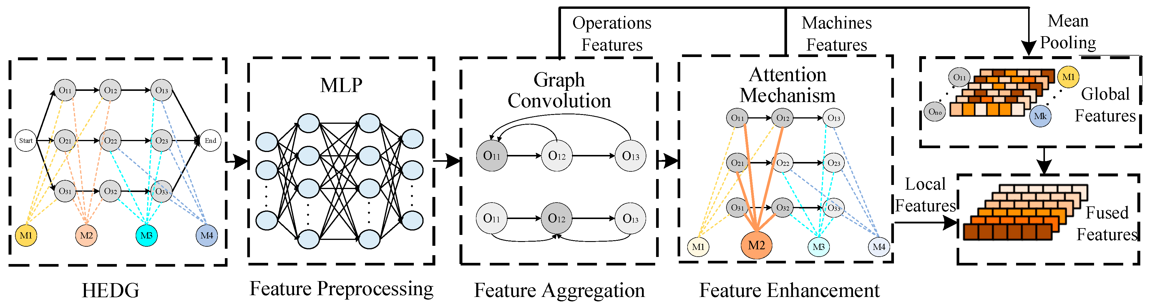
3.3. Heterogeneous Enhanced Graph Neural Network Feature Embedding Framework

To effectively capture the complex interaction information and dependencies within the disjunctive graph, and to provide an informational basis for subsequent scheduling decisions, this paper designs an HEGNN architecture, as illustrated in Figure 4. This framework enables deep representation of the scheduling state through multi-stage feature extraction and fusion:

(1)

Feature Preprocessing: The features of operation nodes and machine nodes are normalized and enhanced to eliminate dimensional differences among feature dimensions. This step improves the representational capability of the features.

(2)

Node Feature Aggregation: Using graph convolutional operations, the framework aggregates the neighboring features of operation nodes, capturing the local structural information among nodes and updating the feature representation of the nodes.

(3)

Attention-Based Feature Enhancement: A multi-head attention mechanism is introduced to dynamically adjust the weights of machine nodes in aggregating the features of operation nodes. This enhances the model’s ability to capture complex relationships.

(4)

Feature Fusion: After extracting local features, global pooling operations are performed to extract global features. These local and global features are then fused to provide more comprehensive feature support for scheduling decisions.

3.3.1. Feature Preprocessing

To mitigate the impact of dimensional differences among various features on the learning process and to enhance the expressive power of the features, normalization and feature enhancement are applied to the features of operation nodes and machine nodes. Initially, the Min–Max normalization method is employed to scale the feature values to the range (0,1), as shown in the following formulas:

$${\alpha }_{ij}^{\mathrm{n}\mathrm{o}\mathrm{r}\mathrm{m}}={\displaystyle \frac{{\alpha }_{ij}-min\left(\alpha \right)}{max\left(\alpha \right)-min\left(\alpha \right)}}$$

(8)

$${\beta }_k^{\mathrm{n}\mathrm{o}\mathrm{r}\mathrm{m}}={\displaystyle \frac{{\beta }_k-min\left(\beta \right)}{max\left(\beta \right)-min\left(\beta \right)}}$$

(9)

Here, $min\left(\alpha \right)$ and $max\left(\alpha \right)$ represent the minimum and maximum values of the feature vector ${\alpha }_{ij}$ for operation nodes, while $min\left(\beta \right)$ and $max\left(\beta \right)$ denote the minimum and maximum values of the feature vector ${\beta }_k$ for machine nodes. This normalization process optimizes the scale and distribution of the features, enhancing the stability of model training and reducing learning biases caused by differences in feature scales [39].

Following normalization, an MLP is introduced to perform nonlinear transformations and dimensional expansion on the features to further enhance their expressive capability:

$${\alpha }_{ij}^{\mathrm{n}\mathrm{o}\mathrm{r}\mathrm{m}}={\displaystyle \frac{{\alpha }_{ij}-min\left(\alpha \right)}{max\left(\alpha \right)-min\left(\alpha \right)}}$$

(10)

$${\beta }_k^{\mathrm{n}\mathrm{o}\mathrm{r}\mathrm{m}}={\displaystyle \frac{{\beta }_k-min\left(\beta \right)}{max\left(\beta \right)-min\left(\beta \right)}}$$

(11)

The MLP design consists of two hidden layers, each followed by a ReLU activation function, with an output dimension of $d_{\mathrm{h}\mathrm{i}\mathrm{d}\mathrm{d}\mathrm{e}\mathrm{n}}$. Through the nonlinear transformations of the MLP, the expressive power of the features is significantly enhanced, providing richer information for subsequent graph convolution operations [40].

3.3.2. Node Feature Aggregation

In GNNs, the interaction and information transfer between nodes are crucial for uncovering complex relationships. To fully leverage the information from nodes and their neighbors, graph convolution operations are widely used for feature extraction. By aggregating the features of each node’s neighbors, graph convolution effectively captures local structural information between nodes and updates the feature representations of the nodes [41]. The specific formula is as follows:

$$H^{(l+1)}=\mathrm{R}\mathrm{e}\mathrm{L}\mathrm{U}\left({\tilde{D}}^{-{\displaystyle \frac{1}{2}}}\tilde{A}{\tilde{D}}^{-{\displaystyle \frac{1}{2}}}{H}^{\left(l\right)}{W}^{\left(l\right)}\right)$$

(12)

Here, $H^{\left(l\right)}$ is the feature matrix of nodes at layer $l$, with dimensions $N\times D_l$, where $N$ is the number of nodes and $D_l$ is the feature dimension at that layer. $W^{\left(l\right)}$ is the weight matrix for layer $l$, used for linear transformations. $\tilde{A}=A+I$ is a modified version of the adjacency matrix $A$, which adds the identity matrix $I$ to ensure that each node is connected to itself. $\tilde{D}$ is the degree matrix of $\tilde{A}$, used for normalization to balance the influence of node degrees.

By aggregating the neighbor features of operation nodes through graph convolution, local structural information between nodes is captured, and the feature representations of the nodes are updated, providing support for subsequent optimization and decision-making.

3.3.3. Attention Feature Enhancement

To better simulate the competitive process between different operations for machines in a real production environment, a multi-head attention mechanism is introduced to update the features of machine nodes. This mechanism dynamically adjusts the weights of feature aggregation to capture the competitive relationships between operation nodes [42]. The core of the attention mechanism lies in calculating the importance weights of each operation node concerning the machine node $M_k$. The feature update formula for the machine node is as follows:

$${\beta }_k^{(l+1)}=\mathrm{R}\mathrm{e}\mathrm{L}\mathrm{U}\left(\sum _{i,j\in N\left(M_k\right)}{\alpha }_{ijk}^{\left(h\right)}\cdot W^{(l,h)}\cdot {\alpha }_{ij}^{\left(l\right)}\right)$$

(13)

Here, $N\left(M_k\right)$ denotes the set of operation nodes connected to the machine node $M_k$, ${\alpha }_{ij}^{\left(l\right)}$ is the feature vector of operation node $O_{ij}$ at layer $l$, ${\alpha }_{ijk}^{\left(h\right)}$ is the attention weight calculated by the $h$-th attention head, which measures the importance of operation node $l$ to machine node $l$, and $W^{(l,h)}$ is the weight matrix for the $h$-th attention head at layer $l$.

The calculation formula for the attention weight ${\alpha }_{ijk}^{\left(h\right)}$ is given by

$${\alpha }_{ijk}^{\left(h\right)}={\displaystyle \frac{\mathrm{e}\mathrm{x}\mathrm{p}\left(e_{ijk}^{\left(h\right)}\right)}{\sum _{i^{\prime },j^{\prime }\in N\left(M_k\right)}\mathrm{e}\mathrm{x}\mathrm{p}\left(e_{i^{\prime }{j}^{\prime }k}^{\left(h\right)}\right)}}$$

(14)

where $e_{ijk}^{\left(h\right)}$ is the raw attention score computed based on the features of operation and machine nodes:

$$e_{ijk}^{\left(h\right)}=\mathrm{L}\mathrm{e}\mathrm{a}\mathrm{k}\mathrm{y}\mathrm{R}\mathrm{e}\mathrm{L}\mathrm{U}\left(a^{\left(h\right)\mathrm{\top }}\cdot [W^{(l,h)}\cdot {\beta }_k^{\left(l\right)}\parallel W^{(l,h)}\cdot {\alpha }_{ij}^{\left(l\right)}]\right)$$

(15)

Here, $a^{\left(h\right)}$ is the learnable parameter vector for the $h$-th attention head, and $\parallel$ denotes the vector concatenation operation. Through the multi-head attention mechanism, machine nodes can more effectively aggregate information from important operation nodes, thereby better reflecting decision preferences in actual production. The outputs of multiple heads are finally concatenated or weighted summed to obtain a richer feature representation:

$${\beta }_k^{(l+1)}=\mathrm{C}\mathrm{o}\mathrm{n}\mathrm{c}\mathrm{a}\mathrm{t}({\beta }_k^{(l+\mathrm{1,1})},{\beta }_k^{(l+\mathrm{1,2})},\dots ,{\beta }_k^{(l+1,H)})W^{\mathrm{o}\mathrm{u}\mathrm{t}}$$

(16)

where $H$ represents the number of attention heads, and $W^{\mathrm{o}\mathrm{u}\mathrm{t}}$ is the weight matrix for the output layer.

3.3.4. Feature Fusion

Through graph convolution operations and attention feature enhancement, the features of operation nodes and machine nodes are updated to extract local features. The graph convolution operation captures local structural information between nodes, while the attention mechanism further enhances the ability of machine nodes to aggregate information from important operation nodes.

For operation node $O_{ij}$ and machine node $M_k$, the local feature update formulas are as follows:

$${\alpha }_{ij}^{\prime }=GraphConv\left({\alpha }_{ij}^{enhanced},\mathcal{N}\left(O_{ij}\right)\right){\alpha }_{ij}^{\mathrm{n}\mathrm{o}\mathrm{r}\mathrm{m}}={\displaystyle \frac{{\alpha }_{ij}-min\left(\alpha \right)}{max\left(\alpha \right)-min\left(\alpha \right)}}$$

(17)

$${\beta }_k^{\prime }=Attention({\beta }_k^{enhanced},\{{\alpha }_{ij}^{\prime }\left|\right(i,j)\in \mathcal{N}(M_k\left)\right\})$$

(18)

Here, $\mathcal{N}\left(O_{ij}\right)$ and $\mathcal{N}\left(M_k\right)$ denote the sets of neighbor nodes for operation node $O_{ij}$ and machine node $M_k$, respectively.

After extracting local features, global features are obtained through mean pooling:

$$h_{global}=MeanPool\left(\right\{{\alpha }_{ij}^{\prime }\mid \forall i,j\}\cup \{{\beta }_k^{\prime }\mid \forall k\left\}\right)$$

(19)

where $h_{global}$ is the global state embedding, representing the global features of the current scheduling state and the overall state of the graph.

Finally, the local features and global features are concatenated to generate the final fused feature representation:

$$h_{final}={\alpha }_{ij}^{\prime }\parallel {\beta }_k^{\prime }\parallel h_{global}$$

(20)

where $\parallel$ denotes the feature concatenation operation, and $h_{final}$ is the final fused feature representation.

Through the above four stages, the proposed HEGNN effectively captures complex relationships between operations and machines, dynamically fuses heterogeneous features, and provides high-dimensional semantic information support for subsequent reinforcement learning strategies.

3.4. Scheduling Policy Optimization Algorithm Based on HEGNN-PPO

Based on the feature information extracted by the HEGNN, this paper proposes a deep reinforcement learning algorithm combining PPO. The algorithm generates operation–machine allocation actions through the policy network and evaluates state values using a critic network, achieving end-to-end scheduling decision optimization.

3.4.1. Scheduling Decision

For each actionable operation $a_t=(O_{ij},M_k)$, the operation embedding, machine embedding, and global state are concatenated and input into an MLP to calculate the priority index:

$$P(a_t,s_t)={\mathrm{M}\mathrm{L}\mathrm{P}}_{\omega }\left(h_{final}\right)$$

(21)

where $h_{final}={\alpha }_{ij}^{\prime }\parallel {\beta }_k^{\prime }\parallel h_{global}$, ${\alpha }_{ij}^{\prime }$ is the updated operation node feature, ${\beta }_k^{\prime }$ is the updated machine node feature, and $h_{global}$ is the global feature.

The probability of selecting each action is calculated using the softmax function:

$${\pi }_{\omega }(a_t|s_t)={\displaystyle \frac{\mathrm{e}\mathrm{x}\mathrm{p}\left(P\right(a_t,s_t\left)\right)}{\sum _{a_t^{\prime }\in A_t}\mathrm{e}\mathrm{x}\mathrm{p}(P(a_t^{\prime },s_t))}}\hspace{1em}\forall a_t\in A_t$$

(22)

During the training phase, actions are sampled according to the policy ${\pi }_{\omega }$ to facilitate exploration; during the testing phase, the action with the highest probability (greedy strategy) is selected as the final decision [43].

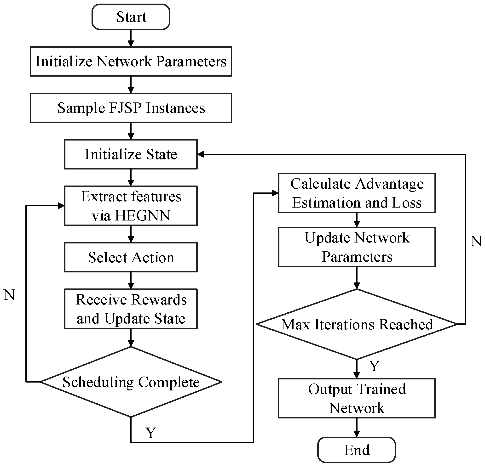
3.4.2. Algorithm Training

The PPO algorithm is used for training, employing an actor–critic architecture [27]. The actor is the policy network ${\pi }_{\omega }$, responsible for generating the probability distribution of actions based on the current state $s_t$; the critic is another network $v_{\varphi }$, which predicts the value $v\left(s_t\right)$ of state $s_t$. The critic network takes the state embedding $h_{global}$ computed by the HEGNN as input and outputs the estimated value of that state.

Policy network update: Using the collected experience data, the PPO algorithm updates the policy network parameters $\omega$ with the objective of maximizing the expected cumulative reward, optimized through the following loss function:

$$L^{\mathrm{c}\mathrm{l}\mathrm{i}\mathrm{p}}\left(\omega \right)={\widehat{\mathbb{E}}}_t\left[min\left({\displaystyle \frac{{\pi }_{\omega }\left(a_t|s_t\right)}{{\pi }_{{\omega }_{\mathrm{o}\mathrm{l}\mathrm{d}}}\left(a_t|s_t\right)}}{\widehat{A}}_t,\mathrm{c}\mathrm{l}\mathrm{i}\mathrm{p}\left({\displaystyle \frac{{\pi }_{\omega }\left(a_t|s_t\right)}{{\pi }_{{\omega }_{\mathrm{o}\mathrm{l}\mathrm{d}}}\left(a_t|s_t\right)}},1-ϵ,1+ϵ\right){\widehat{A}}_t\right)\right]$$

(23)

where ${\widehat{A}}_t$ is the advantage estimate, representing the advantage value of choosing action $a_t$ in state $s_t$, and $ϵ$ is the clipping parameter used to control the extent of policy updates, preventing instability due to overly large updates.

Value network update: The goal of the critic network $v_{\varphi }$ is to minimize the value prediction error, optimized through the following loss function:

$$L^V\left(\varphi \right)={\widehat{\mathbb{E}}}_t\left[\left(v_{\varphi }\right(s_t)-{\widehat{R}}_t{)}^2\right]$$

(24)

where ${\widehat{R}}_t$ is the discounted reward estimate, and ${\widehat{\mathbb{E}}}_t$ denotes the expectation at time step $t$.

The training flowchart of the algorithm is illustrated in Figure 5.

Algorithm 1 outlines the complete training procedure of the proposed HEGNN-PPO scheduling strategy.

Algorithm 1: Training Process

Initialize HEGNN network parameters $\theta$;

Initialize policy network parameters $\omega$;

Initialize critic network parameters $\varphi$;

Sample an initial S of FJSP instances with batch size B;

for i = 1, 2, …, I do:

if i mod 20 == 1 then

sample (B) new FJSP instances;

Initialize the experience buffer D;

for b = 1, 2, …, B do:

Initialize the state $s_t$ based on instance b;

while $s_t$ is not a terminal state do:

Extract features $h_t$ $=\mathrm{HEGNN} \left(s_t\right)$;

Sample action $a_t$ according to the policy ${\pi }_{\omega }(\cdot |h_t)$;

Select action $a_t$, obtain reward $r_t$ and next state $s_{t+1}$;

Store the experience in buffer D;

Update the state $s_t\leftarrow s_{t+1}$;

end while

end for

for k = 1 to K do:

Randomly shuffle D and divide it into batches

Compute the estimated advantages ${\widehat{A}}_t$ and the loss $L$ for each batch;

Update the network parameters $\theta ,$ $\omega$ and $\varphi$;

end for

if i mod 10 = 0 then

evaluate the current policy performance using the validation set;

end if

end for

Output: the trained network parameters;

Based on the algorithm design, the proposed scheduling strategy optimization algorithm effectively leverages the rich feature information extracted by the HEGNN. By integrating the optimization capabilities of the PPO algorithm, it learns high-quality scheduling strategies. This enables efficient and flexible scheduling decisions in complex and dynamic scheduling environments.

4. Experiment

4.1. Experimental Design

To validate the effectiveness of the proposed method, this study constructs five sets of FJSP instances with increasing complexity, based on historical production data from the manufacturing execution system (MES) of a Shanghai-based aerospace company. These instances represent typical production scenarios, encompassing between 10 and 30 jobs and 5 and 10 operations per job, as detailed in

Table 3. Instance scale.

Instance	Number of Jobs	Number of Operations Per Job	Maximum Number of Selectable Machines	Processing Time (h)
S1	10	[5, 10]	[3, 5]	[0.5, 36]
S2	15
S3	20
S4	25
S5	30

.

In real-world production environments, companies typically utilize dispatching rules for production planning. In this study, the proposed method is compared against six composite dispatching rules as well as an existing deep reinforcement learning approach [44]. These six rules encompass three main scheduling objectives: processing time optimization, load balancing, and due date sensitivity, with the specific combinations detailed in

Table 4. Composite dispatching rule.

Composite Dispatching Rule	Descriptions
SPT + NINQ	Shortest Processing Time + Fewest Idle Number of Queues
SPT + WINQ	Shortest Processing Time + Fewest Work in Number of Queues
MWKR + NINQ	Maximum Work Remaining + Fewest Idle Number of Queues
MWKR + WINQ	Maximum Work Remaining + Fewest Work in Number of Queues
EDD + NINQ	Earliest Due Date + Fewest Idle Number of Queues
EDD + WINQ	Earliest Due Date + Fewest Work in Number of Queues

.

The experimental environment is configured with an Intel^® Core™ i5-13400F CPU @ 2.50 GHz, 16 GB of RAM, and an NVIDIA GeForce RTX 3060 Ti 16 GB GPU. During the model architecture design phase, key parameters were inherited from the benchmark configurations presented in reference [42]. The optimal parameter settings were subsequently determined by considering the specific characteristics of the experimental environment, as shown in

Table 5. Model parameter settings.

Parameters	Value
Dimension of node embedding	16
Dimension of the MLP hidden layer	128
Dimension of policy network and value network	64
Number of layers in policy network and value network	3
Number of attention heads	4
Number of iterations	2000
Batch size	20
Discount factor	0.99
Optimizer	Adam
Learning rate	3 × 10⁻⁴
Clipping ratio	0.2
Policy loss coefficient	1
Value loss coefficient	0.5
Exploration strategy	linear decay from 0.5 to 0.1

.

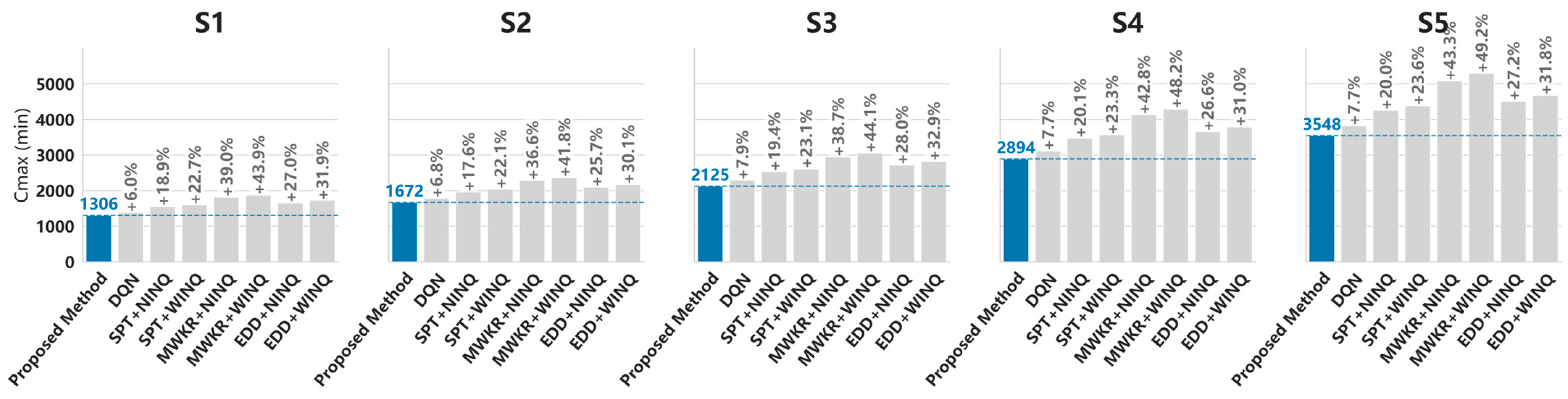
4.2. Experimental Results and Comparison

To validate the effectiveness of the proposed method, the experiments primarily evaluate performance in terms of scheduling quality and response time. The scheduling quality is measured by the makespan $C_{max}$, while the response time refers to the duration required to generate a complete scheduling plan.

As presented in

Table 6. Comparison of scheduling results across instances.

Method	S1	S2	S3	S4	S5
Proposed Method	1306	1672	2125	2894	3548
DQN	1384	1786	2293	3117	3821
SPT + NINQ	1553	1967	2538	3476	4259
SPT + WINQ	1602	2041	2615	3568	4387
MWKR + NINQ	1815	2284	2947	4132	5083
MWKR + WINQ	1879	2371	3062	4289	5295
EDD + NINQ	1658	2102	2719	3664	4512
EDD + WINQ	1723	2176	2825	3791	4678

, the bolded values indicate the optimal makespan results and the proposed method achieved the minimum makespan across all five instances, demonstrating an optimization improvement of 5.6% to 7.3% compared to the DQN method and up to a 35.6% enhancement over traditional composite dispatching rules. This superior performance is attributed to the ability of the HEDG to effectively model the dynamic interactions between operations and machines, as well as the PPO algorithm’s proficiency in learning strategies for global optimization objectives. In contrast, traditional dispatching rules rely on local heuristic strategies, which makes it challenging to capture and manage complex dependencies inherent in the scheduling process.

As shown in

Table 7. Comparison of response times across instances (unit: s).

Method	S1	S2	S3	S4	S5
Proposed Method	0.32	0.63	0.99	1.27	1.9
DQN	0.85	1.12	1.45	1.98	2.35
SPT + NINQ	0.15	0.29	0.42	0.58	0.87
SPT + WINQ	0.15	0.31	0.44	0.6	0.9
MWKR + NINQ	0.16	0.31	0.45	0.6	0.93
MWKR + WINQ	0.16	0.33	0.48	0.65	0.98
EDD + NINQ	0.17	0.35	0.5	0.68	1.05
EDD + WINQ	0.18	0.36	0.52	0.7	1.1

, the proposed method also exhibits favorable response times. Although slightly higher than those of traditional rules, the increase remains modest even as the instance size grows, ensuring that response times scale smoothly with larger problem sizes. Moreover, in practical production environments, these response times are still within acceptable limits. Figure 6 further illustrates that the proposed method achieves an effective balance between scheduling quality and response time, highlighting its practicality and efficiency in real-world manufacturing scenarios.

To further validate the effectiveness of the proposed scheduling method, a detailed performance comparison was conducted using the well-established Brandimarte benchmark dataset [45]. This dataset is widely recognized for evaluating scheduling algorithms and includes 10 problem instances of varying sizes within the FJSP. The dataset serves as a robust test case, reflecting both smaller and larger scale scheduling environments. For this analysis, our method, based on the HEGNN-PPO, was compared with several state-of-the-art methods. The comparison methods include two categories:

DRL-Based Methods:

• AC-SD Method [46]: An end-to-end DRL framework based on an improved pointer network and attention mechanisms, considering both static and dynamic features.
• DRL-AC Method [47]: A reinforcement learning approach based on an actor–critic architecture, utilizing parameterized priority rules and Beta distribution action sampling.

Rule-Based Heuristic Methods:

• Combinations of Shortest Processing Time (SPT + NINQ), Most Work Remaining (MWKR + NINQ), and Earliest Due Date (EDD + NINQ) rules.

The results of this comparison are presented in

Table 8. Performance comparison on the Brandimarte dataset.

Instance	DRL-Based Methods			Rule-Based Heuristic Methods
	Proposed Method	[46]	[47]	SPT + NINQ	MWKR + NINQ	EDD + NINQ
MK01	52	48	45	49	57	55
MK02	34	34	31	43	41	39
MK03	212	235	220	205	234	230
MK04	73	77	72	78	99	78
MK05	182	192	185	184	202	184
MK06	90	121	97	92	114	92
MK07	199	216	210	214	220	214
MK08	528	523	534	541	579	541
MK09	340	375	356	350	397	350
MK10	263	317	283	278	294	278
Average	197.1	213.8	203.3	203.4	223.7	206.1

, which shows the maximum completion time ($C_{max}$) across different scheduling methods for the 10 problem instances. The bolded values indicate the optimal makespan performance. Our model demonstrated competitive performance, achieving the lowest $C_{max}$ in five out of the ten instances (MK05, MK06, MK07, MK09, and MK10). On average, our method achieved a $C_{max}$ of 197.1 h, outperforming the existing DRL-based methods, such as Han et al. [46] and Zhao et al. [47], by 7.8% and 3.1%, respectively. Additionally, our method showed significant improvements when compared to rule-based heuristic methods, with an average optimization of 12.7%.

Despite the overall strong performance, it is worth noting that in the MK08 instance, our method exhibited a slight drop in performance compared to Han et al.’s DRL-based method [46]. This discrepancy is likely due to the specific load balancing challenges in this instance, as MK08 requires careful balancing of machine loads—a factor that our current reward function does not explicitly account for. Future improvements could include incorporating load balancing considerations into the reward structure, which would enhance the performance in such cases.

5. Conclusions

This study addresses the FJSP in multi-product, variable batch production environments by proposing an intelligent scheduling method that integrates HEDGNN with DRL. By constructing an HEDG model, the scheduling states are dynamically represented, leveraging the graph neural network’s capability to deeply extract operation–machine interaction features. Additionally, the PPO algorithm’s policy iteration mechanism facilitates the joint optimization of operation selection and machine assignment decisions. Experimental results, validated in the context of an aerospace structural component processing workshop and the well-established Brandimarte benchmark dataset, demonstrate that the proposed method significantly outperforms traditional dispatching rules and existing DRL approaches. The proposed method balances scheduling optimization and response efficiency, proving its superiority in various scheduling scenarios. Additionally, it consistently achieved competitive results across instances of different sizes, showing improvements over state-of-the-art DRL methods and rule-based heuristics.

This research focuses on scheduling demands within static production environments, primarily addressing resource allocation issues arising from concurrent tasks. However, it does not account for dynamic disturbances such as equipment failures and urgent order insertions, which can impact scheduling stability. Future work should concentrate on dynamic event perception and the design of online rescheduling strategies. By integrating virtual and physical digital technologies, adaptive scheduling systems can be developed to enhance the robustness and practical applicability of scheduling systems in real-world engineering scenarios.

References

1. Zhang, J.; Ding, G.; Zou, Y.; Qin, S.; Fu, J. Review of Job Shop Scheduling Research and Its New Perspectives under Industry 4.0. J. Intell. Manuf. 2019, 30, 1809–1830. [Google Scholar] [CrossRef]
2. Kusiak, A. Smart Manufacturing. Int. J. Prod. Res. 2018, 56, 508–517. [Google Scholar] [CrossRef]
3. Zhang, X.; Ming, X.; Bao, Y. A Flexible Smart Manufacturing System in Mass Personalization Manufacturing Model Based on Multi-Module-Platform, Multi-Virtual-Unit, and Multi-Production-Line. Comput. Ind. Eng. 2022, 171, 108379. [Google Scholar] [CrossRef]
4. Ji, S.; Wang, Z.; Yan, J. A Multi-Type Data Driven Framework for Solving Flexible Job Shop Scheduling Problem Considering Multiple Production Resource States. Comput. Ind. Eng. 2025, 200, 110835. [Google Scholar] [CrossRef]
5. Xie, J.; Gao, L.; Peng, K.; Li, X.; Li, H. Review on Flexible Job Shop Scheduling. IET Collab. Intell. Manuf. 2019, 1, 67–77. [Google Scholar] [CrossRef]
6. Li, J.; Li, H.; He, P.; Xu, L.; He, K.; Liu, S. Flexible Job Shop Scheduling Optimization for Green Manufacturing Based on Improved Multi-Objective Wolf Pack Algorithm. Appl. Sci. 2023, 13, 8535. [Google Scholar] [CrossRef]
7. Gao, K.; Cao, Z.; Zhang, L.; Chen, Z.; Han, Y.; Pan, Q. A Review on Swarm Intelligence and Evolutionary Algorithms for Solving Flexible Job Shop Scheduling Problems. IEEE/CAA J. Autom. Sin. 2019, 6, 904–916. [Google Scholar] [CrossRef]
8. Zheng, P.; Xiao, S.; Zhang, P.; Lv, Y. A Two-Individual-Based Evolutionary Algorithm for Flexible Assembly Job Shop Scheduling Problem with Uncertain Interval Processing Times. Appl. Sci. 2024, 14, 10304. [Google Scholar] [CrossRef]
9. Kong, J.; Yang, Y. Research on Multi-Objective Flexible Job Shop Scheduling Problem with Setup and Handling Based on an Improved Shuffled Frog Leaping Algorithm. Appl. Sci. 2024, 14, 4029. [Google Scholar] [CrossRef]
10. Li, X.; Guo, X.; Tang, H.; Wu, R.; Wang, L.; Pang, S.; Liu, Z.; Xu, W.; Li, X. Survey of Integrated Flexible Job Shop Scheduling Problems. Comput. Ind. Eng. 2022, 174, 108786. [Google Scholar] [CrossRef]
11. Meng, L.; Zhang, C.; Shao, X.; Ren, Y. MILP Models for Energy-Aware Flexible Job Shop Scheduling Problem. J. Clean. Prod. 2019, 210, 710–723. [Google Scholar] [CrossRef]
12. Ortíz, M.A.; Betancourt, L.E.; Negrete, K.P.; De Felice, F.; Petrillo, A. Dispatching Algorithm for Production Programming of Flexible Job-Shop Systems in the Smart Factory Industry. Ann. Oper. Res. 2018, 264, 409–433. [Google Scholar] [CrossRef]
13. Lv, Q.H.; Chen, J.; Chen, P.; Xun, Q.F.; Gao, L. Flexible Job-Shop Scheduling Problem with Parallel Operations Using Reinforcement Learning: An Approach Based on Heterogeneous Graph Attention Networks. Adv. Prod. Eng. Manag. 2024, 19, 157–181. [Google Scholar] [CrossRef]
14. Zhang, C.; Song, W.; Cao, Z.; Zhang, J.; Tan, P.S.; Chi, X. Learning to Dispatch for Job Shop Scheduling via Deep Reinforcement Learning. In Proceedings of the Advances in Neural Information Processing Systems, Vancouver, BC, Canada, 6–12 December 2020; Curran Associates, Inc.: Red Hook, NY, USA, 2020; Volume 33, pp. 1621–1632. [Google Scholar]
15. Chen, B.; Matis, T.I. A Flexible Dispatching Rule for Minimizing Tardiness in Job Shop Scheduling. Int. J. Prod. Econ. 2013, 141, 360–365. [Google Scholar] [CrossRef]
16. Sobeyko, O.; Mönch, L. Heuristic Approaches for Scheduling Jobs in Large-Scale Flexible Job Shops. Comput. Oper. Res. 2016, 68, 97–109. [Google Scholar] [CrossRef]
17. Türkyılmaz, A.; Şenvar, Ö.; Ünal, İ.; Bulkan, S. A Research Survey: Heuristic Approaches for Solving Multi Objective Flexible Job Shop Problems. J. Intell. Manuf. 2020, 31, 1949–1983. [Google Scholar] [CrossRef]
18. Stanković, A.; Petrović, G.; Ćojbašić, Ž.; Marković, D. An Application of Metaheuristic Optimization Algorithms for Solving the Flexible Job-Shop Scheduling Problem. Oper. Res. Eng. Sci. Theory Appl. 2020, 3, 13–28. [Google Scholar] [CrossRef]
19. Kui, C.; Li, B. Research on FJSP of Improved Particle Swarm Optimization Algorithm Considering Transportation Time. J. Syst. Simul. 2021, 33, 845–853. [Google Scholar] [CrossRef]
20. Mei, Z.; Lu, Y.; Lv, L. Research on Multi-Objective Low-Carbon Flexible Job Shop Scheduling Based on Improved NSGA-II. Machines 2024, 12, 590. [Google Scholar] [CrossRef]
21. Heik, D.; Bahrpeyma, F.; Reichelt, D. Study on the Application of Single-Agent and Multi-Agent Reinforcement Learning to Dynamic Scheduling in Manufacturing Environments with Growing Complexity: Case Study on the Synthesis of an Industrial IoT Test Bed. J. Manuf. Syst. 2024, 77, 525–557. [Google Scholar] [CrossRef]
22. Huang, D.; Zhao, H.; Tian, W.; Chen, K. A Deep Reinforcement Learning Method Based on a Multiexpert Graph Neural Network for Flexible Job Shop Scheduling. Comput. Ind. Eng. 2025, 200, 110768. [Google Scholar] [CrossRef]
23. Bouazza, W.; Sallez, Y.; Beldjilali, B. A Distributed Approach Solving Partially Flexible Job-Shop Scheduling Problem with a Q-Learning Effect. IFAC-PapersOnLine 2017, 50, 15890–15895. [Google Scholar] [CrossRef]
24. Chen, R.; Yang, B.; Li, S.; Wang, S. A Self-Learning Genetic Algorithm Based on Reinforcement Learning for Flexible Job-Shop Scheduling Problem. Comput. Ind. Eng. 2020, 149, 106778. [Google Scholar] [CrossRef]
25. Zhang, G.; Lu, X.; Liu, X.; Zhang, L.; Wei, S.; Zhang, W. An Effective Two-Stage Algorithm Based on Convolutional Neural Network for the Bi-Objective Flexible Job Shop Scheduling Problem with Machine Breakdown. Expert Syst. Appl. 2022, 203, 117460. [Google Scholar] [CrossRef]
26. Zhao, Y.; Wang, Y.; Tan, Y.; Zhang, J.; Yu, H. Dynamic Jobshop Scheduling Algorithm Based on Deep Q Network. IEEE Access 2021, 9, 122995–123011. [Google Scholar] [CrossRef]
27. Song, W.; Chen, X.; Li, Q.; Cao, Z. Flexible Job-Shop Scheduling via Graph Neural Network and Deep Reinforcement Learning. IEEE Trans. Ind. Inform. 2023, 19, 1600–1610. [Google Scholar] [CrossRef]
28. Liu, C.-L.; Chang, C.-C.; Tseng, C.-J. Actor-Critic Deep Reinforcement Learning for Solving Job Shop Scheduling Problems. IEEE Access 2020, 8, 71752–71762. [Google Scholar] [CrossRef]
29. Du, Y.; Li, J.; Li, C.; Duan, P. A Reinforcement Learning Approach for Flexible Job Shop Scheduling Problem with Crane Transportation and Setup Times. IEEE Trans. Neural Netw. Learn. Syst. 2024, 35, 5695–5709. [Google Scholar] [CrossRef]
30. Du, Y.; Li, J.; Chen, X.; Duan, P.; Pan, Q. Knowledge-Based Reinforcement Learning and Estimation of Distribution Algorithm for Flexible Job Shop Scheduling Problem. IEEE Trans. Emerg. Top. Comput. Intell. 2023, 7, 1036–1050. [Google Scholar] [CrossRef]
31. He, Z.; Tran, K.P.; Thomassey, S.; Zeng, X.; Xu, J.; Yi, C. Multi-Objective Optimization of the Textile Manufacturing Process Using Deep-Q-Network Based Multi-Agent Reinforcement Learning. J. Manuf. Syst. 2022, 62, 939–949. [Google Scholar] [CrossRef]
32. Tassel, P.; Gebser, M.; Schekotihin, K. A Reinforcement Learning Environment for Job-Shop Scheduling. arXiv 2021. [Google Scholar] [CrossRef]
33. Liu, C.-L.; Huang, T.-H. Dynamic Job-Shop Scheduling Problems Using Graph Neural Network and Deep Reinforcement Learning. IEEE Trans. Syst. Man Cybern. Syst. 2023, 53, 6836–6848. [Google Scholar] [CrossRef]
34. Fattahi, P.; Saidi Mehrabad, M.; Jolai, F. Mathematical Modeling and Heuristic Approaches to Flexible Job Shop Scheduling Problems. J. Intell. Manuf. 2007, 18, 331–342. [Google Scholar] [CrossRef]
35. Park, J.; Chun, J.; Kim, S.H.; Kim, Y.; Park, J. Learning to Schedule Job-Shop Problems: Representation and Policy Learning Using Graph Neural Network and Reinforcement Learning. Int. J. Prod. Res. 2021, 59, 3360–3377. [Google Scholar] [CrossRef]
36. Wang, D.; Liu, S.; Zou, J.; Qiao, W.; Jin, S. Flexible Robotic Cell Scheduling with Graph Neural Network Based Deep Reinforcement Learning. J. Manuf. Syst. 2025, 78, 81–93. [Google Scholar] [CrossRef]
37. Liu, R.; Piplani, R.; Toro, C. A Deep Multi-Agent Reinforcement Learning Approach to Solve Dynamic Job Shop Scheduling Problem. Comput. Oper. Res. 2023, 159, 106294. [Google Scholar] [CrossRef]
38. Jing, X.; Yao, X.; Liu, M.; Zhou, J. Multi-Agent Reinforcement Learning Based on Graph Convolutional Network for Flexible Job Shop Scheduling. J. Intell. Manuf. 2024, 35, 75–93. [Google Scholar] [CrossRef]
39. Zhang, Y.; Zhu, H.; Tang, D.; Zhou, T.; Gui, Y. Dynamic Job Shop Scheduling Based on Deep Reinforcement Learning for Multi-Agent Manufacturing Systems. Robot. Comput.-Integr. Manuf. 2022, 78, 102412. [Google Scholar] [CrossRef]
40. Zhang, W.; Zhao, F.; Li, Y.; Du, C.; Feng, X.; Mei, X. A Novel Collaborative Agent Reinforcement Learning Framework Based on an Attention Mechanism and Disjunctive Graph Embedding for Flexible Job Shop Scheduling Problem. J. Manuf. Syst. 2024, 74, 329–345. [Google Scholar] [CrossRef]
41. Wu, Z.; Pan, S.; Chen, F.; Long, G.; Zhang, C.; Yu, P.S. A Comprehensive Survey on Graph Neural Networks. IEEE Trans. Neural Netw. Learn. Syst. 2021, 32, 4–24. [Google Scholar] [CrossRef]
42. Tang, H.; Dong, J. Solving Flexible Job-Shop Scheduling Problem with Heterogeneous Graph Neural Network Based on Relation and Deep Reinforcement Learning. Machines 2024, 12, 584. [Google Scholar] [CrossRef]
43. Wang, X.; Zhang, L.; Liu, Y.; Zhao, C.; Wang, K. Solving Task Scheduling Problems in Cloud Manufacturing via Attention Mechanism and Deep Reinforcement Learning. J. Manuf. Syst. 2022, 65, 452–468. [Google Scholar] [CrossRef]
44. Luo, S. Dynamic Scheduling for Flexible Job Shop with New Job Insertions by Deep Reinforcement Learning. Appl. Soft Comput. 2020, 91, 106208. [Google Scholar] [CrossRef]
45. Brandimarte, P. Routing and Scheduling in a Flexible Job Shop by Tabu Search. Ann. Oper. Res. 1993, 41, 157–183. [Google Scholar] [CrossRef]
46. Han, B.A.; Yang, J.J. A Deep Reinforcement Learning Based Solution for Flexible Job Shop Scheduling Problem. Int. J. Simul. Model. 2021, 20, 375–386. [Google Scholar] [CrossRef]
47. Zhao, C.; Deng, N. An Actor-Critic Framework Based on Deep Reinforcement Learning for Addressing Flexible Job Shop Scheduling Problems. Math. Biosci. Eng. 2023, 21, 1445–1471. [Google Scholar] [CrossRef]
Figure 1. Scheduling process based on graph neural networks and deep reinforcement learning.
Applsci 15 05648 g001
Figure 2. Structure of the HEDG.
Applsci 15 05648 g002
Figure 3. FJSP scheduling process based on HEDG.
Applsci 15 05648 g003
Figure 4. Feature embedding in HEGNN.
Applsci 15 05648 g004
Figure 5. Training flowchart of the algorithm.
Applsci 15 05648 g005
Figure 6. Comparative visualization of scheduling results.
Applsci 15 05648 g006