Reduction of the Disturbance Effects in a Twin Rotor Multi-Input Multi-Output System Based on a Modified Smith Predictor Control Scheme

Abstract

Three factors that complicate the position and orientation control of unmanned autonomous vehicles are the hardware-induced delays, delays caused by teleoperated modes of operation, and persistent disturbances such as wind. In this article, we study how to overcome these challenges by controlling a twin rotor multi-input, multi-output system. This nonlinear system has two degrees of freedom and significant cross-coupling, making its control particularly challenging. Time delay and external disturbances contribute to system instability and complicate flight control. The effects of time delay can be mitigated using the standard Smith predictor controller. However, this approach performs poorly when persistent disturbances are present. Our contribution is a modified Smith predictor that effectively mitigates disturbances. Additionally, a decoupler is employed to transform the system into two single-input, single-output models, enabling precise control of both the horizontal and vertical planes. The proposed method is implemented on a prototype and compared with the original Smith predictor-based control scheme. Experimental results validate the effectiveness of the proposed approach, showing that our approach reduces the steady-state tracking error to less than 2%, decreases settling time from 30 s to 20 s, and improves disturbance rejection under wind disturbance conditions by 35% compared to the standard Smith predictor. These results demonstrate the superior set-point tracking performance and enhanced disturbance rejection of the proposed approach.

1. Introduction

In recent years, advancements in aerial research have led to various applications that are now part of everyday human life. These applications involve acquiring real-world images in dangerous locations such as active volcanoes, earthquake-prone regions, and wildfire-affected areas, as well as tracking industrial activities and national borders and predicting atmospheric conditions. In reality, these operations can be performed by aircraft and drones, with the twin rotor $MIMO$ system ($TRMS$) being the most commonly used [1,2]. It has encouraged researchers in the control field by serving as a tool for many experiments and enabling real-time adjustments to aeronautical vehicles [2].

In most cases, the $TRMS$ control system is required to accurately measure two angles: pitch and yaw. These are frequently controlled by calculating two ideal $DC$ voltages, where each one supplies power to an individual $DC$ motor [3]. As a result, the system possesses two degrees of freedom, allowing both horizontal and vertical movements. Therefore, the given performance is often restricted by the adequate selection of two main keys [4]. The first key is the determination of a modeling strategy that produces an accurate multi-input, multi-output model ($MIMO$). The second key is the correct choice of a controller synthesis technique.

On this topic, a novel evolutionary proportional–integral–derivative ($PID$) controller design for $TRMS$ using a simplified genetic algorithm was presented [5]. The proposed controller achieves a good response and excellent performance on the $MIMO$ $TRMS$ system. In [6], the behavior dynamics of the $TRMS$ system was decoupled into two single-input, single-output ($SISO$) systems. Each unit is controlled separately using time-optimal, robust $SISO$ regulators. The cross-coupling impact is regarded as a disturbance or the change of system parameters. In this approach, each $SISO$ regulator guarantees an optimal Nyquist plot ($NP$) margin against these uncertainties. Later, various traditional control methods and advanced control techniques were applied [7] to the $MIMO$ $TRMS$ system. These techniques ensure that the $TRMS$ beam moves rapidly and precisely, enabling it to track a trajectory and reach specific positions. A fuzzy $PID$ control scheme was proposed in [8] for $TRMS$, in which a new control structure allows the $TRMS$ to achieve a target position more efficiently than previously. All the gain values of the $PID$ regulator are obtained by the real coded genetic algorithm ($RGA$) with the system performance index as a fitness function. A feedback model predictive control strategy was proposed in [9] for the nonlinear $TRMS$, in which the control scheme makes the $TRMS$ beam move rapidly and precisely to the target positions (pitch and yaw angles). In addition, its structure was tested under disturbance, where an external force was manually applied to the system to assess its performance under significant disturbance conditions. It is evident that the yaw and pitch angles shift from their intended positions due to the applied external force. However, the control system successfully restores stability, ensuring the beam returns to its desired angles. In [10], a decoupled compensator was designed for a physical $TRMS$ by decoupling its actual behavior using a minimal open-loop decoupler. The resulting decoupled $SISO$ units are adjusted using two independent two degrees of freedom ($2DOF-SISO$) controllers, ensuring reference tracking dynamics while maintaining closed-loop robustness and mitigating the cross-coupling effect.

In a recent study, Ref. [11] introduced a linear quadratic regulator ($LQR$) with an integral controller, resulting in a novel robust $LQI$ controller. The effectiveness of this controller was evaluated against several existing controllers from the literature, and its performance was validated through experimental testing. Later, Ref. [12] developed a robust controller by integrating a sliding mode control ($SMC$) approach with a backstepping controller. The backstepping control scheme eliminates the chattering and oscillation issues typically associated with ($SMC$), and the resulting controller is capable of providing excellent reference tracking dynamics for both the pitch and yaw angles, even when accounting for parametric model uncertainties. A control scheme established on active disturbance rejection control and input shaping was proposed in [13] for the $TRMS$. The control objectives involved accurately following the desired trajectories and ensuring disturbance rejection in both the horizontal and vertical planes. Additionally, the composite control demonstrated robustness against changes in system parameters, including variations in the natural frequency and damping ratio. In [14], two robust $SISO$ fractional-order regulators ($FO-PID$) were proposed, in which the control of the pitch angle is completely independent from the control of the yaw angle. A fractional order integral–proportional derivative ($FOI-PD$) controller was simulated and trialed to control each rotor of the $TRMS$ in [15]. The approach achieved enhanced disturbance rejection compared to the standard proportional integral derivative ($PID$) controller and proportional derivative ($PD$) controller. The controller parameters were optimized using the MATLAB^® function fmincom. A robust $2-DOF$ controller was proposed in [16] for the $TRMS$, which had been previously separated into two $SISO$ systems. This controller contains a fractional-order precompensator to ensure accurate reference path tracking behavior and a fractional post-compensator to enhance the closed-loop robustness.

The adaptive explicit nonlinear model predictive control ($AENMPC$) method introduced in [17] was applied to the $TRMS$ considering a strongly coupled nonlinear $MIMO$ system with uncertain parameters. This approach provides improved control outcomes, including enhanced tracking performance, a smoother control law, and increased energy efficiency. More recently, a combination of proportional integral and proportional-derivative ($PI-PD$) controllers was proposed [18] for $TRMS$, to control the pitch and yaw angles.

Flight systems often experience delays, which can result from various factors, including high-order rotor response, control actuator dynamics, filtering processes, and computational delays [19]. Similarly, for $TRMS$ flight systems that contain the time delay produced by the collection of sensor data [20] or that resulting from the cascading of multiple dynamic components used in the complex system [21], the design of the controller for the flight system becomes a big challenge. All of the above are grouped in what is denoted hardware-induced delays $HID$. Moreover, an additional delay is produced when the $TRMS$ is operated in teleoperated mode. Recent studies in the literature propose controller designs that tackle time delays in flight control, utilizing advanced adaptive control theory, such as integrating the Smith predictor with adaptive controllers [20], adaptive compensators based on observers [22], $H_{\infty }$ controllers, adaptive podcast controllers [23], and robust adaptive controllers [24]. In these investigations, the degradation of the flying quality due to the time delay of the systems is considered, and the difficulty in controlling them is apparent.

Persistent disturbances such as wind introduce errors in the position and orientation of $TRMSs$ [13]. Controllers designed not only for positioning and orientation but also for disturbance rejection tend to be more complex to tune [25], and the inherent time delay of the $TRMS$ often leads to control failures [21,26]. To address these challenges, we aim to design a robust controller capable of mitigating the effects of disturbances and compensating for time delays.

The Smith predictor control scheme $SP$ is effective at eliminating the effect of time delay in a closed-loop system [27]. However, its performance degrades when it is required to reject persistent disturbances. Thus, the main contribution of this paper is a modified Smith predictor controller specifically tailored to our $TRMS$, which is effectively represented by a high-order dynamic model with time delay. The proposed controller is designed to accurately track the pitch and yaw angles in the $TRMS$, while compensating for delay and rapidly rejecting disturbances.

Few studies have proposed $MIMO$ extensions of the $SP$. Among them, most have focused on addressing robustness issues related to varying process parameters (e.g., [28]), while only a few have aimed to improve disturbance rejection. In most cases, the $MIMO$ $SP$ has been combined with a decoupler (e.g., [29,30]), allowing the $MIMO$ control problem to be decomposed into several $SISO$ $SP$ control problems.

Most modifications to the $SP$ aimed at enhancing disturbance rejection have been developed for $SISO$ systems. Consistent with the approach mentioned above, extensions of the $SP$ to $MIMO$ systems typically rely on combining these $SISO$-based modifications with process decouplers. As a result, the disturbance rejection capabilities of the modified $SISO$ $SP$ are inherited by the corresponding $MIMO$ control system.

In previous work [31,32,33], we developed a modified $SP$ specifically designed to mitigate the effects of step disturbances in $SISO$ systems. In this paper, we propose extending this control strategy to the $MIMO$ case to address the control requirements of our $TRMS$.

The most relevant disturbance rejection methods for $SISO$ processes with time delay—including the filtered SP modification, internal model control ($IMC$), and feedforward strategies—were compared in [31] with our proposed $SP$ structure in the context of a second-order plant with time delay. Our $SP$ modification was further compared with several other $SP$ variants (including a sliding mode controller) in [32] for $SISO$ integrating processes with time delay. Additionally, it was benchmarked against the standard $SP$ in the case of a first-order process with time delay in [33] In all these comparisons, our modified $SP$ demonstrated superior disturbance rejection performance. Therefore, we anticipate that the $MIMO$ extension of our modified $SP$ will also outperform $MIMO$ schemes based on other $SISO$ disturbance rejection strategies combined with decouplers.

The remainder of the paper is organized as follows. Section 2 is dedicated to the dynamic model of the $TRMS$. Our proposed control scheme is presented in Section 3. Section 4 provides simulated results of a $TRMS$, while Section 5 presents the experimental results. Finally, Section 6 presents the conclusions.

2. Twin Rotor $\mathbf{MIMO}$ System

2.1. Facility Description

The $TRMS$ used in this study is a laboratory apparatus designed by Feedback Instruments, identified as Model 33-220, which represents the complete $TRMS$ experimental platform. It is a highly nonlinear $MIMO$ system. It is composed of two perpendicular rotors—the main rotor and the tail rotor—positioned on a bar with a counterweight. The main rotor generates a lifting force that enables the bar to rotate in a vertical (pitch) plane, while the tail rotor allows rotation in the horizontal (yaw) plane. A schematic diagram of the $TRMS$ system is shown in Figure 1. Each rotor is driven by a $DC$ motor, and the corresponding angular positions are measured by position sensors attached to the pivot. These sensors provide relative position signals. The pitch and yaw angles are controlled by adjusting the voltages ($u_1$ and $u_2$), which are supplied to the main and tail rotor motors, respectively. MATLAB^®/Simulink is employed in external mode to transmit signals between the $TRMS$ via the Advantech $PCI$-1711 data acquisition card.

2.2. Dynamics of the $TRMS$

The $TRMS$ system composed of two rotors—a main rotor and a tail rotor—is subject to forces such as gravity, thrust, centrifugal force, friction, and disturbance torque, all of which influence the motion of the propellers. To counteract these forces, control inputs are applied via $DC$ motors. In this setup, only the pitch and yaw angles are measured outputs, and maintaining their stability is the primary objective of the controller design. With respect to the mechanical unit, the following nonlinear momentum equation can be derived for the pitch motion (vertical plane) of the $TRMS$:

$$I_1·\ddot{\psi }=M_1-M_{FG}-M_{B.\psi }-M_G$$

(1)

where:

• $\ddot{\psi }$: pitch acceleration.
• $I_1$: moment of inertia of vertical plane.
• $M_1$ = $a_1·{{\tau }_1}^2+b_1·{\tau }_1$: nonlinear static characteristic.
• ${\tau }_1$: the momentum of the main rotor.
• $a_1$, $b_2$: constants.
• $M_{FG}=M_g·sin\left(\psi \right)$: gravity momentum.
• $M_g$: gravity momentum
• $\psi$: pitch angle.
• $M_{B.\psi }=B_{1\psi }·\dot{\psi }+B_{2.\psi }·sin\left(2\psi \right)·{\dot{\varphi }}^2$: friction forces momentum.
• $\dot{\psi }$: pitch velocity.
• $\dot{\varphi }$: yaw velocity.
• $\ddot{\varphi }$: yaw acceleration.
• $B_{1\psi }$, $B_{2.\psi }$: constants.
• $M_G=K_{gy}·M_1·\dot{\varphi }·cos\left(\psi \right)$: gyroscopic momentum.
• $K_{gy}$: gyroscopic momentum of parameter.
• $\varphi$: yaw angle.

The motors and the electrical control circuits mounted on the main and tail rotors are approximated by first-order transfer functions. Accordingly, the rotor momentum of the motor mounted in the main rotor (1), expressed in the Laplace domain, is given by:

$${\tau }_1\left(s\right)={\displaystyle \frac{K_1}{T_{11}·s+T_{10}}}·u_1\left(s\right)$$

(2)

where $K_1$ is the gain of the rotor, $T_{11}$ and $T_{10}$ are coefficients that define the main rotor denominator, and $u_1$ is the voltage (V) applied on the main rotor.

The momentum equation of the $TRMS$ in the horizontal plane (yaw motion) is:

$$I_2·\ddot{\varphi }=M_2-M_{B.\varphi }-M_R$$

(3)

where:

• $\ddot{\varphi }$: yaw acceleration.
• $\varphi$: yaw angle.
• $I_2$: moment of inertia of horizontal plane.
• $M_2$ = $a_2·{{\tau }_2}^2+b_2·{\tau }_2$: nonlinear static characteristic.
• ${\tau }_2$: the momentum of the tail rotor.
• $a_2$, $b_2$: constants.
• $M_{B\varphi }$ = $B_{1\varphi }·\dot{\varphi }$: friction forces momentum.
• $B_{1\varphi }$: a constant.
• $\dot{\varphi }$: yaw velocity.
• $M_r$ = ${\displaystyle \frac{K_c(T_0·s+1)}{T_p·s+1}}·M_1$: cross-reaction momentum.
• $K_c$: cross-reaction momentum gain.
• $T_0$, $T_p$: constants.

After taking the inverse Laplace transform of equation $M_r$ and applying approximations to simplify the transfer function, we consider the case where the dynamic response dominates, i.e., $T_{0}s\gg 1$ and $T_{p}s\gg 1$. Under this assumption, the terms $(T_{0}s+1)$ and $(T_{p}s+1)$ can be approximated as $T_{0}s$ and $T_{p}s$, respectively. This yields the simplified relationship:

$$M_R={\displaystyle \frac{K_c·T_0}{T_p}}·M_1$$

(4)

The rotor momentum of the motor mounted in the tail rotor (3) expressed in the Laplace domain is given as:

$${\tau }_2\left(s\right)={\displaystyle \frac{K_2}{T_{21}.s+T_{20}}}.u_2\left(s\right)$$

(5)

where $K_2$ is the gain of the tail rotor, $T_{21}$ and $T_{22}$ are the coefficients that define the tail rotor denominators, and $u_2\left(s\right)$ is the voltage (V) applied on the tail rotor.

The values of the parameters of the previous equations are given in

Table 1. The parameters of the $TRMS$.

Parameter	Value
Inertia moment relative to the vertical plane ($I_1$)	$6.8\times {10}^{-2}$   (kg · ${\mathrm{m}}^2$)
Inertia moment relative to the horizontal plane ($I_2$)	$2\times {10}^{-2}$   (kg · ${\mathrm{m}}^2$)
Characteristic parameter ($a_1$)	$0.0135$
Characteristic parameter ($b_1$)	$0.0924$
Characteristic parameter ($a_2$)	$0.02$
Characteristic parameter ($b_2$)	$0.09$
Gravity momentum ($M_g$)	0.32 $(\mathrm{N}·\mathrm{m})$
Effect of friction on momentum ($B_{1\psi }$)	$6\times {10}^{-3}$  $(\mathrm{N}·\mathrm{m}·\mathrm{s}/\mathrm{rad})$
Effect of friction on momentum ($B_{2\psi }$)	$1\times {10}^{-3}$  $(\mathrm{N}·\mathrm{m}·{\mathrm{s}}^2/\mathrm{rad})$
Effect of friction on momentum ($B_{1\varphi }$)	$1\times {10}^{-1}$  $(\mathrm{N}·\mathrm{m}·\mathrm{s}/\mathrm{rad})$
Effect of friction on momentum ($B_{2\varphi }$)	$1\times {10}^{-2}$  $(\mathrm{N}·\mathrm{m}·{\mathrm{s}}^2/\mathrm{rad})$
Gyroscopic momentum of parameter ($K_{gy}$)	$0.05$  $(\mathrm{s}/\mathrm{rad})$
Main rotor thrust gain ($K_1$)	$1.1$
Tail rotor thrust gain ($K_2$)	$0.8$
Denominator of the main rotor ($T_{11}$)	$1.1$
Denominator of the main rotor ($T_{10}$)	1
Denominator of the tail rotor ($T_{21}$)	1
Denominator of the tail rotor ($T_{20}$)	1
Cross-momentum effect ($T_p$)	2
Cross-momentum effect ($T_0$)	$3.5$
Cross-coupled momentum gain ($K_c$)	$-0.2$

.

2.3. Nonlinear Dynamic Model

The following state space model depicts the complete dynamics of the nonlinear $TRMS$:

$$\begin{array}{cc}\hfill \dot{x_1}& =x_2,\hfill \\ \hfill \dot{x_2}& ={\displaystyle \frac{a_1}{I_1}}{x}_5^2+{\displaystyle \frac{b_1}{I_1}}{x}_5-{\displaystyle \frac{M_g}{I_1}}sin\left(x_1\right)-{\displaystyle \frac{B_{1·\psi }}{I_1}}{x}_2-{\displaystyle \frac{B_{2\psi }}{I_1}}{x}_4^2·sin\left(2x_1\right)-{\displaystyle \frac{K_{gy}}{I_1}}·cos\left(x_1\right)x_3(a_1·x_5^2+b_1·x_5),\hfill \\ \hfill \dot{x_3}& =x_4,\hfill \\ \hfill \dot{x_4}& ={\displaystyle \frac{a_2}{I_2}}{x}_6^2+{\displaystyle \frac{b_2}{I_2}}{x}_6-{\displaystyle \frac{B_{1·\varphi }}{I_2}}·x_4-{\displaystyle \frac{K_c.T_0}{T_p.I_2}}·(\dot{a_1}·x_5^2+b_1·x_5),\hfill \\ \hfill \dot{x_5}& =-{\displaystyle \frac{T_{10}}{T_{11}}}·x_5+{\displaystyle \frac{k_1}{T_{11}}}·u_1,\hfill \\ \hfill \dot{x_6}& =-{\displaystyle \frac{T_{20}}{T_{21}}}·x_6+{\displaystyle \frac{k_2}{T_{21}}}·u_2.\hfill \end{array}$$

We define the state and input vectors as $\mathbf{x}$ = ${[x_1,x_2,\dots ,x_6]}^T$ and $\mathbf{u}$ = ${[u_1,u_2]}^T$, respectively, where ^(T) means a matrix transpose. Each state represents the following:

$$\begin{array}{cc}\hfill x_1& =\psi :\mathrm{Pitch}\mathrm{angle}.\hfill \\ \hfill x_2& =\dot{\psi }:\mathrm{Pitch}\mathrm{velocity}.\hfill \\ \hfill x_3& =\varphi :\mathrm{Yaw}\mathrm{angle}.\hfill \\ \hfill x_4& =\dot{\varphi }:\mathrm{Yaw}\mathrm{velocity}.\hfill \\ \hfill x_5& ={\tau }_1:\mathrm{Momentum}\mathrm{of}\mathrm{main}\mathrm{rotor}.\hfill \\ \hfill x_6& ={\tau }_2:\mathrm{Momentum}\mathrm{of}\mathrm{tail}\mathrm{rotor}.\hfill \end{array}$$

To obtain the transfer functions of a linearized model of the $TRMS$, we first calculate the equilibrium point ${\mathbf{x}}_0$ = ${[x_{01},x_{02},x_{03},x_{04},x_{05},x_{06}]}^T$ under the assumption of input values $u_1=0$, $u_2=0$. The resulting value is ${\mathbf{x}}_0={[k·\pi ,0,0,0,0,0]}^T$, where k is an integer.

2.4. Transfer Function Model

To calculate the transfer function of the $TRMS$, the nonlinear model has been linearized around the equilibrium point ${\mathbf{x}}_0$ by applying Jacobian linearization:

$$A_{ij}=\left[{\displaystyle \frac{\partial {\dot{x}}_i}{\partial x_j}}\right],B_{ij}=\left[{\displaystyle \frac{\partial {\dot{x}}_i}{\partial u_j}}\right].$$

which gives

$$\begin{array}{cc}\hfill \dot{\mathbf{x}}& =\mathbf{A}·\mathbf{x}+\mathbf{B}·\mathbf{u}\hfill \\ \hfill \mathbf{y}& =\mathbf{C}·\mathbf{x}+\mathbf{D}·\mathbf{u}\hfill \end{array}$$

where $\mathbf{y}={[\psi ,\varphi ]}^T$ represents the pitch and yaw angles, and

$$\begin{array}{cc}\mathbf{A}=\left[\begin{array}{cccccc}0& 1& 0& 0& 0& 0\\ -{\displaystyle \frac{M_g}{I_1}}& -{\displaystyle \frac{B_{1\psi }}{I_1}}& 0& 0& {\displaystyle \frac{b_1}{I_1}}& 0\\ 0& 0& 0& 1& 0& 0\\ 0& 0& 0& -{\displaystyle \frac{B_{1\varphi }}{I_2}}& -{\displaystyle \frac{K_c·T_0·b_1}{T_p·I_2}}& {\displaystyle \frac{b_2}{I_2}}\\ 0& 0& 0& 0& -{\displaystyle \frac{T_{10}}{T_{11}}}& 0\\ 0& 0& 0& 0& 0& -{\displaystyle \frac{T_{20}}{T_{21}}}\end{array}\right],& \mathbf{B}=\left[\begin{array}{cc}0& 0\\ 0& 0\\ 0& 0\\ 0& 0\\ {\displaystyle \frac{K_1}{T_{11}}}& 0\\ 0& {\displaystyle \frac{K_2}{T_{21}}}\end{array}\right]\end{array}$$

Substituting above the values given in Table 1, these matrices become:

$$\begin{array}{ccc}\mathbf{A}=\left[\begin{array}{cccccc}0& 1& 0& 0& 0& 0\\ -4.7059& -0.0882& 0& 0& 1.3588& 0\\ 0& 0& 0& 1& 0& 0\\ 0& 0& 0& -5& 1.6170& 4.5\\ 0& 0& 0& 0& -0.9091& 0\\ 0& 0& 0& 0& 0& -1\end{array}\right],& \mathbf{B}=\left[\begin{array}{cc}0& 0\\ 0& 0\\ 0& 0\\ 0& 0\\ 1& 0\\ 0& 0.8\end{array}\right],& \\ \mathbf{C}=\left[\begin{array}{cccccc}1& 0& 0& 0& 0& 0\\ 0& 0& 1& 0& 0& 0\end{array}\right]& \mathbf{D}=\left[\begin{array}{cc}0& 0\\ 0& 0\end{array}\right]\end{array}$$

Subsequently, the linearized state model is converted into a transfer function matrix:

$$\mathbf{G}\left(s\right)=\mathbf{C}·{(s·{\mathbf{I}}_6-\mathbf{A})}^{-1}·\mathbf{B}+\mathbf{D}=\left[\begin{array}{cc}{G}_{11}\left(s\right)& G_{12}\left(s\right)\\ G_{21}\left(s\right)& G_{22}\left(s\right)\end{array}\right]=\left[\begin{array}{cc}{\displaystyle \frac{1.359}{s^3+0.9973·s^2+4.786·s+4.278}}& 0\\ {\displaystyle \frac{1.617}{s^3+5.909·s^2+4.546·s}}& {\displaystyle \frac{3.6}{s^3+6·s^2+5·s}}\end{array}\right]$$

(6)

where ${\mathbf{I}}_n$ represents the identity matrix of dimensions $nxn$. In this transfer function matrix, $G_{11}\left(s\right)$ is the transfer function in the vertical plane, $G_{22}\left(s\right)$ is the transfer function in the horizontal plane, and $G_{12}\left(s\right)$ and $G_{21}\left(s\right)$ are coupling access transfer functions.

The time delay of our $TRMS$ platform is derived from sensor data and is influenced by the cascading effects of multiple dynamic elements, including the effect of a teleoperated mode. As a result, the same delay is introduced in both input signals $u_1$ and $u_2$. Consequently, the time delay in the $TRMS$ is represented by

$$\mathbf{L}\left(s\right)=\mathrm{diag}\left(e^{-L·s},e^{-L·s}\right)={\mathbf{I}}_2·e^{-L·s}$$

(7)

where $L=0.4$ s.

Finally, the complete linearized model of our $TRMS$ is

$$\widehat{\mathbf{G}}\left(s\right)=\mathbf{G}\left(s\right)·\mathbf{L}\left(s\right)$$

(8)

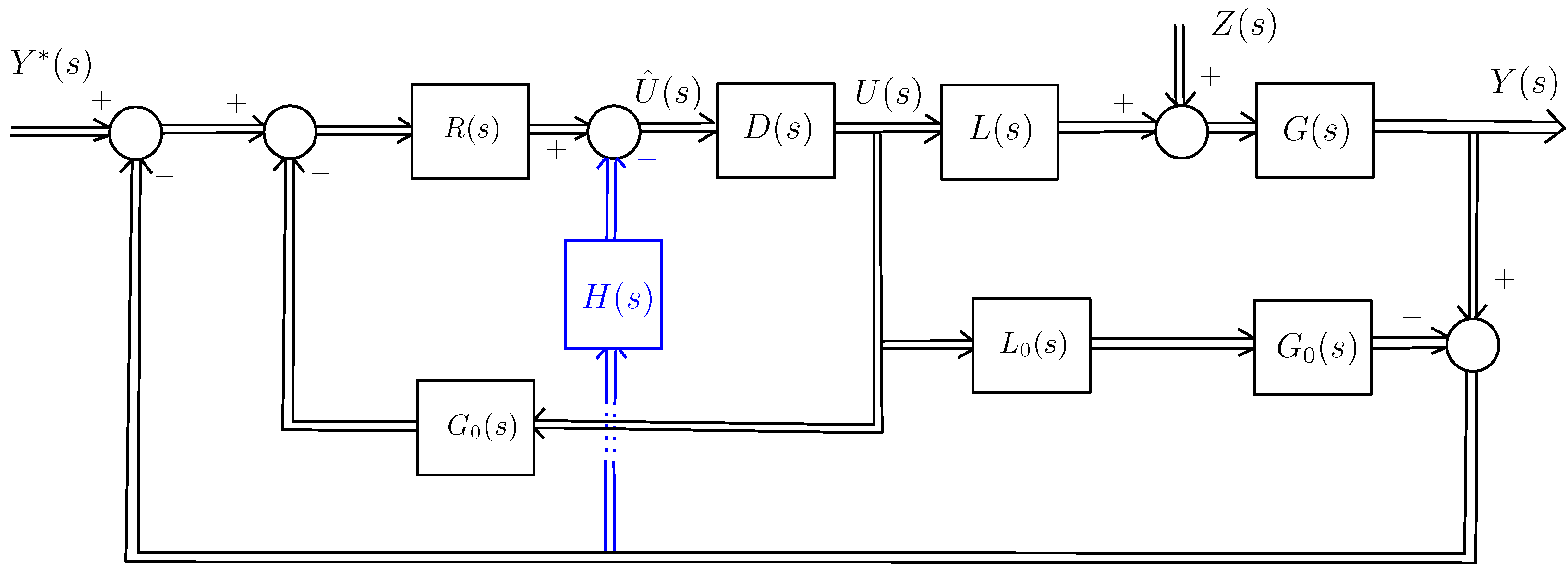
3. Modified Smith Predictor Control Scheme

A modified $SP$ for $TRMS$ is depicted in Figure 2. In this figure, the original $SP$ scheme is illustrated by the black lines and boxes. In this scheme, $G\left(s\right)$ is the actual dynamic model of the $TRMS$, as defined in the Equation (6), while ${\mathbf{G}}_0\left(s\right)$ represents a nominal model of $\mathbf{G}\left(s\right)$, and ${\mathbf{L}}_0\left(s\right)$ represents a nominal time delay model of $\mathbf{L}\left(s\right)$. ${\mathbf{Y}}^{*}\left(s\right)={[{\psi }^{*},{\varphi }^{*}]}^T$ is the reference vector of the system, where ${\psi }^{*}\left(s\right)$ is the reference for the vertical plane (pitch angle), and ${\varphi }^{*}\left(s\right)$ for the horizontal plane (yaw angle). $\mathbf{R}\left(s\right)$ = $diag(R_1\left(s\right),R_2\left(s\right))$ performs the control function and $\mathbf{D}\left(s\right)=[D_{11}\left(s\right),D_{12}\left(s\right);D_{21}\left(s\right),D_{22}\left(s\right)]$ is a decoupler. $\mathbf{U}\left(s\right)={[u_1\left(s\right),u_2\left(s\right)]}^T$ is the control signal vector, where $u_1\left(s\right)$ is the control signal for the vertical plane, and $u_2\left(s\right)$ for the horizontal plane. $\widehat{\mathbf{U}}\left(s\right)={[{\widehat{u}}_1\left(s\right),{\widehat{u}}_2\left(s\right)]}^T$ is the fictitious control signal vector applied to the decoupled system. $\mathbf{H}\left(s\right)$ = $diag([H_1\left(s\right),H_2\left(s\right))$ is the disturbance controller. $\mathbf{Z}\left(s\right)$ = ${[z_1\left(s\right),z_2\left(s\right)]}^T$ is the external disturbance applied to the $TRMS$. $\mathbf{Y}\left(s\right)={[\psi \left(s\right),\varphi \left(s\right)]}^T$ is the response of the system vector, where $\psi \left(s\right)$ is the yaw angle in the vertical plane, and $\varphi \left(s\right)$ in the horizontal plane.

We denote the decoupled system (removing the delay) as $\mathbf{Q}\left(s\right)=\mathbf{G}\left(s\right)·\mathbf{D}\left(s\right)$ and its nominal value as ${\mathbf{Q}}_0\left(s\right)={\mathbf{G}}_0\left(s\right)·\mathbf{D}\left(s\right)$.

3.1. Design of the Main Controller

The main controller is composed of a regulator $\mathbf{R}\left(s\right)$ and a decoupler $\mathbf{D}\left(s\right)$. The design procedures for these two components are outlined next.

• Design of the Decoupler $\mathbf{D}\left(s\right)$
  The decoupler splits the control structure into two subsystems: one controlling the vertical plane and other controlling the horizontal plane. It eliminates the interactions between $u_1$ and $y_2$ and between $u_2$ and $y_1$, allowing each output to be independently regulated by its corresponding input. A simplified decoupling structure, aligned with this tuning approach [34] is employed:

  $$\mathbf{D}\left(\mathbf{s}\right)=\left[\begin{array}{cc}1& -{\displaystyle \frac{G_{0,12}\left(s\right)}{G_{0,11}\left(s\right)}}\\ -{\displaystyle \frac{G_{0,21}\left(s\right)}{G_{0,22}\left(s\right)}}& 1\end{array}\right]=\left[\begin{array}{cc}1& 0\\ {\displaystyle \frac{-17s^3-102s^2-85s}{3.6s^3+21.27s^2+16.37s}}& 1\end{array}\right]$$

  (9)

  where $G_{0,ij}\left(s\right)$ are the elements of the nominal transfer function matrix ${\mathbf{G}}_0\left(s\right)$. Then, we define

  $$\mathbf{Q}\left(s\right)=\mathbf{G}\left(s\right)·\mathbf{D}\left(s\right)=diag\left(Q_1\left(s\right),Q_2\left(s\right)\right)$$

  (10)

  which, in general, is not a diagonal matrix. In the case of the nominal process, we have that

  $${\mathbf{Q}}_0\left(s\right)={\mathbf{G}}_0\left(s\right)·\mathbf{D}\left(s\right)=diag(Q_{0,1}\left(s\right),Q_{0,2}\left(s\right))$$

  (11)

  where $Q_{0,1}\left(s\right)=G_{0,11}\left(s\right)$ and $Q_{0,2}\left(s\right)=G_{0,22}\left(s\right)$. Taking into account the commutative property of the product of diagonal matrices, we have that

  $${\mathbf{G}}_0\left(s\right)·{\mathbf{L}}_0\left(s\right)·\mathbf{D}\left(s\right)={\mathbf{Q}}_0\left(s\right)·e^{-L_0·s}$$

  (12)

  where $L_0$ is the nominal time delay.
• Design of the Regulator $\mathbf{R}\left(s\right)$
  $PID$ controllers are designed in the diagonal elements of $\mathbf{R}\left(s\right)$:

  $$R_i\left(s\right)=K_{P,i}\left(1+{\displaystyle \frac{1}{T_{I,i}·s}}+T_{D,i}·s\right),i=1,2$$

  (13)

  using the nominal process, i.e, $Q_0\left(s\right)$ and $L_0\left(s\right)$.
  Frequency domain techniques are often used to design these controllers. In particular, they are designed using the phase margin ${\theta }_m$ and the gain margin $A_m$, according to [7]:

  $$Q_{0,i}(j·{\omega }_{p,i})·e^{-j·{\omega }_{p,i}·L_0}·\left[K_{P,i}+j·\left(K_{P,i}·T_{D,i}·{\omega }_{p,i}-{\displaystyle \frac{K_{P,i}}{T_{I,i}·{\omega }_{p,i}}}\right)\right]=-{\displaystyle \frac{1}{A_{m,i}}},$$

  (14)

  $$Q_i(j·{\omega }_{g,i})·e^{-j·{\omega }_{g,i}·L_0}·\left[K_{P,i}+j\left(K_{P,i}·T_{D,i}·{\omega }_{g,i}-{\displaystyle \frac{K_{P,i}}{T_{I,i}·{\omega }_{g,i}}}\right)\right]=-e^{-j·{\theta }_{m,i}}.$$

  (15)
  The parameters of the controllers are defined as follows:

  $$\begin{array}{cc}\hfill K_{P,i}& =Re\left({\displaystyle \frac{-1}{A_{m,i}·Q_i(\mathrm{j}·{\omega }_{p,i})·e^{-j·{\omega }_{p,i}·L_0}}}\right),\hfill \end{array}$$

  (16)

  $$\begin{array}{cc}\hfill {\displaystyle \frac{K_{P,i}}{T_{I,i}}}& =\left(X_{p,i}·{\omega }_{g,i}-X_{g,i}·{\omega }_{p,i}\right)·{\left({\displaystyle \frac{{\omega }_{p,i}}{{\omega }_{g,i}}}-{\displaystyle \frac{{\omega }_{g,i}}{{\omega }_{p,i}}}\right)}^{-1},\hfill \end{array}$$

  (17)

  $$\begin{array}{cc}\hfill {\displaystyle \frac{K_{P,i}}{T_{D,i}}}& =\left({\displaystyle \frac{X_{p,i}}{{\omega }_{g,i}}}-{\displaystyle \frac{X_{g,i}}{X_{p,i}}}\right)·{\left({\displaystyle \frac{{\omega }_{p,i}}{{\omega }_{g,i}}}-{\displaystyle \frac{{\omega }_{g,i}}{{\omega }_{p,i}}}\right)}^{-1}\hfill \end{array}$$

  (18)

  where:

  $$\begin{array}{cc}\hfill X_{p,i}& =Im\left({\displaystyle \frac{-1}{A_{m,i}·Q_i(\mathrm{j}·w_{p,i})·e^{-j·{\omega }_{p,i}·L_0}}}\right),\hfill \end{array}$$

  (19)

  $$\begin{array}{cc}\hfill X_{g,i}& =Im\left(-{\displaystyle \frac{e^{\mathrm{j}{\theta }_{m,i}}}{Q_i(\mathrm{j}·w_{g,i})·e^{-j·{\omega }_{g,i}·L_0}}}\right).\hfill \end{array}$$

  (20)
  The specifications of the $R_1\left(s\right)$ controller for the vertical plane are as follows:
  Phase margin: $\varphi ={40}^{\circ }$.
  Phase crossover frequency: $w_g=0.12$ rad/s.
  Gain crossover frequency: $w_p=2.2$ rad/s.
  The specifications of the $R_2\left(s\right)$ controller for the horizontal plane are as follows:
  Phase margin: $\varphi ={40}^{\circ }$.
  Phase crossover frequency: $w_g=0.12$ rad/s.
  Gain crossover frequency: $w_p=2.8$ rad/s.
  These specifications for both the vertical and horizontal plane control of the $TRMS$ were selected to balance stability, robustness, and response speed for the vertical plane control of the $TRMS$. A phase margin of ${40}^{\circ }$ ensures robustness against model uncertainties while avoiding excessive oscillations. The phase crossover frequency ($0.12\mathrm{rad}/\mathrm{s}$) corresponds to a settling time of approximately 26 s, ensuring smooth and stable response. The gain crossover frequency ($2.2\mathrm{rad}/\mathrm{s}$) provides sufficient bandwidth for disturbance rejection while maintaining robustness against high-frequency noise and unmodeled dynamics. Then, the parameters of the controller $\mathbf{R}\left(s\right)$ are the following:

  $$\mathbf{R}\left(\mathbf{s}\right)=\left[\begin{array}{cc}0.0202+0.0602·s+{\displaystyle \frac{0.2816}{s}}& 0\\ 0& 1.8667+0.1146·s+{\displaystyle \frac{0.0151}{s}}\end{array}\right]$$

  (21)

3.2. Standard Smith Predictor

The response of the $TRMS$ using a standard $SP$ is [32,35]:

$$\begin{array}{c}\hfill {\mathbf{Y}}_{SP}\left(s\right)={\mathbf{Y}}_{r_{SP}}\left(s\right)+{\mathbf{Y}}_{d_{SP}}\left(s\right)\end{array}$$

(22)

where ${\mathbf{Y}}_{r_{SP}}\left(s\right)$ represents the relationship between the response output $\mathbf{Y}\left(s\right)$ and the desired reference input ${\mathbf{Y}}^{*}\left(s\right)$, and ${\mathbf{Y}}_{d_{SP}}\left(s\right)$ denotes represents the influence of the disturbance $\mathbf{Z}\left(s\right)$ on $\mathbf{Y}\left(s\right)$. These are provided, respectively, by:

$$\begin{array}{cc}\hfill {\mathbf{Y}}_{r_{SP}}\left(s\right)& ={\displaystyle [}{\mathbf{I}}_2+\mathbf{Q}\left(s\right)·\mathbf{L}\left(s\right)·{\left[{\mathbf{I}}_2+\mathbf{R}\left(s\right)·{\mathbf{Q}}_0\left(s\right)·({\mathbf{I}}_2-{\mathbf{L}}_0\left(s\right))\right]}^{-1}·\mathbf{R}\left(s\right){\displaystyle ]}\hfill \\ \hfill & ·\mathbf{Q}\left(s\right)·\mathbf{L}\left(s\right)·{\left[{\mathbf{I}}_2+\mathbf{R}\left(s\right)·{\mathbf{Q}}_0\left(s\right)·({\mathbf{I}}_2-{\mathbf{L}}_0\left(s\right))\right]}^{-1}·\mathbf{R}\left(s\right)·{\mathbf{Y}}^{*}\left(s\right)\hfill \end{array}$$

(23)

$$\begin{array}{cc}\hfill {\mathbf{Y}}_{d_{SP}}\left(s\right)& =\left[{\mathbf{I}}_2+\mathbf{Q}\left(s\right)·\mathbf{L}\left(s\right)·{\left[{\mathbf{I}}_2+\mathbf{R}\left(s\right)·{\mathbf{Q}}_0\left(s\right)·({\mathbf{I}}_2-{\mathbf{L}}_0\left(s\right))\right]}^{-1}·\mathbf{R}\left(s\right)\right]·\mathbf{Q}\left(s\right)·{\mathbf{D}}^{-\mathbf{1}}\left(s\right)·\mathbf{Z}\left(s\right)\hfill \end{array}$$

(24)

In a nominal situation, where $\mathbf{Q}\left(s\right)$ = ${\mathbf{Q}}_0\left(s\right)$ and $\mathbf{L}\left(s\right)$ = ${\mathbf{L}}_0\left(s\right)$, the previous equations become:

$${\mathbf{Y}}_{r_{SP}}^n\left(s\right)={\left[{\mathbf{I}}_2+\mathbf{R}\left(s\right)·{\mathbf{Q}}_{\mathbf{0}}\left(s\right)\right]}^{-1}·{\mathbf{Q}}_{\mathbf{0}}\left(s\right)·{\mathbf{L}}_0\left(s\right)·\mathbf{R}\left(s\right)·{\mathbf{Y}}^{*}\left(s\right)$$

(25)

$$\begin{array}{cc}\hfill {\mathbf{Y}}_{d_{SP}}^n\left(s\right)& ={\left[{\mathbf{I}}_2+\mathbf{R}\left(s\right)·{\mathbf{Q}}_0\left(s\right)\right]}^{-1}·{\mathbf{\Psi }}_{SP}\left(s\right)·{\mathbf{Q}}_{\mathbf{0}}\left(s\right)·{\mathbf{D}}^{-1}\left(s\right)·\mathbf{Z}\left(s\right)\hfill \end{array}$$

(26)

where

$${\mathbf{\Psi }}_{SP}\left(s\right)={\mathbf{I}}_2+\mathbf{R}\left(s\right)·{\mathbf{Q}}_0\left(s\right)-\mathbf{R}\left(s\right)·{\mathbf{Q}}_0\left(s\right)·{\mathbf{L}}_0\left(s\right)$$

(27)

3.3. Modified Smith Predictor

The innovative structure, based on a modified Smith predictor for controlling the $TRMS$, introduces a compensator $\mathbf{H}\left(s\right)$, whose output is inserted between the $\mathbf{R}\left(s\right)$ and the decoupler $\mathbf{D}\left(s\right)$. Placing H(s) at this point allows it to operate on the decoupled control signals, effectively mitigating external disturbances and modeling uncertainties in both the vertical and horizontal channels. This configuration ensures that disturbance compensation is performed before the cross-coupling dynamics, handled by D(s), are reintroduced, thereby improving the overall robustness and performance of the $TRMS$ control system. This structural modification is represented by the blue lines in Figure 2. The compensator is integrated with the original $SP$ architecture to generate a modified control signal. It will be shown that, for the nominal process, this block affects only the disturbance response while leaving the set-point tracking performance unchanged. Therefore, it can be used reduce the impact of disturbances on the system. The proposed control system, hereafter referred as $SP-H$, was initially designed for a heating furnace modeled as a $SISO$ second-order process with a time delay [31]. It was later adapted to control a marginally stable $DC$ motor (i.e., with a pole at the origin) [32]. In the present work, we have redesigned the control system to handle a high-order $MIMO$ system along with time delays, which characterizes the $TRMS$. Additionally, we examined the benefits of this new $SP$ structure over the standard one in mitigating the effects of wind disturbances on the $TRMS$. The transfer function matrices of the $TRMS$ with the $SP-H$ control scheme are expressed as:

$$\begin{array}{c}\hfill {\mathbf{Y}}_{SP-H}\left(s\right)={\mathbf{Y}}_{r_{SP-H}}\left(s\right)+{\mathbf{Y}}_{d_{SP-H}}\left(s\right)\end{array}$$

(28)

$$\begin{array}{cc}\hfill {\mathbf{Y}}_{r_{SP-H}}\left(s\right)& =[{\mathbf{I}}_2+\mathbf{Q}\left(s\right)·\mathbf{L}\left(s\right)·{\left[{\mathbf{I}}_2+\mathbf{R}\left(s\right)·{\mathbf{Q}}_0\left(s\right)-(\mathbf{R}\left(s\right)+\mathbf{H}\left(s\right))·{\mathbf{Q}}_{\mathbf{0}}\left(s\right)·{\mathbf{L}}_{\mathbf{0}}\left(s\right)\right]}^{-1}\hfill \\ \hfill & ·(\mathbf{R}\left(s\right)+\mathbf{H}\left(s\right))]·\mathbf{Q}\left(s\right)·\mathbf{L}\left(s\right)·{\left[{\mathbf{I}}_2+\mathbf{R}\left(s\right)·{\mathbf{Q}}_0\left(s\right)-(\mathbf{R}\left(s\right)+\mathbf{H}\left(s\right))·{\mathbf{Q}}_{\mathbf{0}}\left(s\right)·{\mathbf{L}}_{\mathbf{0}}\left(s\right)\right]}^{-1}\hfill \\ \hfill & ·\mathbf{R}\left(s\right)·{\mathbf{Y}}^{*}\left(s\right)\hfill \end{array}$$

(29)

$$\begin{array}{cc}\hfill {\mathbf{Y}}_{d_{SP-H}}\left(s\right)& =[{\mathbf{I}}_2+\mathbf{Q}\left(s\right)·\mathbf{L}\left(s\right)·{\left[{\mathbf{I}}_2+\mathbf{R}\left(s\right)·{\mathbf{Q}}_0\left(s\right)-(\mathbf{R}\left(s\right)+\mathbf{H}\left(s\right))·{\mathbf{Q}}_{\mathbf{0}}\left(s\right)·{\mathbf{L}}_{\mathbf{0}}\left(s\right)\right]}^{-1}\hfill \\ \hfill & ·(\mathbf{R}\left(s\right)+\mathbf{H}\left(s\right))]·\mathbf{Q}\left(s\right)·{\mathbf{D}}^{-\mathbf{1}}\left(s\right)·\mathbf{Z}\left(s\right).\hfill \end{array}$$

(30)

In the nominal situation, the above equations become:

$${\mathbf{Y}}_{r_{SP-H}}^n\left(s\right)={\left[{\mathbf{I}}_2+\mathbf{R}\left(s\right)·{\mathbf{Q}}_0\left(s\right)\right]}^{-1}·{\mathbf{Q}}_{\mathbf{0}}\left(s\right)·{\mathbf{L}}_0\left(s\right)·\mathbf{R}\left(s\right)·{\mathbf{Y}}^{*}\left(s\right)$$

(31)

$${\mathbf{Y}}_{d_{SP-H}}^n\left(s\right)={\left[{\mathbf{I}}_2+\mathbf{R}\left(s\right)·{\mathbf{Q}}_0\left(s\right)\right]}^{-1}·{\mathbf{\Psi }}_{SP-H}\left(s\right)·{\mathbf{Q}}_{\mathbf{0}}\left(s\right)·{\mathbf{D}}^{-1}\left(s\right)·\mathbf{Z}\left(s\right)$$

(32)

where

$${\mathbf{\Psi }}_{SP-H}\left(s\right)={\mathbf{I}}_2+\mathbf{R}\left(s\right)·{\mathbf{Q}}_0\left(s\right)-(\mathbf{R}\left(s\right)+\mathbf{H}\left(s\right))·{\mathbf{Q}}_{\mathbf{0}}\left(s\right)·{\mathbf{L}}_{\mathbf{0}}\left(s\right)$$

(33)

Transfer function (31) demonstrates that the set-point tracking performance is influenced solely by $\mathbf{R}\left(s\right)$. In contrast, transfer function (32), (33) is affected by both $\mathbf{R}\left(s\right)$ and $\mathbf{H}\left(s\right)$. Therefore, a careful design of $\mathbf{H}\left(s\right)$ can mitigate the impact of the disturbance $\mathbf{Z}\left(s\right)$ on the output $\mathbf{Y}\left(s\right)$, which would otherwise be present in the standard $SP$ configuration.

3.4. The Disturbance Rejection Controller $H\left(s\right)$

The $H\left(s\right)$ controller serves as the disturbance rejection controller, aimed at mitigating and absorbing the impact of persistent perturbations like the wind effects on the $TRMS$ system [13]. The control scheme of our $SP$ has two subsystems. This is a special feature that allowed us to design a new controller that can remove the disturbance effect that impacts the system. The new controller is based on adding an inner loop that feedbacks the difference between the process output and the nominal model output. In our control scheme, we define $\mathbf{H}\left(s\right)$ as:

$$\mathbf{H}\left(s\right)=\mathbf{F}\left(s\right)·{\mathbf{Q}}_0^{-1}\left(s\right)$$

(34)

where $\mathbf{F}\left(s\right)$ is a diagonal transfer function matrix such that $\mathbf{F}\left(0\right)=\mathbf{I}$. A simple choice of $\mathbf{F}\left(s\right)$ is

$$\mathbf{F}\left(s\right)=\left[\begin{array}{cc}{F}_1\left(s\right)& 0\\ 0& F_2\left(s\right)\end{array}\right],F_1\left(s\right)={\displaystyle \frac{1}{{({\lambda }_{11}·s+1)}^{n_{11}}}},F_2\left(s\right)={\displaystyle \frac{1}{{({\lambda }_{22}·s+1)}^{n_{22}}}}$$

(35)

where $n_{11}$ and $n_{22}$ are chosen as the minima integer values that make the elements of matrix $H\left(s\right)$ proper. Substituting (34) in (33) gives that

$${\mathbf{\Psi }}_{SP-H}\left(s\right)={\mathbf{I}}_2-\mathbf{F}\left(s\right)·{\mathbf{L}}_0\left(s\right)+\mathbf{R}\left(s\right)·{\mathbf{Q}}_0\left(s\right)·({\mathbf{I}}_2-{\mathbf{L}}_0\left(s\right))$$

(36)

which coincides with ${\mathbf{\Psi }}_{SP}\left(s\right)$ when $\mathbf{F}\left(0\right)=\mathbf{I}$ is set.

Comparison of (27) and (36), shows that the difference is that the term ${\mathbf{I}}_2$ of the first equation becomes ${\mathbf{I}}_2-\mathbf{F}\left(s\right)·{\mathbf{L}}_0\left(s\right)$ in the second one. This implies that, if the final value theorem were applied to determine the steady state effect of the disturbance on the output, this term is constant in the first equation while it tends to zero in the second when $\omega \to 0$. This suggests a better disturbance rejection feature of the $SP-H$ at low frequencies than that of the $SP$.

The effect of persistent disturbances on the output is reduced if the magnitudes of ${\mathbf{\Psi }}_{SP}(j·\omega )$ or ${\mathbf{\Psi }}_{SP-H}(j·\omega )$ are reduced at low frequencies. Then, we define the index

$$\mathbf{\Lambda }\left(\omega \right)=\left|{\mathbf{\Psi }}_{SP-H}(j·\omega )·{\mathbf{\Psi }}_{SP}^{-1}(j·\omega )\right|$$

(37)

which allows us to evaluate the disturbance reduction features of our $SP-H$ compared to the standard $SP$. Since ${\mathbf{\Psi }}_{SP-H}\left(s\right)$ and ${\mathbf{\Psi }}_{SP}\left(s\right)$ are diagonal, the index $\mathbf{\Lambda }\left(\omega \right)$ is composed of two functions:

$${\mathrm{\Lambda }}_1\left(\omega \right)=\left|{\displaystyle \frac{{\mathrm{\Psi }}_{SP-H,1,1}(j·\omega )}{{\mathrm{\Psi }}_{SP,1,1}(j·\omega )}}\right|$$

(38)

and

$${\mathrm{\Lambda }}_2\left(\omega \right)=\left|{\displaystyle \frac{{\mathrm{\Psi }}_{SP-H,2,2}(j·\omega )}{{\mathrm{\Psi }}_{SP,2,2}(j·\omega )}}\right|$$

(39)

where ${\mathrm{\Psi }}_{SP-H,i,l}$ and ${\mathrm{\Psi }}_{SP,i,l}$ represent the i-row, l-column element of matrices ${\mathbf{\Psi }}_{SP-H}\left(s\right)$ and ${\mathbf{\Psi }}_{SP}\left(s\right)$, respectively.

Comparing expressions (26) and (32), the only difference is the presence of ${\mathrm{\Psi }}_{SP}$ in the former and ${\mathrm{\Psi }}_{SP-H}$ in the latter. If $|{\mathrm{\Psi }}_{SP}(j·\omega )|> |{\mathrm{\Psi }}_{SP-H}(j·\omega )|$, then the effect of the disturbance on the output is greater when using $SP$ than when using $SP-H$. Therefore, $SP-H$ rejects the disturbance better than $SP$ at frequency $\omega$. Since these matrices are diagonal, this inequality can be tested for each channel of the multivariable system by comparing the corresponding diagonal elements of the matrices.

Translated to the individual diagonal elements, the inequality is equivalent to checking whether the ratio ${\mathrm{\Psi }}_{SP-H,i,i}/{\mathrm{\Psi }}_{SP,i,i}$ is less than 1. Conversely, if this ratio is greater than 1, then $SP$ rejects the disturbance better than $SP-H$ at frequency $\omega$.

Consequently, if ${\mathrm{\Lambda }}_k\left(\omega \right)<1$, $SP-H$ provides better disturbance rejection than $SP$. Conversely, if ${\mathrm{\Lambda }}_k\left(\omega \right)>1$, $SP$ offers better disturbance rejection than $SP-H$.

After selecting ${\lambda }_{11}=0.01$, ${\lambda }_{22}=0.3$, and $n_{11}=n_{22}=3$, the transfer function $F\left(s\right)$ is as follows:

$$\mathbf{F}\left(s\right)=\left[\begin{array}{cc}{\displaystyle \frac{1}{{(0.01·s+1)}^3}}& 0\\ 0& {\displaystyle \frac{1}{{(0.3·s+1)}^3}}\end{array}\right]$$

(40)

So:

$$\mathbf{H}\left(s\right)=\left[\begin{array}{cc}{\displaystyle \frac{s^3+0.9973·s^2+4.786·s+4.278}{1.359·{(0.01·s+1)}^3}}& 0\\ 0& {\displaystyle \frac{s^3+6·s^2+5·s}{3.6·{(0.3·s+1)}^3}}\end{array}\right]$$

(41)

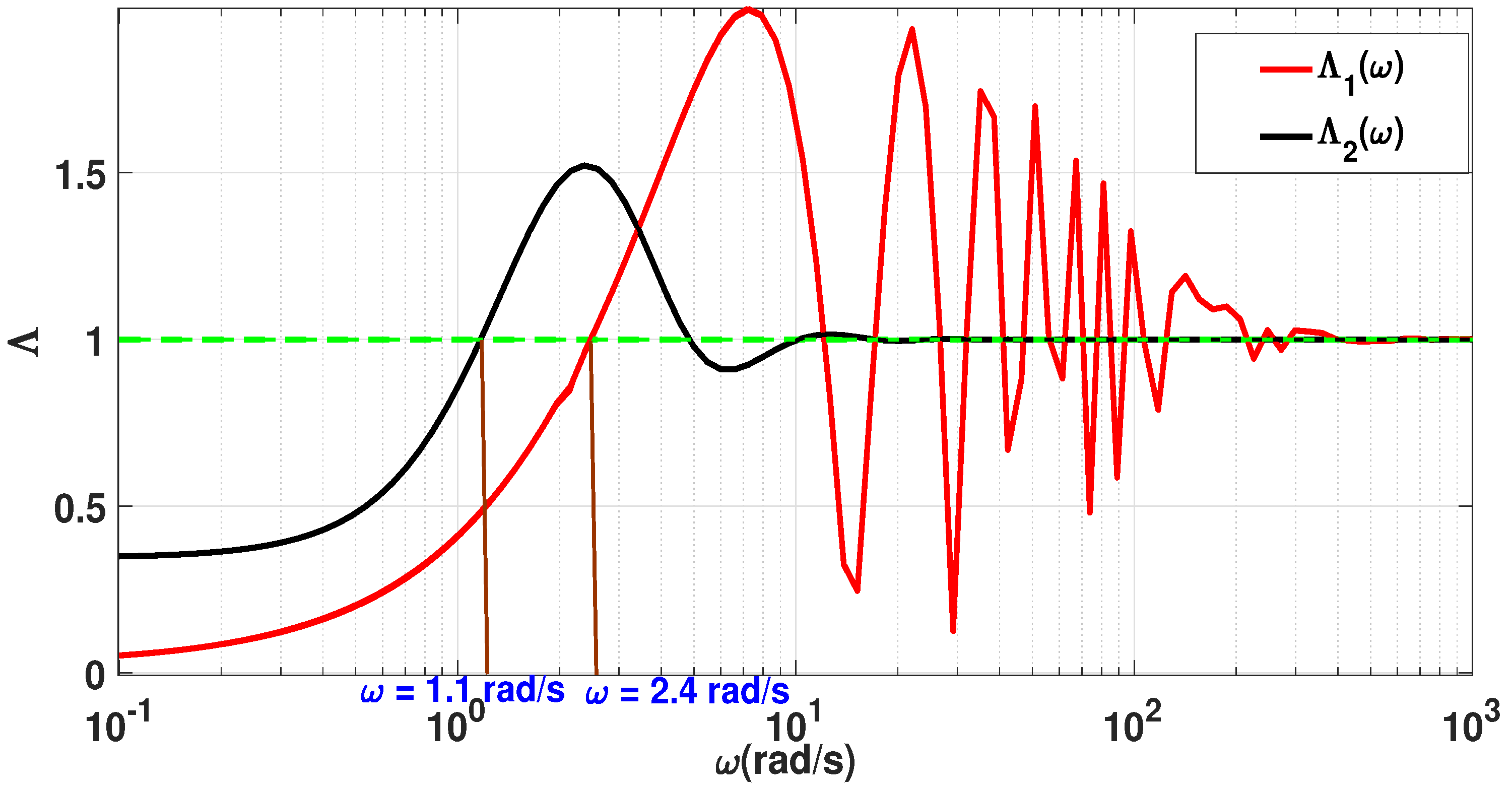
The values of ${\lambda }_{11}$ and ${\lambda }_{22}$ were tuned through simulation studies, with the aim of enhancing disturbance rejection performance while maintaining system stability. The selected values provided the best trade-off between response speed and robustness to external disturbances in both the vertical and horizontal channels. If the values of ${\lambda }_{11}$ and ${\lambda }_{22}$ are modified, it can impact the frequency range over which the disturbance rejection is optimized: (1) increasing $\lambda$ values can widen the effective disturbance rejection frequency range but may risk stability or increase sensitivity to noise, or (2) decreasing $\lambda$ values reduces disturbance rejection effectiveness, potentially narrowing the frequency range, but can improve the stability of the system.

Figure 3 plots ${\mathrm{\Lambda }}_1\left(\omega \right)$ and ${\mathrm{\Lambda }}_2\left(\omega \right)$. The green line represents the threshold line at ${\mathrm{\Lambda }}_k\left(\omega \right)=1$. This line serves as a reference: when ${\lambda }_k\left(\omega \right)<1$, $SP-H$ provides better disturbance rejection than $SP$; and when ${\lambda }_k\left(\omega \right)>1$, $SP$ performs better. The red curve corresponds to ${\mathrm{\Lambda }}_1\left(\omega \right)$, which evaluates the robustness function for the pitch angle $\psi$. The black curve corresponds to ${\mathrm{\Lambda }}_2\left(\omega \right)$, which evaluates the robustness function for the yaw angle $\varphi$.

The figure demonstrates that $SP-H$ rejects disturbance effects more effectively than $SP$ in the frequency range of $[0,1.1]$ rad/s for the pitch angle $\psi$, and in the range of $[0,2.4]$ rad/s for the yaw angle $\varphi$.

4. Simulation Results

To confirm the effectiveness of the proposed $SP-H$ controller, the linearized model of the feedback instrument $TRMS$ 33-220 was implemented in Simulink (Matlab). The step responses of this control scheme are presented in this section and compared to those of the conventional $SP$ controller, emphasizing both set-point tracking and disturbance rejection. Both $SP$ control schemes were applied to the linearized model of the $TRMS$ given in Equation (8). The amplitudes of the reference step inputs were set to $0.4$ rad for the vertical plane and $1.4$ rad for the horizontal plane. A step disturbance of $-0.3$ rad was introduced at 80 s to simulate an external perturbation.

In the control structure implemented in the simulation, the main controller parameters from Equation (21) were used to command the $TRMS$ system. Additionally, the decoupler parameters from Equation (9) were applied to separate the system into two subsystems: vertical and horizontal. Furthermore, the disturbance rejection controller parameters from Equation (41) were utilized to enhance the system’s performance.

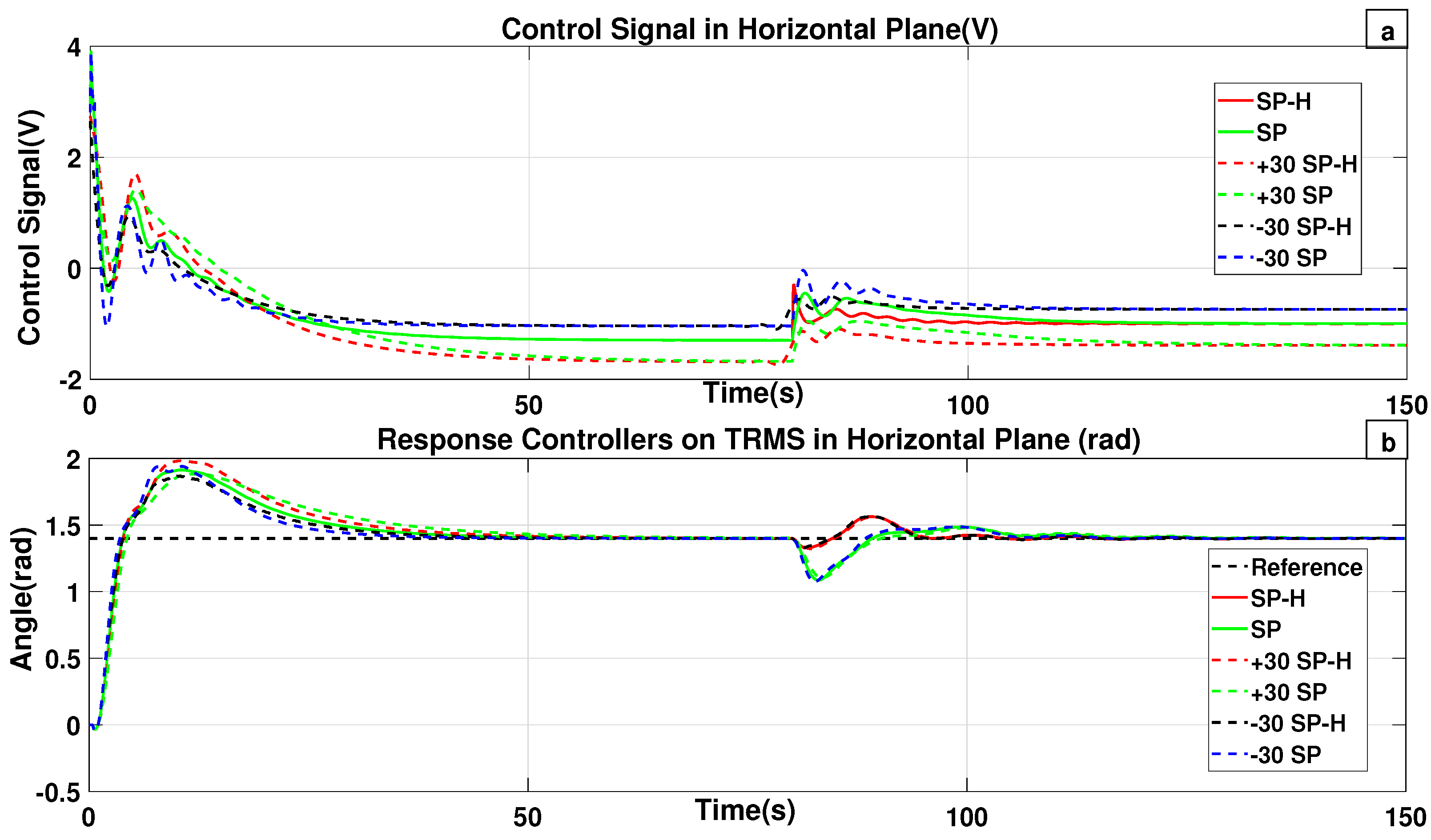
The responses of the control schemes applied to the $TRMS$ system in both the vertical and horizontal planes are illustrated in Figure 4 and Figure 5. Figure 4b presents the responses of both the $SP$ and $SP-H$ controllers on the vertical plane, while both controllers exhibit similar behavior in response to a reference change, they differ in their transient response when preventing external disturbances. Similarly, Figure 5b shows the responses of the same control schemes on the horizontal plane. Although the controllers demonstrate comparable behavior in terms of reference tracking, they display noticeable differences in transient performance during disturbance rejection. The control signals applied to the vertical and horizontal planes are displayed in Figure 4a and Figure 5a, respectively.

The classical $SP$ lacks a dedicated component for disturbance rejection; although it can attenuate disturbances, its response is slower compared to the proposed scheme. In the proposed $SP-H$ approach, the controller $H\left(s\right)$ significantly improves disturbance rejection capabilities. The simulation results outlined in Figure 4b and Figure 5b indicate that $SP-H$ exhibits superior disturbance rejection performance, providing improved transient behavior, in contrast to the conventional $SP$ scheme.

To evaluate the performance of our control system under varying operating conditions, we conducted simulations with $\pm 30\%$ variations in all $TRMS$ parameters, except for the time delay. The time delay was excluded because the $SP$ scheme is sensitive to mismatches in time delay. However, it can be estimated in real time, allowing the controller’s time delay parameter to be retuned dynamically (e.g., [36]). Figure 4 and Figure 5 present the simulation results, which demonstrate that (1) both $SP-H$ and $SP$ exhibit a wide range of stability robustness (tolerating more than $30\%$ parametric variation); (2) the time responses to step-point tracking and step disturbances of both control systems show relatively small variations despite the parameter changes; (3) $SP-H$ rejects disturbances significantly more effectively than $SP$; and (4) the time responses to step-point tracking and step disturbances of $SP-H$ are more robust than those of $SP$, as they remain more consistent under parameter variations. We note that the system responses deteriorate when parameter variations exceed $\pm 30\%$, and the system becomes unstable for variations around $\pm 50\%$.

Table 2. Performance comparison of controllers for horizontal and vertical planes in a simulation setting.

Controller	Vertical Plane			Horizontal Plane
	$\mathit{IAE}$	$\mathit{ISE}$	$\mathit{TV}$	$\mathit{IAE}$	$\mathit{ISE}$	$\mathit{TV}$
SP	1.124	0.057	2.646	2.274	0.2073	3.969
SP-H	0.6582	0.01	4.177	1.292	0.1055	4.794

provides a comparison of the time-domain responses of the $SP$ control structures from the simulation, focusing on disturbance rejection, considering the effect of airflow generated by a fan ventilator. In this table, $IAE$ refers to the Integral of the absolute error, defined as:

$${\int }_{80}^{\infty }\left|\left(r\right(t)-y(t\left)\right)\right|·dt$$

(42)

$ISE$ denotes the Integral of the squared error, given by:

$${\int }_{80}^{\infty }{(r\left(t\right)-y\left(t\right))}^2·dt$$

(43)

and $TV$ represents the total variation in the control signal, expressed as:

$${\int }_{80}^{\infty }\left|{\displaystyle \frac{du\left(t\right)}{dt}}\right|·dt.$$

(44)

The first two indexes reflect the system’s ability to reject disturbance effects, while the third quantifies the control effort required. In this context, it measures the variation in the control signal during the application of the airflow disturbance on the $TRMS$. This metric is associated with actuator wear (as well as that of other physical components), the magnitude of the control signal, and the potential for actuator saturation.

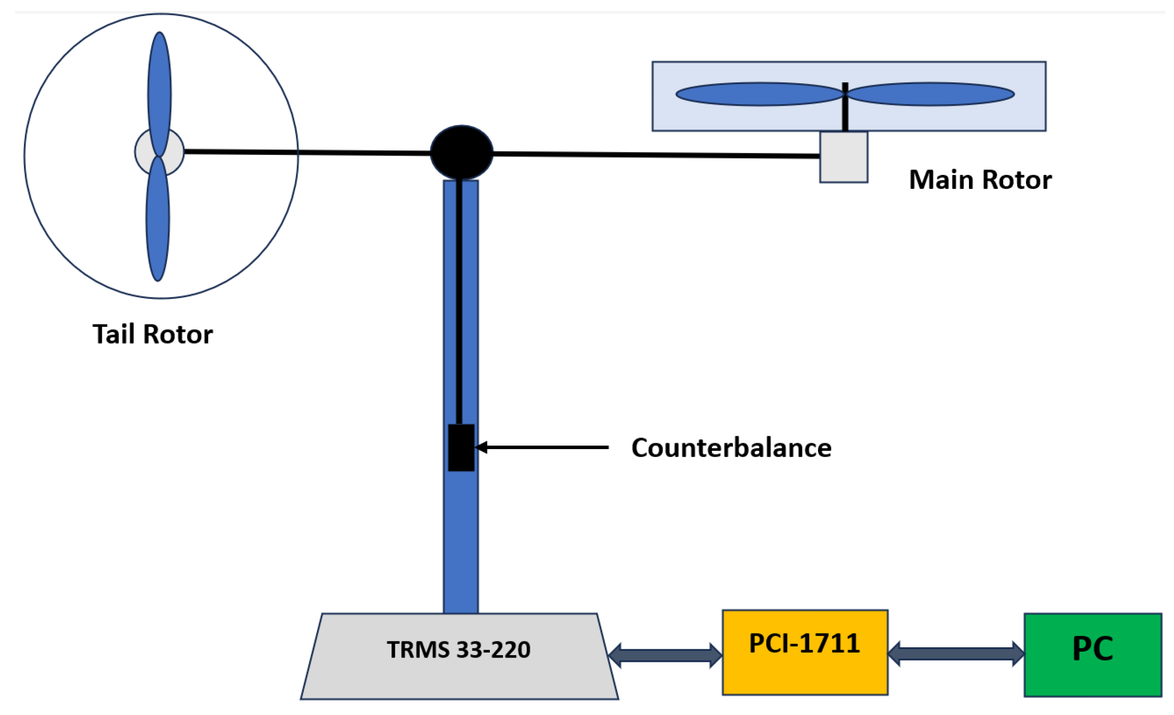
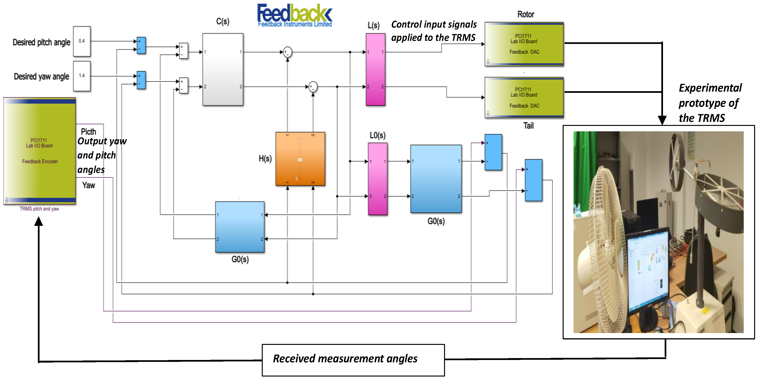
5. Experimental Results

To examine the practical effectiveness of the proposed controller, it was implemented into the $TRMS$ whose parameters are specified in Table 1. The $\left(PCI1711\right)$ laboratory unit is a feedback system consisting of two blocks: a feedback encoder block and a feedback $DAC$ block. The $TRMS$ uses two encoders to transmit the measurements of ($\psi$) and ($\varphi$) to the feedback encoder block. This block has three parameters: a sample time of $0.001$ $sec$, and offsets for channel one and channel two. Channel one corresponds to the first output of the encoder ($\psi$), while channel two corresponds to the second output of the encoder ($\varphi$). The value of the digital input provided to the $PCI1711$ is transformed into an analog response by the feedback $DAC$ block.

The proposed $SP$ control schemes were tested in real time by applying Simulink in Matlab on the actual $TRMS$ as shown in Figure 6. To demonstrate the performance of the proposed approach, experimental tests were conducted for the trajectory tracking problem of the $TRMS$. The experiments were conducted in a university laboratory under controlled conditions. The $TRMS$ setup, including the fan, data acquisition card, and computer, was placed on a stable table and isolated from external environmental disturbances. The main source of noise was the airflow generated by the fan, which was considered during testing.

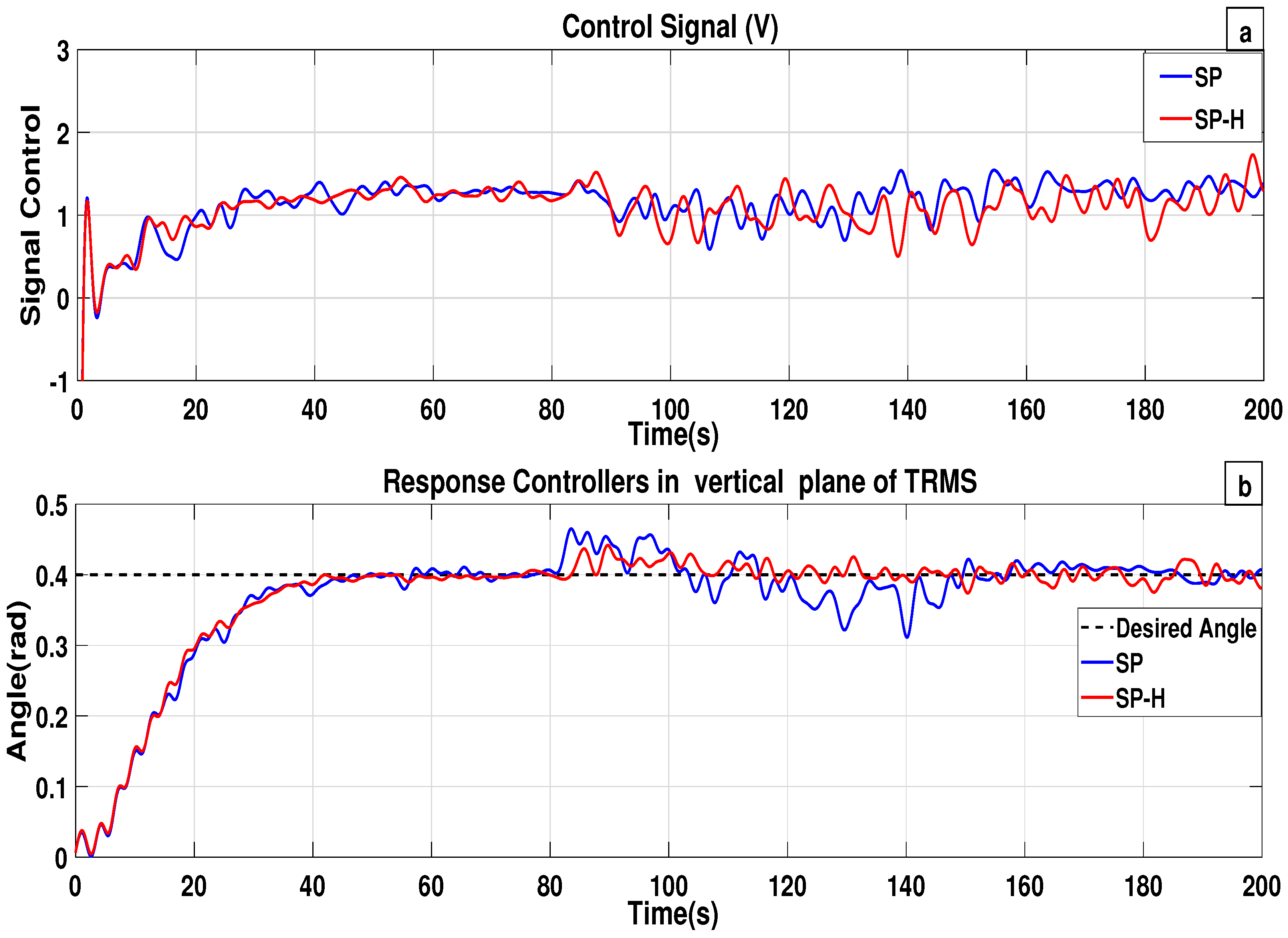
To evaluate the robustness of the proposed $SP-H$ control technique for rejecting external disturbances, a disturbance was introduced to the $TRMS$ at $t=80$ s. This disturbance consisted of an airstream generated by a Duracraft fan (240 V, 50 Hz, 50 W) placed approximately half a meter away from the system, directed at both the tail and main rotors. The airflow began approximately 80 s after the start of the experiment. The experiment results are shown in Figure 7 and Figure 8.

Figure 7b shows the performance of both controllers in controlling the vertical plane. It can be observed that while both controllers achieve satisfactory tracking of the reference signal, the $SP-H$ controller exhibits a superior transient response, particularly in the presence of external disturbances. The $SP-H$ controller reduces the overshoot and improves compared to the standard SP scheme, highlighting its robustness under real-world conditions. 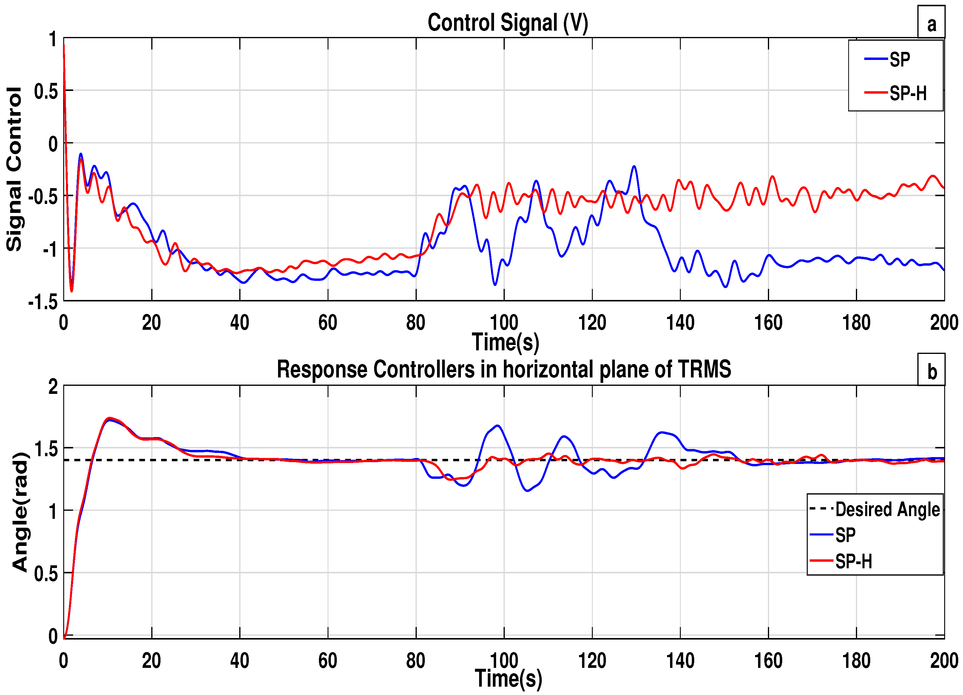Similarly, Figure 8b presents experimental outcomes for horizontal plane control. Both control schemes demonstrate effective reference tracking; however, the $SP-H$ controller shows enhanced disturbance rejection capabilities. During disturbance events, the $SP-H$ maintains a smoother and faster recovery, whereas the standard SP controller displays larger deviations. Figure 7a and Figure 8a illustrate the experimental control signals corresponding to the vertical and horizontal planes, respectively. These experimental findings confirm the improved performance of the proposed $SP-H$ method in practical scenarios, validating the advantages previously observed in simulation.

Table 3. Performance comparison of controllers for horizontal and vertical planes in an experimental environment.

Controller	Vertical Plane				Horizontal Plane
	$\mathit{IAE}$	$\mathit{ISE}$	$\mathit{TV}$	$\mathit{ME}$	$\mathit{IAE}$	$\mathit{ISE}$	$\mathit{TV}$	$\mathit{ME}$
SP	0.2825	0.0121	14.4361	0.1111	0.9497	0.1414	9.9422	0.2895
SP-H	0.1355	0.0024	13.9009	0.0618	0.3132	0.0220	15.2019	0.1547

presents a comparison of the time-domain responses of the $SP$ and $SP-H$ controllers based on experimental results when subjected to disturbances from the ventilator’s airflow. The maximum error $ME$ in this table is defined as $ma{x}_{t\in [80,\infty ]}\left|\left(r\right(t)-y(t\left)\right)\right|$, and the $IAE$, $ISE$ and $TV$ are also reanalyzed. It is observed that the $IAE$ and $ISE$ index values for the $SP-H$ controller are reduced compared to those of the $SP$ controller, although this improvement comes at the expense of an increase in control action. Moreover, the performance indices obtained from the experiments closely align with those from the simulations, validating the accuracy of our models and reinforcing the relevance of the comparative simulation analysis presented in the previous section.

6. Conclusions

This paper focuses on the mitigation of the airflow disturbance effects on the $TRMS$, with particular attention to reducing the impact of a fan ventilator. Due to the inherent time delay in the $TRMS$ dynamics, a control scheme based on the Smith predictor has been employed. Furthermore, a novel modification of the Smith predictor has been developed to enhance the control performance on the $TRMS$.

This research makes several key contributions, outlined as follows: (1) a multi-variable control method based on the Smith predictor controller capable of compensating for time delays and mitigating the effects of external disturbances while exhibiting good robustness features; (2) a novel methodology that adapts the $SP-H$ structure-originally developed in [31] for a second order plus time-delay system—to control higher-order time delay systems, specifically applied to the $TRMS$; (3) a comparative simulation analysis demonstrates that the proposed scheme achieves the same set-point tracking performance as the widely known $SP$ (for the nominal process) while greatly improving the attenuation of air disturbances caused by the fan; and (4) an experimental evaluation of this control scheme on a $TRMS$ prototype, confirming its superior performance compared to the standard $SP$. All comparisons were conducted fairly, using the same controller $C\left(s\right)$ in each case.

The $SP$ structure is highly sensitive to inaccuracies in the nominal time delay. This paper has not addressed the issue of varying time delays. However, this limitation can be mitigated by rapidly estimating the time delay in real time using algebraic identification techniques, which enables retuning of the internal model used in the $SP$. We refer to our recent work [36], where an adaptive $SP$ was designed and implemented on a teleoperated flexible-link robot with time-varying delay, based on real-time delay estimation using such an algebraic identification technique.

If the hardware-induced delay were known, it could be incorporated into the nominal model’s time delay and, consequently, into the $SP$ structure. If not, an identification method—such as the aforementioned algebraic identification technique—could be employed to estimate the delay in real time and retune the Smith predictor accordingly.

Our $SP-H$ eliminates steady-state errors caused by impulse or step-like disturbances. Since we are using linearized models, this property is validated independently of the disturbance amplitude. Such amplitude may introduce a steady-state error and/or alter the response shape only if it is large enough to drive the system dynamics outside the valid region of the linearization, or if it causes actuator saturation. It is worth noting, however, that ramp or parabolic-like disturbances would still result in steady-state errors. Even in these cases, our $SP-H$ enhances the disturbance rejection capabilities compared to the original $SP$.

The main contribution of this work is the enhancement of flight control for unmanned aerial vehicles ($UAV$s) of the helicopter type in the presence of strong air currents, thereby improving the system’s overall stability and performance. This advancement enables more precise and reliable operation, even under challenging environmental conditions.