A Novel Hybrid Deep Learning Model Enhanced with Explainable AI for Brain Tumor Multi-Classification from MRI Images

Abstract

The life span and quality of a patient are greatly diminished by a brain tumor, a type of cancer. For patients, early diagnosis and effective treatment are very significant in this respect. To assist medical professionals in this difficult and error-prone process and improve both the accuracy and interpretability of the model, this study proposes a new hybrid deep learning model enhanced with explainable artificial intelligence for brain tumor multi-classification from MRI images. It integrates a customized CNN model for feature extraction from images and the optimized XGBoost method with high classification success. It also incorporates Grad-CAM, which makes the black-box structure of the model transparent and the decision-making process more understandable. The proposed model classified four different brain tumors, namely glioma, meningioma, notumor and pituitary, with 99.77% accuracy and demonstrated superior performance when compared with existing methods. The results show that a robust, interpretable and high-performance hybrid classification model has been developed for brain tumor detection.

1. Introduction

Masses created by cells growing improperly in the brain are called brain tumors [1]. They occur in various sizes and shapes as benign and malignant. Benign tumors grow more slowly and cause less damage to brain tissues. Malignant tumors grow faster than benign ones and cause more damage, creating an extremely dangerous situation for human life. Although the cause of brain tumors is unknown, environmental and genetic factors, and some types of radiation, are effective in tumor formation. Along with these two forms of brain tumor, other common tumors are pituitary, glioma, and meningioma. A typically benign tumor called a meningioma forms on the brain and spinal cord’s meninges [2]. Surgery or radiation therapy can be used to treat this slow-growing tumor that gradually presses against the surrounding tissues. Pituitary tumors are often benign and arise from aberrant pituitary gland cell proliferation. Hormone deficits and visual issues may result from it [3]. The most prevalent malignant tumor is glioma. Approximately one-third of brain malignancies are caused by it. The prognosis for glioblastoma, the late stage of glioma, is dismal and ranges from one to one and a half years after diagnosis [4].

Benign or malignant tumors grow over time and create high pressure inside the skull. The brain tissues are damaged by this pressure effect. In order to minimize this damage and increase the patient’s survival rate, the brain tumor should be detected as early and accurately as possible. In addition to the expertise of radiologists, imaging techniques are also of great importance in tumor detection. There are modalities such as computed tomography (CT), positron emission tomography (PET), X-rays and magnetic resonance imaging (MRI) to diagnose brain tumors [5]. MRI is more useful than other methods and is one of the most efficient techniques to obtain detailed information about the anatomy, location, shape, and size of the tumor [6].

Brain tumors are a health problem with high mortality rates worldwide. Early detection of tumors, making the correct diagnosis and starting appropriate treatment as soon as possible are very important for the patient’s life expectancy and quality. Traditional methods used to diagnose brain tumors are based on manual examination of imaging data by radiologists. However, since these examinations depend on the expertise of the radiologist, they are open to error, require intensive labor and are time-consuming processes [7]. Performing such a process automatically and as quickly and accurately as possible will directly affect a patient’s life with the advantage of early diagnosis. The risk of spreading tumors that are detected at early stages can be prevented, the damage to brain tissues can be reduced and, since they may be smaller in size, they can be treated at a higher rate, with treatment methods such as radiotherapy, chemotherapy or surgical intervention. This reduces mortality rates and significantly improves patient life.

Machine learning (ML) and deep learning (DL) methods are utilized to automate the process of manually analyzing medical images. Machine learning methods use classified data. They classify new data of unknown class by learning features from labeled datasets. Classification can be undertaken on many datasets, including medical images, and using many methods [8], such as support vector machines (SVMs), k-nearest neighbor (KNN), naive Bayes (NB), decision tree (DT) and random forest (RF). Deep learning methods automatically extract complex features from larger data using artificial neural networks. Data are processed through many layers and classification is achieved with higher accuracy rates [9,10,11]. While ML and DL models have shown notable progress in the highly rapid and accurate detection of brain tumors [12], their black box nature creates a lack of confidence in the results. As the explanations for the models’ decisions are unclear, it is difficult for medical professionals to trust the classification outputs of the models. In these types of medical applications, where the results obtained will significantly affect the patient’s life, explainability and interpretability will increase the confidence in the correctness of the decision. ML and DL models are supported by explainable artificial intelligence (XAI), which reveals which features or which regions of the image are effective in the decision made regarding an image, and, thus, transparency and understandability of the decisions are ensured [13,14]. In this way, medical experts understand the reason for the decisions made. This enables the model to be used as an aid in making medical diagnoses with increased confidence in its results.

For classifying brain tumors, a novel hybrid model is proposed in this paper. The main contributions of this study are as follows:

• By fusing the strengths of deep learning models for feature extraction from images and machine learning for classification, a CNN + XGBoost hybrid model has been developed for multi-class brain tumor classification.
• The study incorporates XAI techniques to improve the interpretability of the results. This makes it possible to comprehend the decision-making process of the model in greater detail and offers insightful information about the variables affecting the classification results.
• A reliable and accurate model that can be used by medical professionals is provided, both by performing high-accuracy multi-classification and by providing visual reasons for the model outputs.
• A comprehensive evaluation showing the ability of the proposed model to effectively classify brain tumors and the interpretability of results through XAI is provided. This contributes to the growing medical image classification field by offering a robust and explainable model.

The paper is structured as follows. For classifying brain tumors, related work in the literature is presented in Section 2. Our proposed methodology, including the details of the CNN architecture, XGBoost algorithm, and Grad-CAM method is described in Section 3. Section 4 offers the results and its performance comparison with other models. Section 5 discusses the general conclusions of the paper.

2. Related Work

There are many studies that have performed binary and multiple classification of brain tumors using small or large datasets with machine learning and deep learning methods [15]. It is of great importance to perform brain tumor diagnosis automatically, quickly and accurately. Therefore, many methods have been proposed to increase accuracy and performance.

To classify brain tumors, a deep convolutional neural network architecture was proposed by Musallam et al. [16]. The quality of the used MRI images was enhanced by a three-step preprocessing technique, which produced a 97.72% classification accuracy for four distinct tumor types. Irsheidat et al. [17] developed a CNN model that used grayscale MRI input and expanded the dataset to fourteen times its original size. In test and validation data, the model’s accuracy in predicting the tumor or notumor was 88.25% and 96.7%, respectively. However, they only tested their model on a smaller dataset and performed a binary classification. A deep learning model for classification on datasets with different dimensions and modalities was presented by Sahu et al. [18]. This model uses an end-to-end cumulative learning strategy (CLS) and multi-weighted new loss (MWNL) function to reduce the effect of imbalance in the data and the overfitting problem with regularization functions such as DropOut and DropBlock. A modified RandAugment is proposed for the limited data problem and the classification success is increased with KNN. The proposed model outperforms other methods by reaching 99.7% accuracy when applied to small and imbalanced datasets. Sekhar et al. [19] proposed a model performing feature extraction with pre-trained GoogleNet and classification with SVM and KNN. Compared with other models, this model had the highest value accuracy for classifying a 3-class brain tumor using the CE-MRI Figshare repository and the Harvard Medical Archives. Khairandish et al. [20] proposed a hybrid model that classifies brain tumors as either benign or malignant by integrating CNN and SVM methods. In the study performed using a BRATS dataset, images were normalized, important features were selected utilizing a maximally stable extremal regions method and segmentation was performed. Following that, the CNN + SVM hybrid model classified the images with 98.4% accuracy.

Recently, XAI methods have become increasingly used to explain model decisions due to the lack of interpretability and understandability of the outputs obtained from DL and ML approaches [21]. Gaur et al. [22] proposed a dual-input CNN approach integrating SHAP and LIME methods to improve the model’s interpretability and classify brain tumors using MRI images. Utilizing a dual-input CNN model, robustness against noise and metal artifacts in image quality was ensured and brain tumors were multi-classified with a 94.64% accuracy rate by managing with low-quality images. Ten distinct transfer learning models were compared with regard to brain tumor classification performance by Nhlapho et al. [23]. The top-performing models were identified as EfficientNetB0, DenseNet121, and Xception, while the models’ outputs were interpreted using Grad-CAM++ and Grad-CAM. It was shown that transfer learning models provide a more efficient training process with the available data and provide high accuracy classification success. A three-stage method for brain tumor segmentation and classification was proposed by Saeed et al. [24]. The DeepLabV3+ model was used for segmentation in the first phase. Images were classed in the second phase after characteristics were retrieved using the Darknet53 and MobileNetV2 models and fed into the SVM model. In both the first and second stages, hyperparameters were tuned with Bayesian optimization. In the last stage, the decisions of the model were explained with XAI techniques. A 98% accuracy rate was achieved for segmentation and 97% for classification.

Upon reviewing the literature, it was discovered that the studies were limited to small datasets, accuracy rate was low, the classification was made as tumor or notumor instead of multiple classification, and that the proposed approaches were not supported by explainable artificial intelligence methods to ensure their reliability. For this purpose, the proposed study developed a model that classifies a large dataset containing MRI scans for four different tumor types, and the transparency of the model was provided by visualizing which region in the image the model’s prediction was focused on with XAI. Furthermore, a hybrid model was proposed that combines the strengths of both ML and DL.

3. Materials and Methods

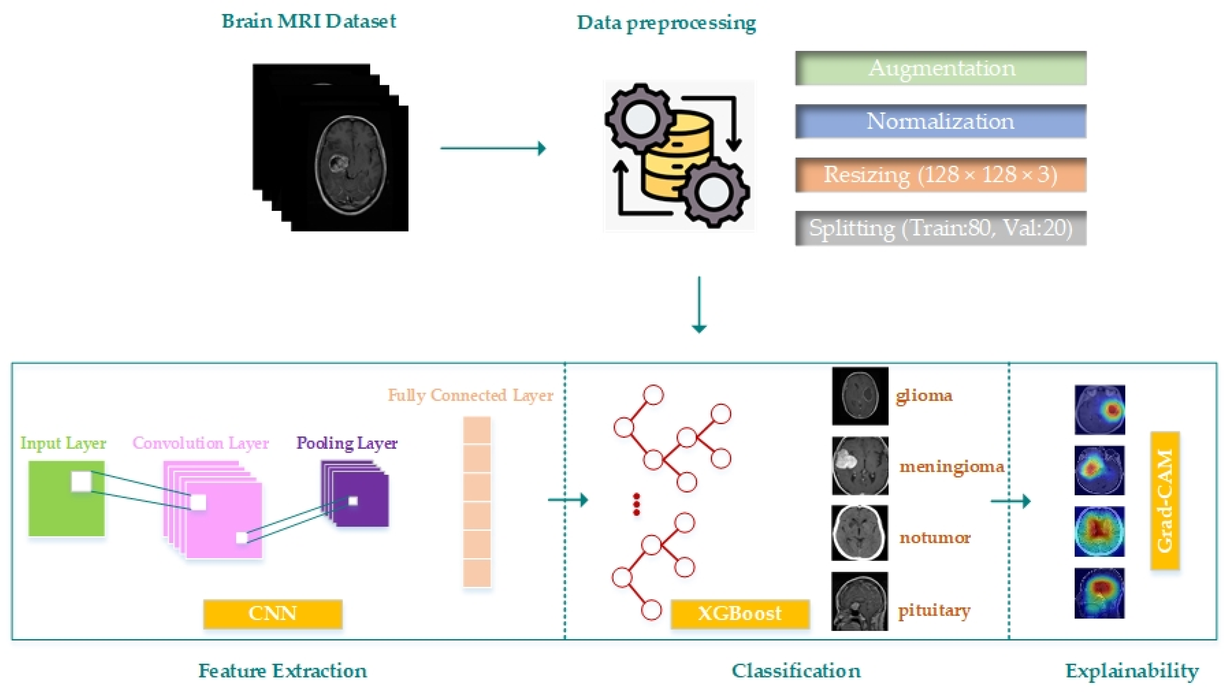
This paper proposes a hybrid model by developing a CNN model for brain tumor multiple classification and combining it with the XGBoost method. In addition, the result generation process of the model is made more clear and transparent with the integration of Grad-CAM. The proposed model’s block diagram is displayed in Figure 1. A process consisting of data preparation, augmentation and preprocessing, building the CNN model and feature extraction, classification of the extracted features with XGBoost and explanation of the classification decisions with Grad-CAM is proposed.

3.1. Dataset and Preprocessing

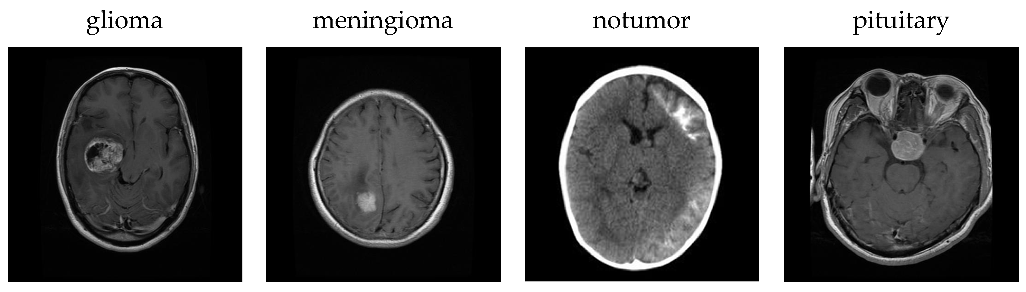
In this study, a publicly accessible dataset was acquired from kaggle.com by merging images from the Br35H, SARTAJ, and figshare datasets [25]. Each image is a 512 × 512 jpeg file. The dataset includes MRI scans of glioma, meningioma, notumor and pituitary brain tumor types. The dataset contains 7023 images in total, consisting of 1311 test data and 5712 training data. The number of training and test MRI images for each class is detailed in

Table 1. Dataset summary.

Tumor Type	Training	Testing
Glioma	1321	300
Meningioma	1339	306
Notumor	1595	405
Pituitary	1457	300
Total	5712	1311

. Figure 2 shows sample images for each class in the dataset.

Before using the dataset to train the CNN model, data augmentation and preprocessing steps were applied. First, the TensorFlow/Keras library’s ImageDataGenerator class was used to apply a variety of data augmentation techniques to the training data. Images were zoomed (zoom_range = 0.2), rotated at random angles (rotation_range = 20), horizontally flipped (horizontal_flip = True), shifted (shear_range = 0.2) and vertically and horizontally shifted (height_shift_range = 0.2, width_shift_range = 0.2) with the given parameter values. With the fill_mode = ’nearest’ parameter, newly formed pixels were filled with the value of their nearest neighbors. In this manner, the diversity of the training data was expanded, it was ensured that more images were used for training and the model’s generalization ability was strengthened. No augmentation process was applied for the test data. Then, preprocessing steps were applied to provide better performance by making both the training and test data suitable for the model. Resizing the images (128 × 128), transforming grayscale images to RGB images (128 × 128 × 3), and normalizing the pixel values to the range of 0–1, are the preprocessing techniques used. Lastly, 20% and 80% of the dataset, respectively, are divided for validation and training.

3.2. Proposed Model

The proposed hybrid model is a three-stage process: feature extraction with a customized CNN model, classification with XGBoost, and explainability of classification predictions with Grad-CAM.

3.2.1. Feature Extraction

Features are extracted with the developed CNN architecture and images are classified based on these features with XGBoost. For this purpose, the last dense layer of the CNN architecture that performs classification is removed and the features obtained from other layers are given to XGBoost as input. The classification success depends on the features extracted from the CNN model. Therefore, a CNN model that extracts features in a way that provides high classification accuracy has been developed. To understand the contribution of replacing the CNN’s fully connected layer with XGBoost, an ablation study was conducted. According to the results of the ablation study, when only CNN was used, the model achieved 97.80% accuracy. When the fully connected layer and XGBoost were added to CNN, the accuracy increased to 98.73%. However, the highest accuracy value of 99.77% was obtained from the model where only CNN and XGBoost were used together. The results show that the highest performance is achieved with the proposed system architecture and that high-level semantic information is preserved and further utilized effectively. Although the performance of the CNN model is improved by stacking the fully connected layer outputs with XGBoost, the most successful results are obtained with the proposed model.

In Figure 3, the proposed CNN model architecture is displayed. The model consists of three convolution layers (Conv2D) with 32, 64 and 128 filters. Each layer uses a 3 × 3 kernel size and the ReLU activation function. While lower-level feature information is extracted with the first convolution layer, more complex patterns and features are extracted with the following convolution layers. After each convolution layer, 2 × 2 MaxPooling is implemented to decrease the computational load by reducing the feature maps’ dimensions and to increase the model’s ability for generalization. The risk of overfitting is reduced by applying a 0.3 dropout after convolution layers and a 0.5 dropout after fully connected layers. The multidimensional feature maps created by the convolution layers are converted to a one-dimensional vector with the flatten layer and transferred to fully connected layers (dense layers). These layers employ the ReLU activation function and have 256 and 128 neurons. The model can compute probabilities between four classes thanks to the last layer’s 4-neuron output layer with a softmax activation function. However, this last layer was removed when combining with XGBoost.

The CNN model is trained using certain parameters.

Table 2. Hyperparameter values of CNN model.

Hyperparameter	Value
Optimizer algorithm	Adam
Batch_size	32
Epoch	50
Loss function	Cross-Entropy

lists these parameter values. The Adam algorithm was used for model optimization, and categorical cross-entropy, which works well for classification into several classes, was used as the loss function. Training was performed with 32 batch_size and 50 epochs. The model consists of 6,548,868 parameters.

3.2.2. Classification

Recently, hybrid models have been developed by combining DL and ML methods to increase the classification success [19,26,27]. Deep learning methods have strong representation capabilities. Gradient boosting methods provide high accuracy in classification. Therefore, a hybrid model that combines XGBoost with the customized CNN model is proposed in this study. High-level features are extracted from images with CNN, and classified with high accuracy and speed with XGBoost. The overall performance is increased by classifying with XGBoost instead of CNN’s fully connected layer and softmax classifier.

XGBoost, proposed by Tianqi Chen and Carlos Guestrin [28], is created by optimizing the gradient boosting algorithm. Its most important features are high accuracy, preventing overfitting, handling empty data and speed. It uses gradient boosting decision trees as weak learners. The model works iteratively and each tree generates a new model by correcting the errors in the previous trees [29]. Error rates are reduced by using gradient descent. The goal is to minimize the loss L between the true value y and $\hat{\mathrm{y}}$ given a prediction model f(x). The loss is stated by Equation (1).

$$\mathrm{L}=\sum {\left({\mathrm{y}}_{\mathrm{i}}-{\hat{\mathrm{y}}}_{\mathrm{i}}\right)}^2$$

(1)

XGBoost uses number of trees (n_estimators), learning rate (learning_rate) and tree depth (max_depth) parameters and the performance is highly dependent on these parameter values. Therefore, GridSearchCV method is used to determine the correct parameter values. GridSearchCV is a brute force approach that optimizes the hyperparameters of machine learning approaches and tries all combinations for the hyperparameter ranges specified by the users. The performance is calculated for each hyperparameter combination and the best hyperparameter set is selected. The best parameter values for XGBoost optimized with GridSearchCV are given in

Table 3. Hyperparameter values of XGBoost.

Hyperparameter	Value
n_estimators	100
learning_rate	0.01
max_depth	3

.

3.2.3. Explainability

The outputs of classification models created based on DL or ML techniques are not transparent enough to clearly show the reasons for model decisions. Therefore, the comprehensibility and interpretation of the obtained results becomes difficult. In this case, it is not reliable for experts to act according to a decision without knowing the reason for this decision [30]. XAI methods that make the internal workings and decision process of the model understandable in a way that increases this level of confidence have recently been integrated into models and more transparent outputs are offered [31]. XAI explanations are performed at different levels: global, local and semi-local. Global explanations provide an explanation of the general behavior of the model. They provide an understanding of the model’s output distribution and help one to understand how it works in general. They do not provide an explanation based on single samples. Local explanations provide explanations for specific input samples. The reason for the decision made for a sample is explained. Semi-local explanations provide local explanations for a group of data consisting of similar samples.

Grad-CAM is an XAI method that visualizes the results of deep learning models and makes model decisions explainable [31]. A more transparent result is provided by utilizing the power of visualization techniques to determine which regions of medical images, such as X-rays and MRI, the model focuses on [32]. In a classification problem, the regions that are effective in assigning the class of the image are visualized using heat maps. As the class output of a model is obtained from the last layers, Grad-CAM is applied to these last layers. Gradients containing information about the model’s class predictions are obtained. These gradients are multiplied with the feature maps in each layer. This weighted average shows which regions affect the model decision more for each class. The resulting weighted feature maps are converted into heat maps. On these maps, cold colors show regions that are less considered by the model, while warm colors show regions that are more considered. Thus, it is clearly shown which regions on the image are effective in creating the class label. This enhances understanding of how the model makes decisions.

3.3. Performance Evaluation

The performance of classification models is determined using different metrics. These metrics are intended to assess how well the classifier uses both the predicted and actual class values. Among these, F1 score, precision, recall and accuracy are the most frequently utilized. The calculation of these metrics is performed using the confusion matrix. The confusion matrix compares the values predicted by a classification model with its actual values. This matrix is created using true positives ${(\mathrm{T}}_{\mathrm{P}})$, true negatives ${(\mathrm{T}}_{\mathrm{N}})$, false positives ${(\mathrm{F}}_{\mathrm{P}})$ and false negatives ${(\mathrm{F}}_{\mathrm{N}})$. Thanks to this matrix, the prediction success of the classification model according to different classes is obtained by calculating the precision, recall, F1 score and accuracy metrics. Accuracy is defined via Equation (2) as the percentage of samples accurately predicted by the model.

$$\mathrm{Accuracy}={\displaystyle \frac{{\mathrm{T}}_{\mathrm{P}}{+\mathrm{T}}_{\mathrm{N}}}{{\mathrm{T}}_{\mathrm{P}}{+\mathrm{T}}_{\mathrm{N}}{+\mathrm{F}}_{\mathrm{P} }{+\mathrm{F}}_{\mathrm{N}}}}$$

(2)

Precision indicates the proportion of samples that are genuinely positive and is measured via Equation (3).

$$\mathrm{Precision}={\displaystyle \frac{{\mathrm{T}}_{\mathrm{P}}}{{\mathrm{T}}_{\mathrm{P}}{+\mathrm{F}}_{\mathrm{P}}}}$$

(3)

Recall demonstrates the proportion of actual positive samples that are correctly predicted and is calculated via Equation (4).

$$\mathrm{Recall}={\displaystyle \frac{{\mathrm{T}}_{\mathrm{P}}}{{\mathrm{T}}_{\mathrm{P}}{+\mathrm{F}}_{\mathrm{N}}}}$$

(4)

The harmonic average of the precision and recall scores is denoted as the F1 score and is defined via Equation (5).

$$\mathrm{F}1\text{-}\mathrm{score}=2 \times {\displaystyle \frac{\mathrm{Precision} \times \mathrm{Recall}}{\mathrm{Precison}+\mathrm{Recall}}}$$

(5)

3.4. Experimental Setup

All experiments for this study were performed using Python 3.12 on a computer with 12 GB of RAM, a 256 GB SSD, a 64-bit operating system, a 2.60 GHz Intel Core i7-6700HQ CPU and a NVIDIA GeForce 950M. Tensorflow, scikit-learn, os, matplotlib, cv2, numpy, and the seaborn libraries were used for dataset preprocessing and augmentation, model creation and analysis of the results.

4. Results and Discussion

The CNN + XGBoost model performance in the multiple classification of brain tumors will be presented in this section. The contribution of model decision explanations to the classification process by adding the Grad-CAM method will be discussed. Additionally, the efficacy of the model will be assessed by comparing the outcomes with other machine learning methods, pre-trained models and state-of-the-art methods. Additionally, the efficacy of the model is assessed by comparing the outcomes with other machine learning methods, pre-trained models and state-of-the-art methods, all tested under the same experimental conditions. All models were trained and evaluated using the same dataset, feature sets, preprocessing steps, and data split ratios to ensure consistency and fairness in comparison.

Four different brain tumors were classified by the CNN + XGBoost model as pituitary, meningioma, glioma, and notumor. The confusion matrix for classification results is displayed in Figure 4. The matrix shows that the model generally predicts classes with high accuracy rates. The model incorrectly identified 1 out of 300 images as meningioma in the glioma class, whereas it correctly identified 2 out of 306 images as gliomas in the meningioma class. Such a result depends on the classification ability of the model as well as the medical characteristics of the tumors. Although glioma and meningioma tumors originate from different cell types, in some cases their morphological characteristics may be similar. Large and invasive meningioma can be confused with gliomas. Such meningioma can spread to deeper areas of the brain and show similar characteristics to gliomas as they come into contact with the meninges. Therefore, it becomes difficult to distinguish them from gliomas. While gliomas have a rapidly growing irregular structure, meningioma grow slowly and affect a limited area. However, some can grow rapidly and show similar invasive characteristics to gliomas. As a result, it becomes difficult to distinguish such tumors for the model. Every image in the other two classes was appropriately classified. A model with a very low rate of misclassification and a high rate of class separation was produced when a general analysis is performed on the precision, recall, and F1 score values for each class shown in

Table 4. CNN + XGBoost model classification results.

Tumor Class	Precision	Recall	F1 Score
Glioma	0.993	0.997	0.995
Meningioma	0.998	0.993	0.995
Notumor	1.0	1.0	1.0
Pituitary	1.0	1.0	1.0

.

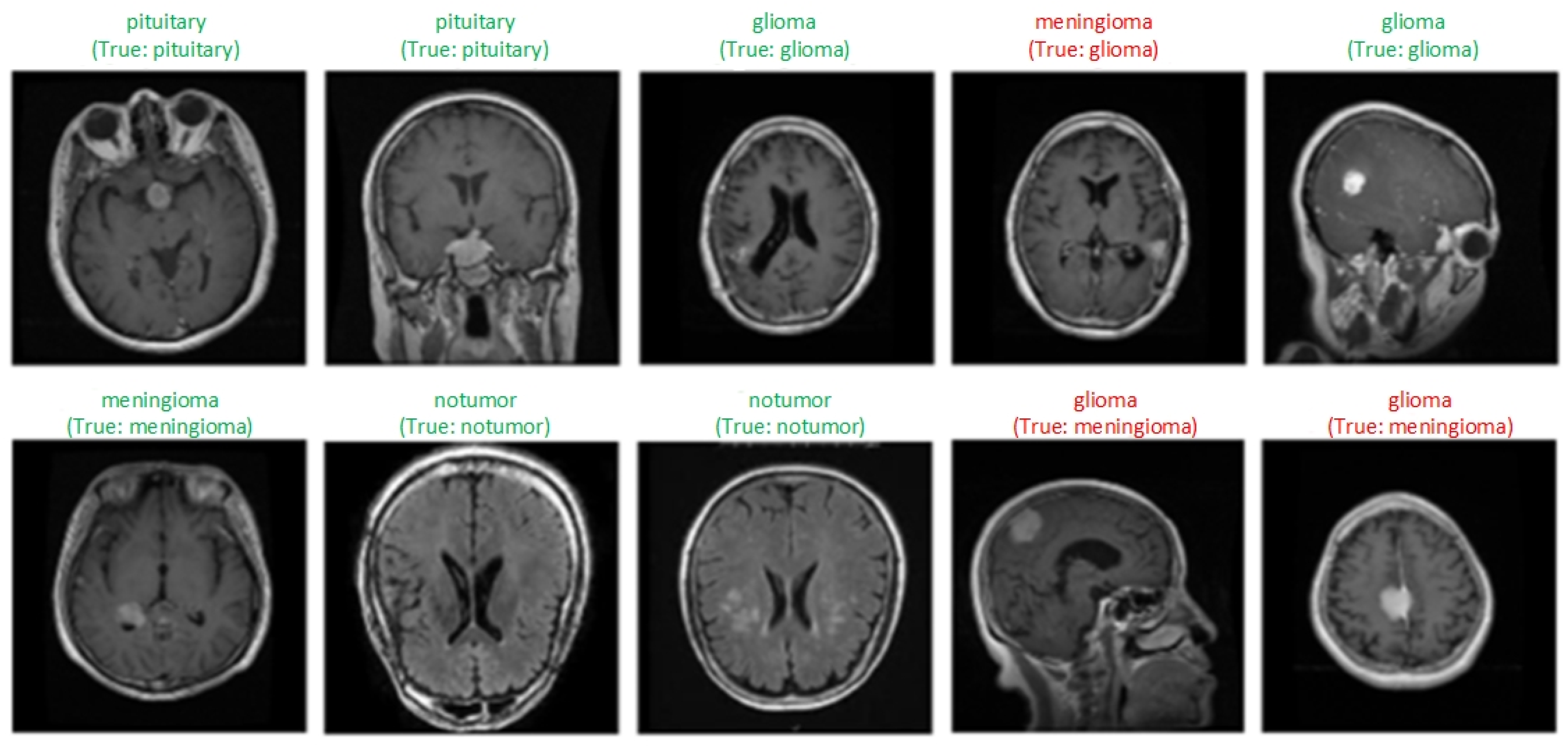
Figure 5 shows samples of each class obtained as a result of the classification of MRI scans by the model. Labels expressed as “True” indicate the actual class of the image, and the one above shows the class label predicted by the model. Green labels show correctly classified samples, and red labels indicate incorrectly classified samples. Three samples whose classes were incorrectly predicted by the model and some correctly classified samples are visualized. The model generally classified the images correctly. Misclassifications may be due to the similar structural features of tumors.

In Figure 6a, each column shows three original MRI images and the class labels predicted by the model for the classes glioma, meningioma, notumor and pituitary, respectively. In (b), the regions that the model takes into consideration when assigning this class label are visualized with Grad-CAM. In the generated heat maps, red and yellow colors indicate the most important regions, while blue and green colors indicate less important regions. In the glioma image, the tumor is usually located in the deep cerebral regions, and this region is clearly highlighted in red on the Grad-CAM maps. This shows that the model can correctly identify the tumor area. In the meningioma image, the model correctly detected the location of the tumor near the dura mater and the activation maps generally showed high focus around the lesion. In the notumor image, the model focused on a wider area and could not highlight a distinct region because there was no tumor. In the pituitary image, the activation of the model was concentrated in the region where the pituitary gland is located, indicating that even small and deep-seated tumors can be successfully localized. These visualizations clearly revealed the regions that should be focused on in the image for each tumor type and that the model not only achieves classification success but also makes decisions by taking into account medically meaningful regions, significantly increasing the interpretability of the model.

To verify the generalizability of the proposed model, multiple brain tumor classification was performed using a publicly available dataset obtained from kaggle.com, one which was not used in the training or validation stages of the model. By selecting 500 images for each class from this dataset, a balanced distribution was created to eliminate overfitting due to class imbalance. Figure 7 shows the classification results of the proposed model for the external dataset. As can be seen, the model classified the notumor class without error and the number of incorrectly classified images in other classes was low.

Table 5. CNN + XGBoost model classification results for the external dataset.

Tumor Class	Precision	Recall	F1 Score
Glioma	0.997	0.982	0.990
Meningioma	0.970	0.988	0.979
Notumor	0.994	1.0	0.997
Pituitary	0.994	0.986	0.990

shows the precision, recall and F1 score values for each class. The model achieved 98.90% accuracy on the external dataset. Although slightly lower than the performance on the original test set, these results support the generalizability of the model.

4.1. Comparison with Machine Learning Methods

There are many machine learning approaches used to classify various data. SVM, KNN, DT, NB, RF and CatBoost are the most commonly used methods. These methods classify data using different parameters, and these values directly affect the classification success. Therefore, the hyperparameter values were optimized with GridSearchCV and the best values are given in the

Table 6. Parameters used for machine learning methods.

Method	Parameters
DT	min_samples_split: 2, criterion: entropy, min_samples_leaf: 1, max_depth: 20
KNN	algorithm: auto, metric: minkowski, n_neighbors: 3
SVM	gamma: scale, C: 0.1, kernel: linear
RF	max_depth: None, n_estimators: 50

. A more generalizable SVM model was obtained by using a linear kernel and a low C value. In the classification with KNN, the algorithm automatically selects the most appropriate method with three neighbors and the Minkowski distance metric. For DT, the risk of overfitting was reduced by selecting information gain-based division (entropy) and a maximum depth of 20. For RF, 50 trees were used without being restricted by the maximum depth. The CatBoost model was configured with a small learning rate (0.01) and 100 iterations, providing a balanced learning process. To improve the models’ accuracy and generalization performance, these parameters were chosen through GridSearchCV optimization.

To assess the consistency and robustness of the proposed CNN + ML hybrid models, the standard deviations of classification accuracy over 10 independent runs were calculated for each model. In each run, the dataset remained constant, while the training and test data were resplit by 80–20% with different random selections. During these processes, the features extracted from the CNN model for each run were classified with machine learning methods and the accuracy value was calculated. The standard deviation was calculated over the 10 accuracy scores obtained. In

Table 7. Accuracy standard deviations of CNN + ML models.

Model	Std
CNN + SVM	0.0168
CNN + KNN	0.0150
CNN + DT	0.0066
CNN + NB	0.0167
CNN + RF	0.0262
CNN + CatBoost	0.0165
CNN + XGBoost	0.0025

, the results indicate that the CNN + XGBoost model not only achieved the highest mean accuracy but also exhibited the lowest standard deviation, with 0.0025, demonstrating superior stability across different runs. In contrast, the CNN + RF model showed the highest standard deviation, with 0.0262, suggesting a higher sensitivity to data partitioning or initialization.

Table 8. Classification performance comparison of CNN + ML models.

Model	Class Type	Precision	Recall	F1 Score	Accuracy (%)
CNN + SVM	G	0.986	0.950	0.967	98.03
	M	0.951	0.967	0.959
	N	0.992	1.0	0.996
	P	0.987	0.996	0.991
CNN + KNN	G	0.982	0.953	0.967	97.95
	M	0.954	0.964	0.959
	N	0.992	1.0	0.996
	P	0.983	0.993	0.988
CNN + DT	G	0.993	0.983	0.988	99.16
	M	0.980	0.983	0.982
	N	1.0	1.0	1.0
	P	0.990	0.996	0.993
CNN + NB	G	0.982	0.950	0.966	97.80
	M	0.951	0.957	0.954
	N	0.992	1.0	0.996
	P	0.980	0.996	0.988
CNN + RF	G	0.955	0.933	0.944	95.66
	M	0.903	0.933	0.918
	N	0.987	0.969	0.978
	P	0.976	0.988	0.982
CNN + CatBoost	G	0.979	0.950	0.964	97.86
	M	0.948	0.964	0.956
	N	0.992	1.0	0.996
	P	0.986	0.990	0.988
CNN + XGBoost	G	0.993	0.997	0.995	99.77
	M	0.998	0.993	0.995
	N	1.0	1.0	1.0
	P	1.0	1.0	1.0

compares the proposed CNN + XGBoost model’s performance values with machine learning techniques for the glioma (G), meningioma (M), tumor (N), and pituitary (P) classes. According to the results, the use of different ML algorithms together with CNN causes different performance results in brain tumor classification. The CNN + XGBoost model has the highest accuracy rate with 99.77% and very high precision, recall and F1 score values were obtained in all classes. All of the samples in two classes were classified correctly. The CNN + DT model ranked second with 99.16% accuracy rate, while other models exhibited similar performance in the range of 97.8–98.0% accuracy. The CNN + RF model has the lowest accuracy rate with 95.66%. These results demonstrate that the features extracted by CNN are processed most effectively thanks to the powerful classification capabilities of XGBoost. The proposed model classified multiple brain tumors more successfully when compared with other machine learning methods. The confusion matrices of all models are given in Figure 8. The number of correct and incorrect classifications for all classes can be seen more clearly from these matrices. These machine learning methods and XGBoost were combined with the developed CNN model and their classification success was compared. The results show that the XGBoost method classified images with higher accuracy based on the features extracted by CNN when compared with these methods.

4.2. Comparison with Pre-Trained Models

Transfer learning models are frequently used in brain tumor classification [33,34,35]. Thanks to the use of these models, training time is accelerated and the performance of the model is increased by using pre-trained neural networks. Instead of training a model with large datasets, it is sufficient to retrain only the last layers in pre-trained models. In addition, visual features are well learned and images are classified more successfully with these features. In this study, DenseNet121, ResNet50, EfficientNetB5, VGG19, Xception, InceptionV3 and MobileNetV2 from pre-trained models were used for performance comparison.

For the training and validation processes of the proposed model and pre-trained models, Figure 9 and Figure 10 show the accuracy and loss values, respectively. Although VGG19 is stable in training accuracy and loss, there are significant fluctuations in validation accuracy and loss. This shows that the model overfits the data and has difficulty in generalizing to new data. Although the other models have occasional fluctuations in terms of accuracy and loss, they appear to be models that give balanced results. The proposed model’s training and validation loss decreases in parallel, and its training and validation accuracies almost overlap. This shows that the model is resistant to overfitting and has a better generalization performance. As a result, the proposed model stands out as the model that performs better than other models, with small difference between the training and validation curves, a continuous decrease in loss values and high accuracy rates.

The pre-trained models’ confusion matrices are shown in Figure 11 and the test accuracy and loss values of these models are shown in

Table 9. Test accuracy and loss values of pre-trained models.

Model	Accuracy	Loss
DenseNet121	0.983	0.036
ResNet50	0.963	0.010
EfficientNetB5	0.974	0.090
VGG19	0.927	0.196
Xception	0.981	0.086
InceptionV3	0.985	0.048
MobileNetV2	0.961	0.247
Proposed model	0.997	0.005

. It misclassified only three samples and showed a more successful performance than all of the other models, with a 99.77% accuracy rate. It was by far the most successful model, achieving the highest accuracy and lowest loss value. InceptionV3 and DenseNet121 achieved the closest results to the proposed model by exhibiting high performance, with 98.5% and 98.3% accuracy rates, respectively. Xception (98.1% accuracy, 0.086 loss) and EfficientNetB5 (97.4% accuracy, 0.090 loss) models have lower performance due to their slightly higher loss values. ResNet50 is less successful than the other models with a 96.3% accuracy rate. VGG19 (92.7% accuracy, 0.196 loss) and MobileNetV2 (96.1% accuracy, 0.247 loss) are models with the lowest accuracy and high loss values, and have lower performance when compared with the others. Overall, the proposed model minimizes misclassifications for four tumor types and gives more successful results. The features extracted by a customized CNN structure were combined with a powerful machine learning algorithm such as XGBoost to provide higher classification accuracy. CNN is quite effective in extracting low- and high-level features from images, but in some cases it may have difficulty with more complex data. XGBoost, on the other hand, can perform more accurate and faster classifications using tree-based structures, especially in cases where the number of features is large and there are complex data relationships. The combination of CNN + XGBoost combines the advantages of both models. While CNN extracts high quality features, XGBoost evaluates the importance of these features and optimizes the classification process. In addition, as the size of the dataset used in the study is relatively small, pre-trained models carry the risk of over-training. These models are powerful in terms of learning complex features using very deep networks; however, they are more expensive in terms of computation and require very large data. They can be effective especially in very large datasets, but when working with limited data, difficulties such as slow learning and learning unnecessary features may be encountered. Experimentally, the proposed CNN + XGBoost structure has given higher accuracy results than these models based on transfer learning.

4.3. Comparison with State-of-the-Art Methods

Demonstrating the model performance against the best available approaches is essential for performance evaluation. In classifying brain tumors, the performance of the proposed model is highlighted by a comparison with state-of-the-art methods. Such a comparison helps to determine whether the model is superior in critical aspects such as accuracy and explainability. The architectures of the models, the type of classification, the visualization of decisions with explainability method, and the accuracy rate are the criteria taken into consideration for comparing the CNN + XGBoost model with the state-of-the-art methods.

Table 10. Comparison with state-of-the-art methods.

Reference	Class Type	Model	XAI	Accuracy (%)
[36]	Multi	SVM	No	96.67
[34]	Multi	InceptionV3	No	97.12
[37]	Binary	DenseNet121	No	97.86
[38]	Binary	CNN	No	98.82
[39]	Binary	CNN	No	98.50
[40]	Binary	VGG16	LRP	97.33
[41]	Multi	NeroNet19	LIME	99.30
[42]	Binary	CNN	No	98.66
[43]	Multi	EfficientNetB0	Grad-CAM	98.72
Proposed model	Multi	CNN + XGBoost	Grad-CAM	99.77

contains information about the methods according to these criteria. Most models did not use any XAI method for the explainability of the classification results. While the SVM model has the lowest accuracy rate, with 96.67%, among the other models the proposed CNN + XGBoost model has the highest accuracy rate, with 99.77%. The proposed model stands out from other models not only in terms of accuracy but also in terms of explainability using Grad-CAM. The EfficientNetB0 model fell behind the proposed model in terms of performance, with 98.72% accuracy when using Grad-CAM. The model that performed the closest to the proposed model was the NeroNet19 model, which was supported by the LIME explainability approach and had an accuracy rate of 99.30%. Therefore, by using Grad-CAM to visualize the decision mechanism, it not only achieves the best accuracy rate but also increases the model’s reliability, making it the most successful model.

5. Conclusions

For radiologists, detecting brain tumors is a time-consuming and difficult process. In addition, since it is based on expertise, the probability of false detection is high. Accurate and fast detection and classification of tumors is of great importance with regard to determining the appropriate treatment and early diagnosis. In this study, a CNN model was developed and trained with MRI images and strong features were extracted. Using the extracted features, the images were classified with the optimized XGBoost. The proposed model classified four different brain tumors with 99.77% accuracy. When the performance of XGBoost was compared with other machine learning methods, the decision tree had the closest results with 99.16% accuracy rate. However, compared with other methods, the highest success rate was obtained by combining the CNN model with XGBoost. In addition, when the proposed model was compared with pre-trained EfficientNetB5, DenseNet121, ResNet50, VGG19, Xception, InceptionV3 and MobileNetV3, the accuracy rates were 97.49%, 98.33%, 96.36%, 92.79%, 98.18%, 98.51% and 96.13%, respectively. The closest performance belongs to the InceptionV3 model. Overall, the proposed model outperformed the four pre-trained models in terms of performance. The results were visualized using the Grad-CAM approach to show which regions the model takes into account and to increase the model’s reliability. With its high accuracy rate, usage of XAI, and multiple classification, the proposed model outperforms the state-of-the-art methods. As a result, this study has presented a useful approach to classifying brain tumors based on performance and explainability.