1. Introduction
Nowadays, more people are engaging in various physical activities. Society is increasingly realizing the importance of maintaining health through physical exercise. This trend leads to more injuries, which are hard to avoid even in everyday activities or sports. An additional observable phenomenon is the demographic shift towards an older population, which, combined with deleterious lifestyle modifications in terms of health, precipitates a heightened incidence of cerebrovascular events. These events commonly induce complications, including upper limb dysfunction. This leads to a demand for faster and more effective treatment methods.
The effectiveness of therapy can be significantly enhanced by using dedicated supporting devices, which not only reduce treatment time but also improve final outcomes [
1,
2]. Early studies aimed at enhancing upper extremity rehabilitation were conducted in several centers, including pioneering work at the Massachusetts Institute of Technology (MIT) in the 1990s [
3,
4,
5,
6,
7,
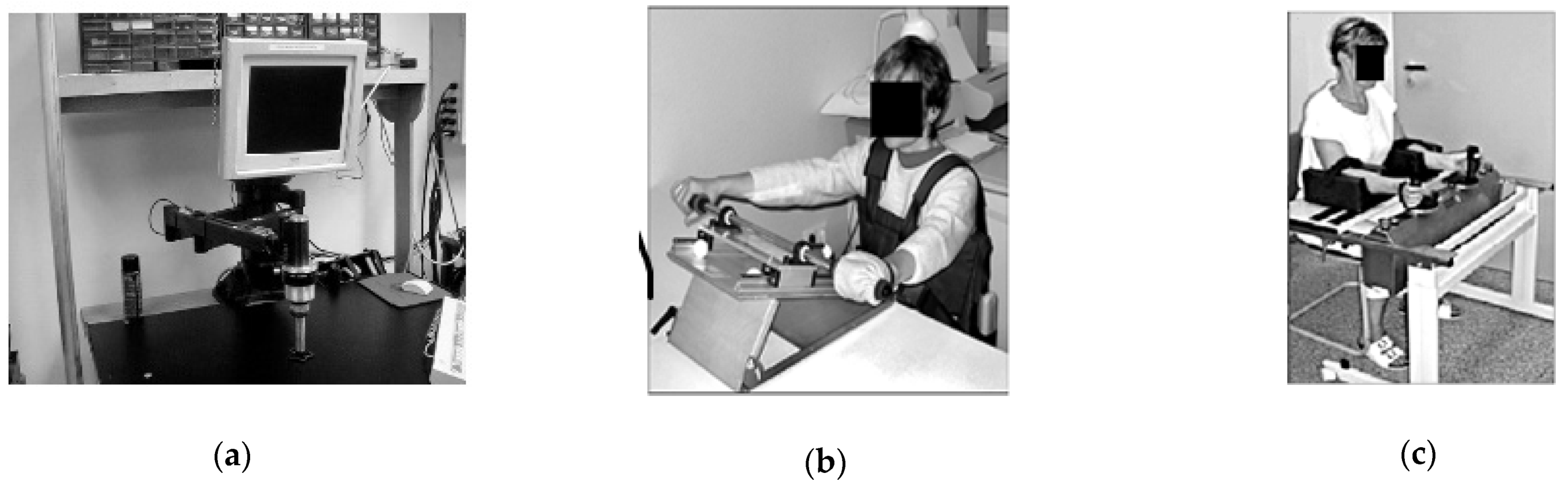
8]. Examples of these early mechatronic rehabilitation devices include the MIT-MANUS, Nudelholz, and Bi-Manu-Track systems (
Figure 1). These devices were designed with motion parameters explicitly chosen for each patient and could monitor rehabilitation progress. However, a significant limitation of these solutions was the inability to perform the full range of motion required for comprehensive rehabilitation.
To address this limitation, exoskeleton systems were developed. These systems feature rotation axes compatible with human anatomical axes, making them resemble human limbs. By attaching to the limb at multiple points, exoskeletons can support movements across different limb segments [
9,
10,
11,
12]. Reconfigurable systems offer an alternative approach, notable for their adaptable mobility, often called degrees of freedom (DoF) in kinematic chains. Even with reduced mobility (e.g., W = 3 DoF), these systems can facilitate critical wrist and forearm movements, including palmar and dorsal flexion, wrist adduction and abduction, and forearm pronation and supination [
13]. Additionally, systems for tracking and supporting hand movements have been extensively developed [
14,
15,
16].
The use of rehabilitation devices in therapy can potentially overcome certain limitations of manual therapy, such as inconsistent movement repetitions and difficulty in tracking progress. The rehabilitation process can be customized to meet individual needs by immersing the patient in a virtual environment. Numerous studies have validated the effectiveness of integrating virtual reality and psychological elements in rehabilitation devices [
1,
17].
However, rehabilitation remains a lengthy, complex, and costly process. It requires significant engagement and cooperation from both the patient and the physiotherapist and an individual approach adapted to each patient, complicating the automation of exercises. In systems of this type, the precise replication of motion is critically important. Predictive models are often used to achieve this precision [
18]. The issue of the influence of frictional forces and gravity is well known [
19] and has been extensively described in the context of surgical manipulators [
20,
21]. Despite these advances, significant improvements can be made by directly measuring the actual position of the device and the active torque during operation.
In response to these challenges, this study focuses on enhancing the movement quality by addressing the influences of friction forces and gravity. Research on a novel rehabilitation system, the Mechatronic Rehabilitation Device (MWR—named after first letters in polish: Mechanizm Wspomagania Rehabilitacji), began in 2014 at the Wroclaw University of Science and Technology [
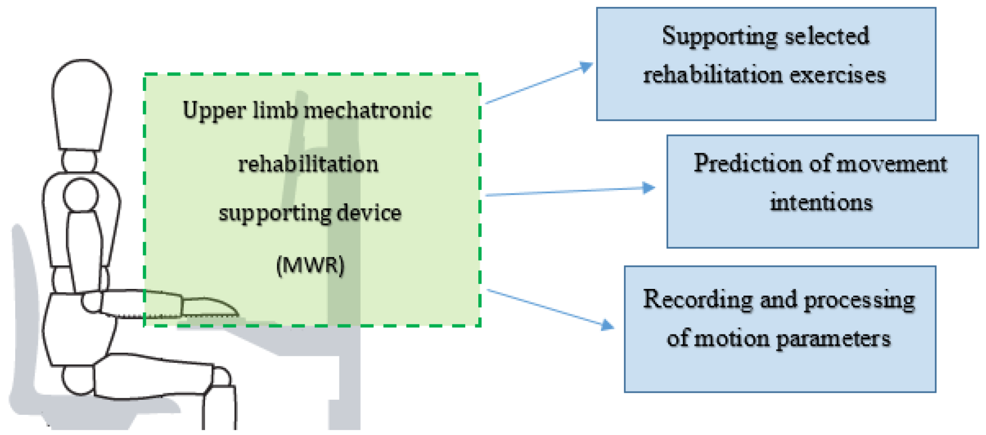
22]. The MWR system was developed with a modular structure, allowing it to function as two separate rehabilitation devices. Building upon the initial concept [
23], a new sensor system was added to measure the forces resulting from patient interaction. The MWR system supports both passive and active rehabilitation exercises and is capable of measuring, recording, and analyzing motion parameters and external loads during exercises (
Figure 2). This capability enables the device to adapt to the patient’s specific needs and provides detailed data for tracking rehabilitation progress.
2. Influence of External Factors and Gravity on the Movement of the MWR Mechanism
In order to enhance movement quality and address the influence of friction forces and gravity on the Mechatronic Rehabilitation Device (MWR), it was necessary to conduct detailed experimental studies. The study began by planning the experiment and investigating the mechanical parameters of the device.
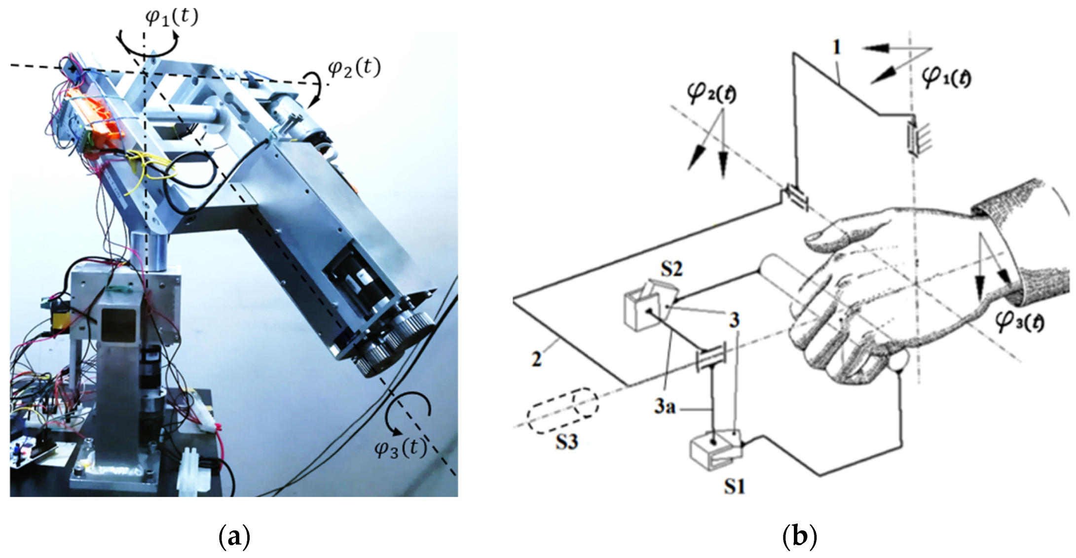
The measurement system of the MWR consists of incremental encoder sensors located on the axes of each supported movement: the pronation and supination
, palmar and dorsal flexion
, as well as adduction and abduction
of the hand (
Figure 3a). These encoders have a 12-bit resolution, which translates into 4096 impulses per rotation. This, in turn, translates into an accuracy of 0.088°. This is a sufficient number for this application.
In the MWR system, it was possible to measure the active torque in the drives for individual axes by using current sensors (ASC712, IDUINO, Riga, Latvia) and utilizing the characteristics of the motors. A significant advantage of the MWR was the ability to measure external loads thanks to the sensor grip (
Figure 3b). The grip had aluminum strain gauge beams S1 and S2 and a torque sensor S3 DFM22 Series (NCTE AG
®, Oberhaching, Germany). This enabled real-time control of the load with which the patient acted on the system.
Measurements from the sensors were transferred to a microcontroller, which was responsible for communication between the controlling computer (P.C.) and the sensory system. The measuring system consisted of a microcontroller from the NUCLEO family with an STMF303RE processor (STMicroelectronics, Geneva, Switzerland) operating at a frequency of 72 MHz.
The S3 torque sensor was directly connected to the microcontroller. In order to read the measurements from the strain gauge beams S1 and S2, it was necessary to use an operational amplifier. An industrial WTD-11-U amplifier (P.P.H. WObit E.K. Ober s.c., Pniewy, Poland) with a voltage output was used.
The research aimed to determine the actual parameters of the device, particularly the impact of the weight of individual components and friction between the moving elements.
In the studies, the object of control (regulation) was the angular position in the axes:
(t),
, and
. It related to assisted hand movements. Firstly, the characteristics of the device, without patient interference, using four set signals were examined, two of which consisted of achieving a given position (movement starting from the initial to a given position):
where
—linear function describing the end position in
i = 1, 2, 3 axes,
—sinusoidal function describing the end position in the
I axis,
—end position in the
I axis,
—initial position in the
I axis, and
—duty cycle.
The second variant consisted of one complete repetition. This meant achieving the specified angular position
from the initial position
in the movement
T1 time and then returning in
T2 time:
where
—linear function describing the end position and return in
i = 1, 2, 3 axes,
)—sinusoidal function describing the end position and return in the I axis,
—time to achieve end position, and
—time for a return to the initial position.
At the beginning of the research, the mechanism was set in the initial position
(
Figure 4a,c,e), considering the maximum safe ranges of motion for the given movement. They were, respectively, as follows:
,
,
.
Then, the end positions
were adopted (
Figure 4b,d,f). In this way, the range of movements in the experimental studies were determined:
,
,
.
Figure 4.
Range of motion for axis: initial positions (a,c,e) and end positions (b,d,f) for i = 1, 2, 3 for an anatomical range of motion, where the position of the hand is in the anatomical position of the body.
Figure 4.
Range of motion for axis: initial positions (a,c,e) and end positions (b,d,f) for i = 1, 2, 3 for an anatomical range of motion, where the position of the hand is in the anatomical position of the body.
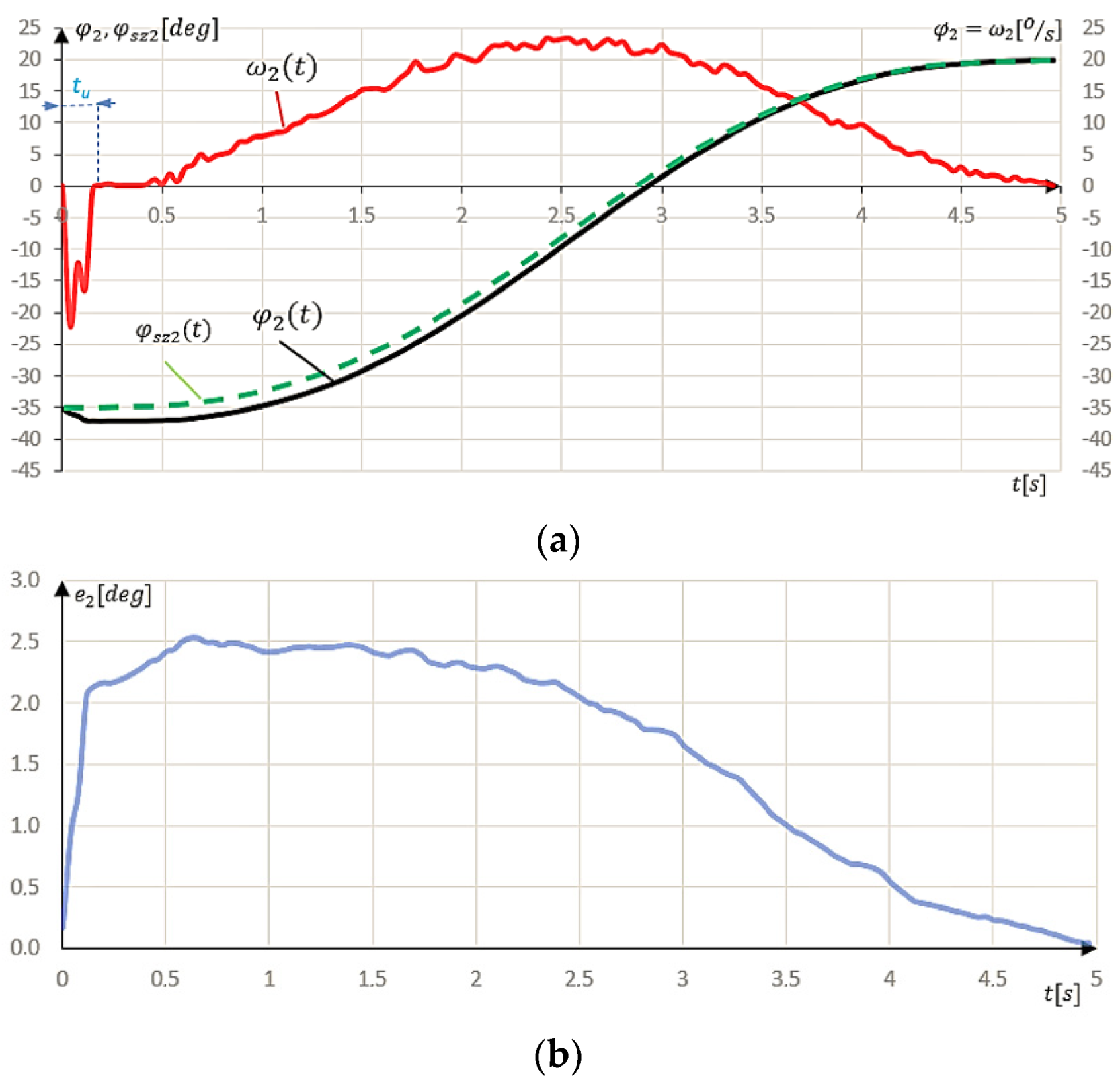
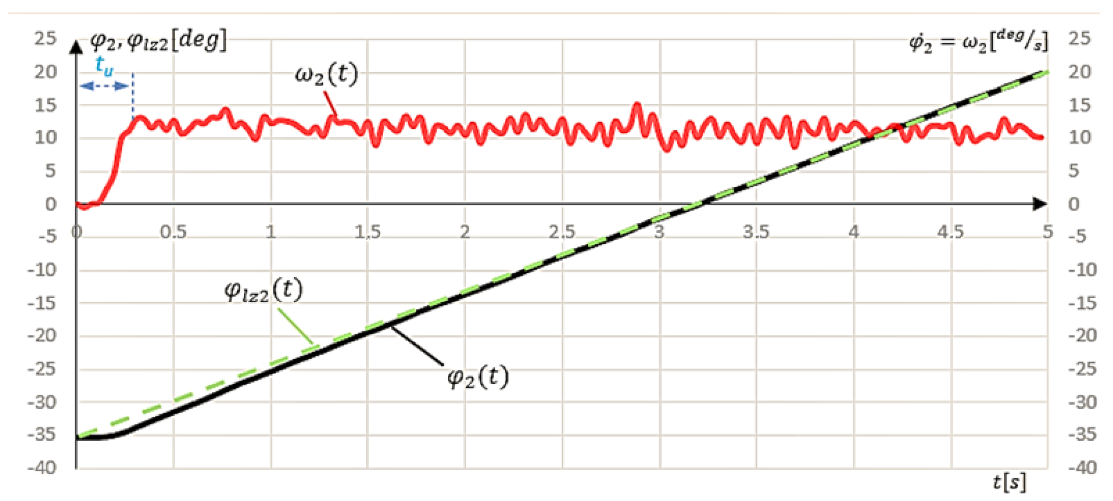
The research started with the linear input signal for all axes by the given assumptions. The experiment time was . The mechanism handle was not loaded during the tests. The research began with setting the initial position . Then, the system was stopped, the boundary and safety conditions were checked, and the set signal , the end position , and the controller settings were loaded. After checking the correctness of the above input data, the experiment was carried out, which consisted of exciting the movement by the input signal of .
Analyzing the characteristics of the individual axes of the mechanism (
Figure 5), it can be observed that only in the case of the
axis was there a sudden drop in angular velocity at the beginning of the movement (
Figure 5b). It reached the value of
= −13.15 deg/s for
t = 0.05 s. This was due to the mass of the elements, which the system must move at the start. The control system set the initial position
and then stopped the mechanism. Therefore, a precise active torque M
2 was required so that the mechanism started from this position. The angular velocity stabilized after
tu = 0.25 s. After reaching the set angular velocity value, the maximum difference between the actual value
and the calculated
was a maximum of 2.05°/s. The position error increased until the angular velocity stabilized, then decreased, reaching the set value
with each step.
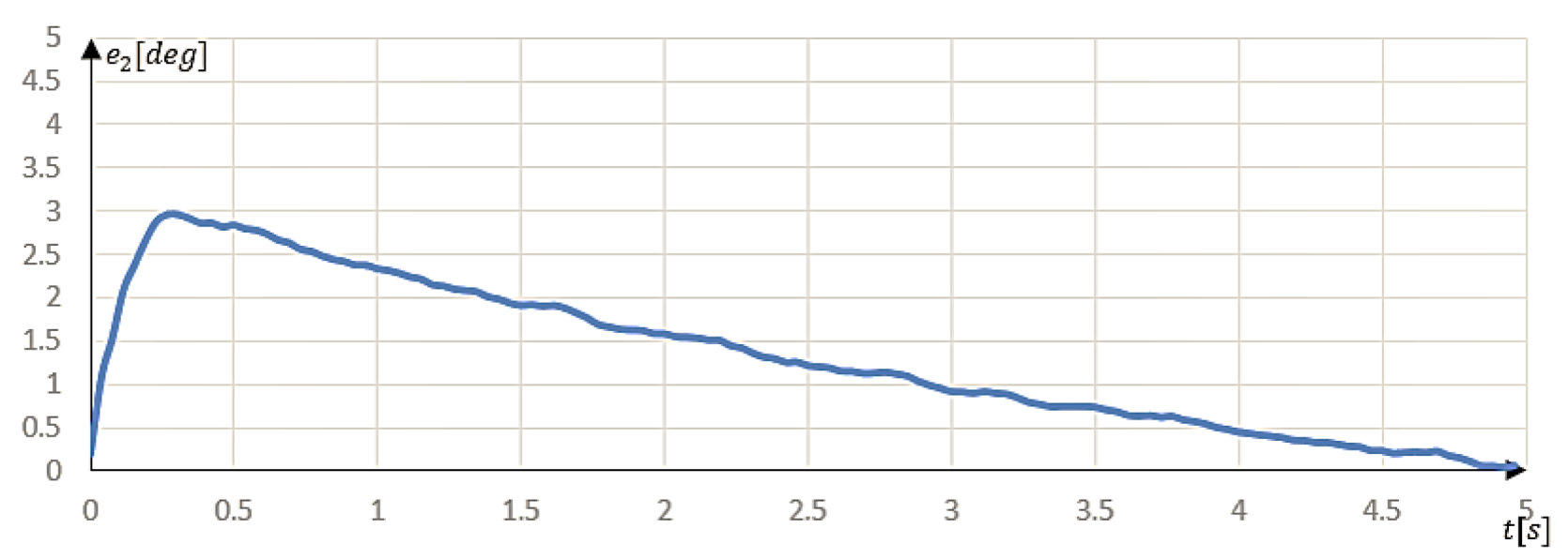
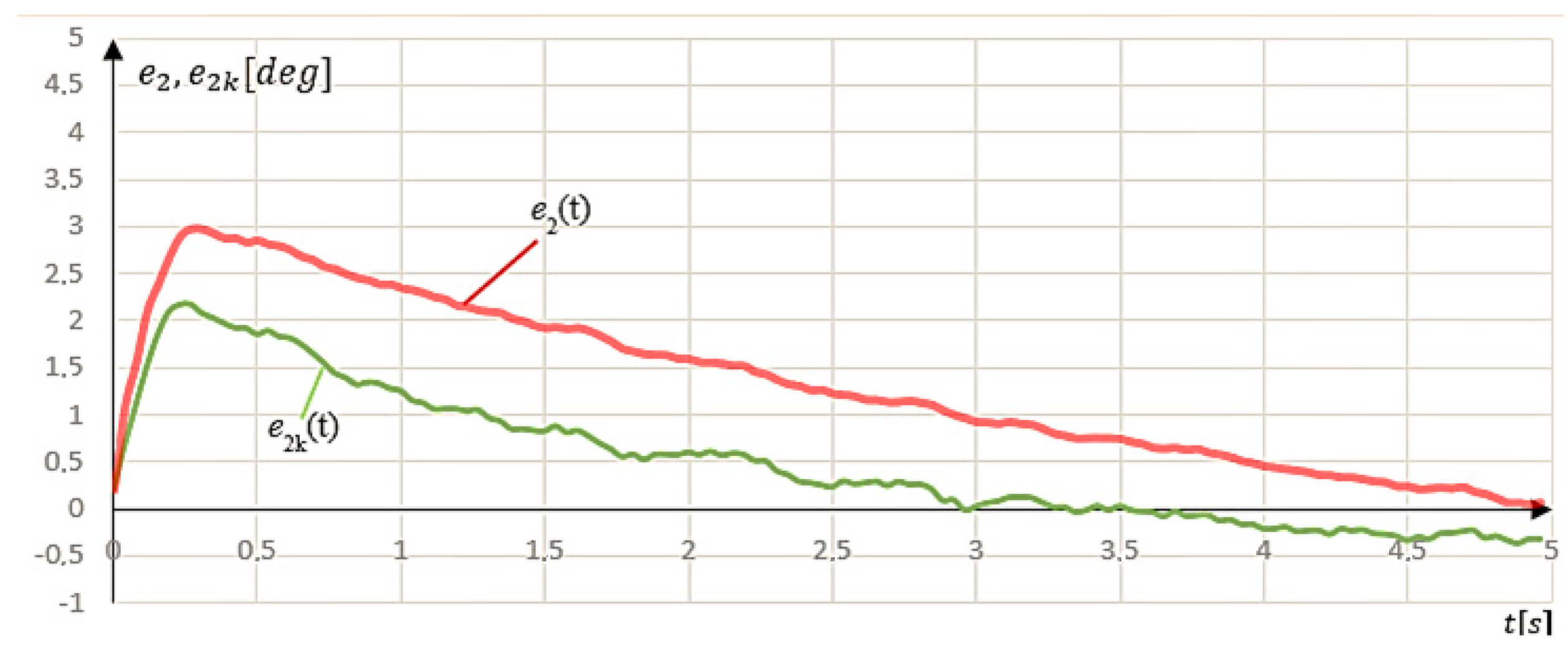
The maximum value of the position error
2.95° was for
t = 0.25 s, while the minimum value
0.05° occured for
t = 4.90 s (
Figure 6).
The following experiment consisted of reaching the given angular position and returning to the initial position defined by the function
. To examine the system’s response at higher angular velocities, the total motion duration was determined as
7 s. Consequently, it was required that the mechanism reach the predetermined position
3.5 s and then return to the original position
within
3.5 s. The experimental data of the
axis, under the application of linear actuation for the complete cycle of
, are shown in
Figure 7a.
Using a linear input signal, a sharp decrease in the angular velocity
right at the start of the test, dropping to −8.55° per second at 0.25 s, can be noticed. This caused a slight positioning error in the mechanism right after it started (−0.4°). Improvement can be seen when comparing this to the results from using the linear input signal
. However, angular velocity stabilized after 0.54 s, which was a disadvantage because a higher angular velocity was set in the experiment. After reaching the maximum position (
20°), a sudden change in the angular velocity
can be noticed. This also resulted in angular position oscillations, which decreased to t = 4.25 s (
to = 0.75 s). This was caused by the beginning of the second phase of the movement, in which there was a step change in the set speed
. The position error
increased until the angular velocity stabilized, then decreased until the system reached the highest position (
20°). The maximum value of the position error
was 2.55° for t = 3.65 s, while the minimum value was 0.56° for t = 3.50 s (
Figure 7b).
The next stage consisted of enforcing the sinusoidal input signal for the (t) axis. Such an input reflects the real motion much better because it can distinguish between two phases of motion (acceleration and deceleration). The tests were conducted for the same parameters as the linear reference inputs. The results are shown below.
For the sinusoidal input signal, one can observe a decrease in the angular velocity
at the beginning of the movement. It is similar to the linear input. Time
is also almost identical to a linear signal and is
= 0.25 s (
Figure 8a). The position error
increases significantly at the beginning of the movement until t = 0.65 s, where the regulation system gradually compensates. For the first half of the movement, it remains at about 2° and then decreases (
Figure 8b).
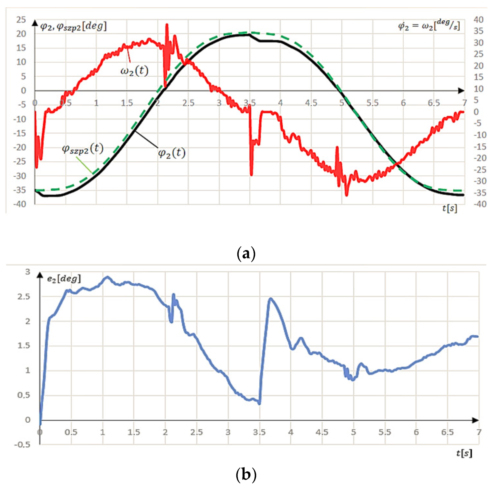
The subsequent tests were performed for one complete cycle, according to the
function. The range of motion
and its parameters
3.5 s were the same as for the case of the linear input signal (
Figure 9).
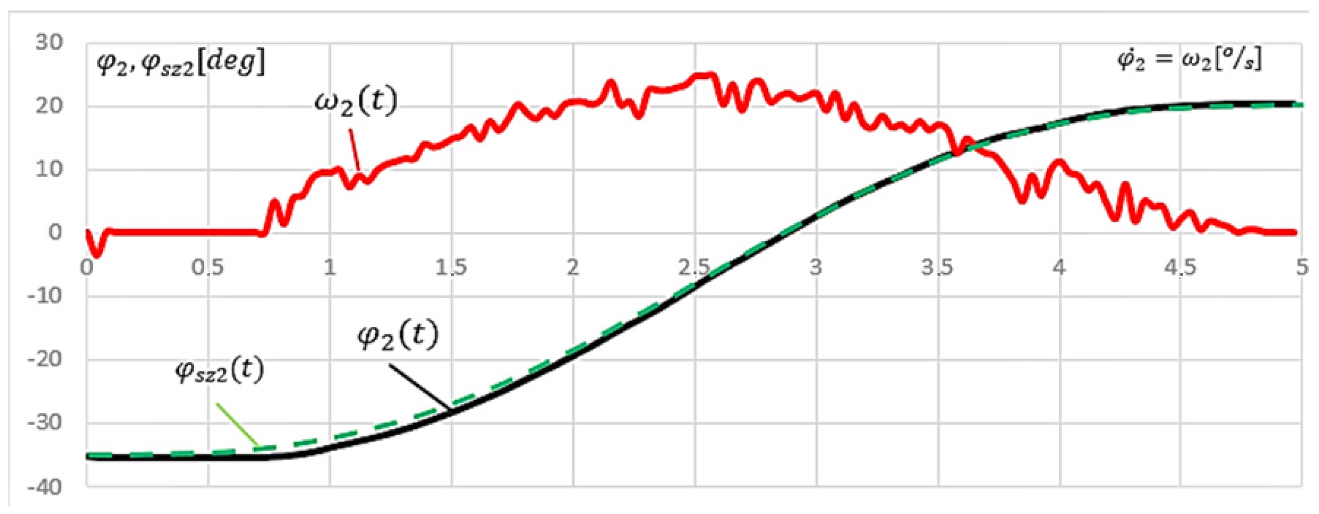
With a sinusoidal input signal
, the angular velocity
decrease can be observed at the beginning of the movement. It reached the value of −23.85 °/s for t = 0.025 s and was much larger than in the case of the previous study. This resulted in an error in the angular position
of the mechanism immediately after the start (−2.02°). The reason for this was the higher input value of the angular velocity (
Figure 9a). The system had a problem with maintaining the angular velocity at the beginning of the movement (t = 0), which was related to the mass of the mechanism. For t = 2.10 s and t = 4.95 s there were slight speed oscillations caused by the need to reduce the angular velocity
(stabilizes after 0.15 s). The moment when the final position
was reached (t = 3.5 s) deserves special attention. At this point, the system needed to change its direction of motion. The error associated with this task resulted from changing the direction of motion and overcoming friction forces. The consequence was the disruption of the angular velocity
, which stabilized after 0.6 s. The characteristics of the position error for a sinusoidal and linear input signal when performing one complete repetition (
Figure 7b and
Figure 9b) were similar. The position error
(t) did not exceed 3°, increased at the beginning of the first and second phases, and decreased at the ends of these movement phases.
3. Enhancing Movement Quality by Implementing a Compensation Function
The experimental studies have shown the significant impact of the mass of the components in the axis on the quality of movement. In order to improve the operation of the system, this impact had to be compensated for. For this reason, special procedures were developed: analytical and experimental.
Firstly, an analytical method was used to determine the torque acting on the
axis. At that time, friction forces between the elements were omitted, and the method served as a verification for the experimental method. The masses and centers of masses of the individual elements were determined, and then their lever arms were calculated (
Figure 10,
Table 1).
The maximum analytically calculated axis load related to the gravity and mass of the elements was 14.04 Nm. This was calculated for the angular position .
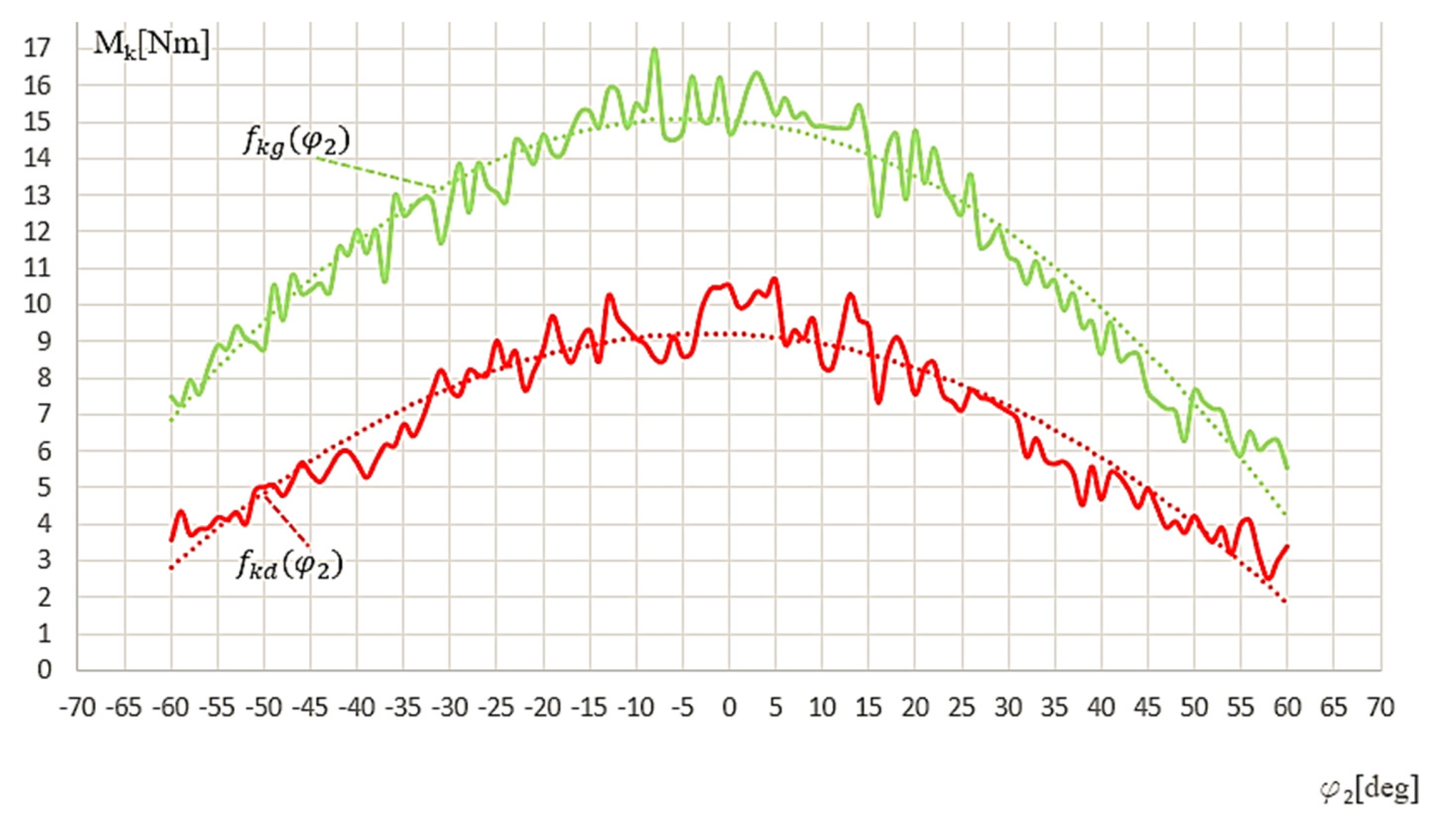
The second experiment consisted of determining axis load experimentally by using the drives’ characteristics (characteristics of the generated torque depending on the current consumption) and measuring the current via the current sensor. The experiment began with setting the range of motion. For the research, the angular range for the axis was set to , where is the examined angular position of the mechanism.
The procedure’s main goal was to determine the active torque () needed to keep the mechanism in a given angular position in the axis. The torque was determined based on the measurement of the current consumed by the drive and its characteristics. The mechanism position changed by one degree at a time. The measurement was carried out in two opposite directions of movement for the axis, i.e., it was the torque needed to move the mechanism upwards and downwards from the stopped angular position. The difference between these two quantities defined the area where the mechanism remained motionless. The size of this area was related to the forces of static friction, motion resistance (mainly of the gear), and the mass of the mechanism’s components.
The correct definition of this area is a critical element of the system’s operation. It is possible to read the external force vector acting on the device during movement. This vector determines the direction and value of the force with which the patient acts on the handle. Therefore, it can be set for the appropriate compensation. The results of determining the compensating functions are presented in
Figure 11.
By approximating the obtained characteristics with a quadratic function, a compensating function was obtained for the upward movement of
and downward movement of
:
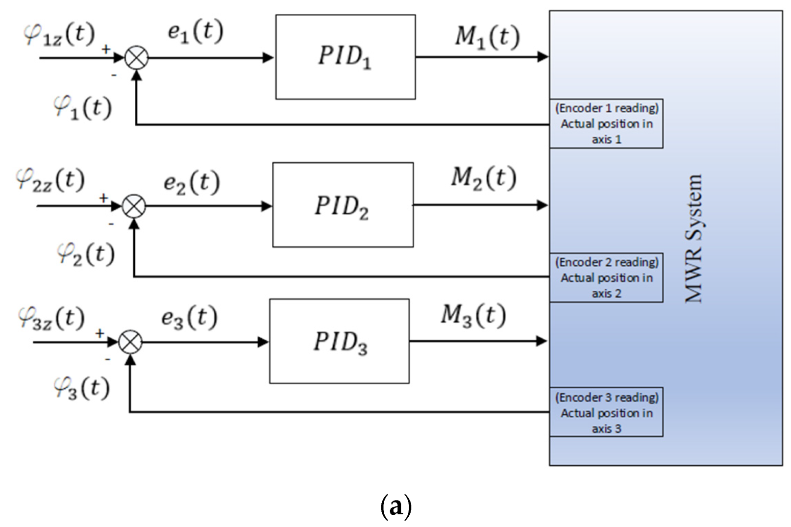
After the experiments, a modification was introduced to the
axis control system (
Figure 12). In the control system, a compensating function
was added to the control torque
, obtaining the control torque
.
In order to examine the improvement of the mode performance, the experiment was performed again for the linear input signals
and
. The linear input tests were performed for the same adopted parameters
and
and the movement time
, as well as for the movement without compensation (
Figure 13).
Analyzing the linear input signal, a significant improvement can be observed at the beginning of the movement. The position error at the beginning of the movement for t = 0.4 s was . However, the angular velocity stabilization time did not improve and was s. The integral criterion of the absolute value of the error signal was used to assess the improvement of the system’s performance.
For a linear set signal, it was
. At the same time, after adding the compensating function, it decreased by nearly 53% to
(
Figure 14). For a linear set signal, the introduction of a compensation function resulted in a significant improvement in the motion quality.
However, the velocity error was investigated by
. This time, adding the compensating function resulted in an increase to
(
Figure 15). However, when investigating
and
, one can notice an improvement in the operation. Adding the compensation function resulted in stronger oscillations over the given velocity signal, and therefore, the quality factors lowered; however, what was the most visible was how it reduced the maximal error at the beginning of the movement.
In the next step, an experiment with the sinusoidal input
was performed for the same adopted parameters as for the test without the compensating function (
Figure 16).
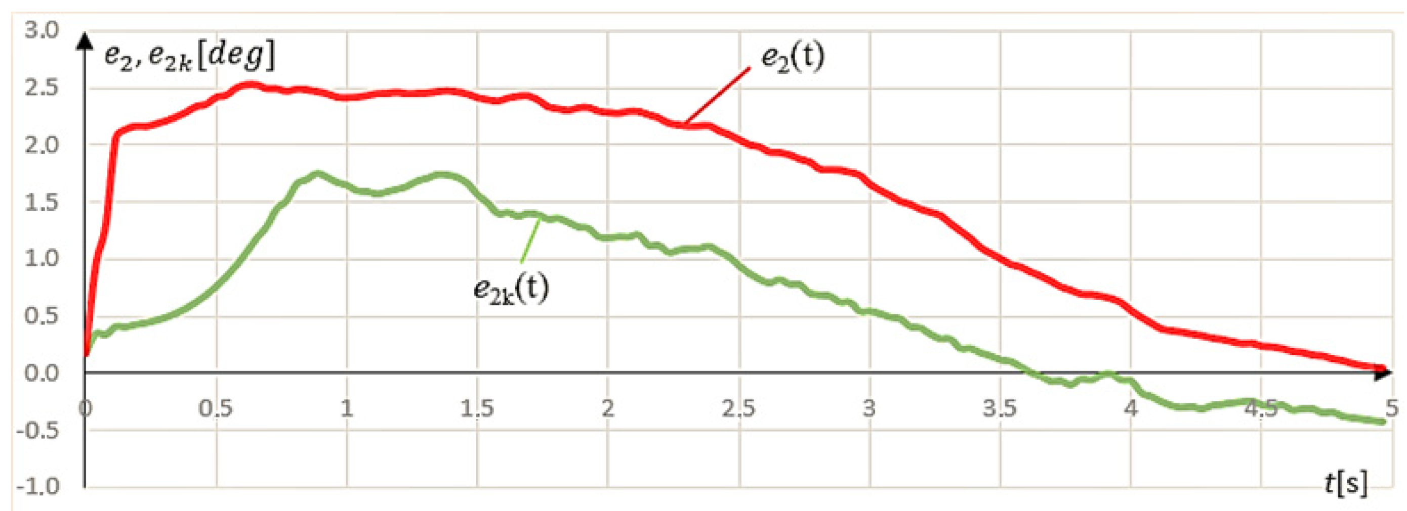
In this case, it was also impossible to eliminate the occurrence of position errors at the start of the movement. The value of the error
, for
t = 0.05 s, was equal to
. The integral criterion of the absolute value of the error signal was also used to assess the improvement of the system’s operation. For a sinusoidal set signal, it was
, while after adding the compensating function, it decreased by nearly 52% to
(
Figure 17).
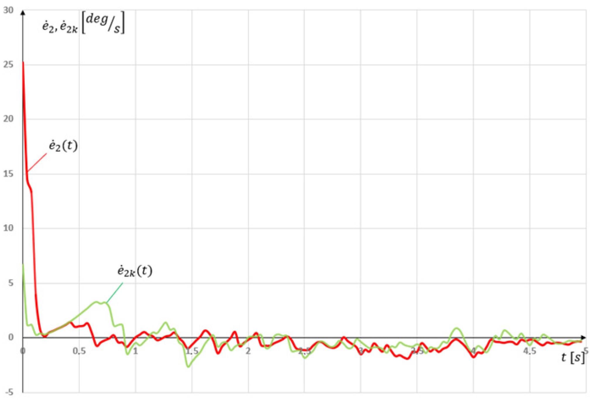
In this case, the angular velocity error was represented by
. This time, adding the compensating function resulted in a decrease to
(
Figure 18). However, when investigating
and
, one can notice different situations than in the linear input; however, these values were low and indicated oscillations among the given angular velocities. Adding the compensation function resulted again in a reduced maximal angular velocity error at the beginning of the movement.
The evaluation of the control quality in the case of the MWR device was complex. The integral criterion of the absolute value of the error signal showed a significant improvement in angular position. However, when investigating the angular velocity error in the case of the linear input, the integral was raised. This resulted in strong oscillations among given angular velocity signals and did not affect the overall quality of the movement improvement shown in the integral position error.
4. Discussion
This study aimed to enhance the movement quality of the Mechatronic Rehabilitation Device (MWR) by addressing the influences of friction forces and gravity, particularly on the φ2 axis responsible for palmar and dorsal flexion of the hand. The experimental results revealed that the mass of the mechanism’s components, and external factors, such as gravity, significantly affected the control system’s ability to maintain the desired angular position and velocity in the φ2 axis.
Initially, the control system exhibited challenges in achieving smooth motion, with noticeable position errors and oscillations during both linear and sinusoidal input signals. The angular velocity ω2 showed sudden drops at the start of movements, indicating the system’s struggle to overcome inertia and friction without compensation.
By implementing compensation functions and , derived from the experimentally determined drive torques needed to maintain specific angular positions, the control system was modified, taking into account the gravitational and frictional influences on the φ2 axis. Introducing these compensation functions led to a significant improvement in movement quality. Specifically, the integral of the absolute value of the position error decreased by more than half for both linear and sinusoidal inputs after compensation, indicating enhanced accuracy and smoother motion.
The improved performance underscores the importance of addressing mechanical factors in the design and control of rehabilitation devices. By compensating for the weight of the mechanism and frictional forces, the MWR device achieves more precise movements, which are critical for effective rehabilitation therapy. This enhancement improves patient safety and comfort and allows for the more accurate tracking of rehabilitation progress, potentially leading to better therapeutic outcomes.
However, the study has limitations that warrant further investigation. The compensation functions were developed based on experiments conducted without patient interaction. Future studies should involve clinical trials with patients to evaluate the effectiveness of the compensation strategy in real-world rehabilitation scenarios. Additionally, while the φ2 axis was the focus due to its significant impact, exploring compensation strategies for the other axes (φ1 and φ3) could provide a more comprehensive improvement in the device’s overall performance.


