UaVirBASE: A Public-Access Unmanned Aerial Vehicle Sound Source Localization Dataset

Abstract

This article presents UaVirBASE, a publicly available dataset for the sound source localization (SSL) of unmanned aerial vehicles (UAVs). The dataset contains synchronized multi-microphone recordings captured under controlled conditions, featuring variations in UAV distances, altitudes, azimuths, and orientations relative to a fixed microphone array. UAV orientations include front, back, left, and right-facing configurations. UaVirBASE addresses the growing need for standardized SSL datasets tailored for UAV applications, filling a gap left behind by existing databases that often lack such specific variations. Additionally, we describe the software and hardware employed for data acquisition and annotation alongside an analysis of the dataset’s structure. With its well-annotated and diverse data, UaVirBASE is ideally suited for applications in artificial intelligence, particularly in developing and benchmarking machine learning and deep learning models for SSL. Controlling the dataset’s variations enables the training of AI systems capable of adapting to complex UAV-based scenarios. We also demonstrate the architecture and results of the deep neural network (DNN) trained on this dataset, evaluating model performance across different features. Our results show an average Mean Absolute Error (MAE) of 0.5 m for distance and height, an average azimuth error of around 1 degree, and side errors under 10 degrees. UaVirBASE serves as a valuable resource to support reproducible research and foster innovation in UAV-based acoustic signal processing by addressing the need for a standardized and versatile UAV SSL dataset.

1. Introduction

Humans possess an innate ability to localize sounds in their environment, seamlessly determining the direction and distance of a sound source. This ability is crucial for interpreting and responding to dynamic scenes, as it allows for the integration of auditory and visual information. Inspired by this human capability, sound source localization (SSL) has emerged as a fundamental area of research in acoustic signal processing [1]. It has a broad range of applications, from robotics [2], urban noise monitoring [3], and visual scene analysis [4] to wildlife monitoring [5] and IoT systems [6].

In recent years, the growing prevalence of unmanned aerial vehicles has further amplified interest in SSL, particularly for detecting and localizing umanned aerial vehicles (UAVs) in scenarios such as security operations, surveillance, airspace monitoring, and even military applications [7]. However, UAV localization introduces unique challenges, including the blending of rotor noise with environmental sounds, varying flight altitudes, rapid and dynamic movements, and strong ego-noise from motors and propellers, which result in low signal-to-noise ratios (SNRs) and dynamic acoustic transmission paths [8]. To address these complexities, UAV localization systems often rely on various technologies, including RF radio, radar, acoustic, vision-based methods, or fusion sensors [9]. Each of these approaches has unique advantages and limitations [10].

RF radio methods are widely used due to their cost-effectiveness and suitability for long-range detection, but they can be affected by signal interference or deliberate suppression by UAVs [11]. Radar systems, on the other hand, are robust and provide wide spatial coverage and high angular resolution [12]. Yet, they face challenges distinguishing UAVs from other low-altitude, slow-moving objects such as birds. Vision-based methods provide high precision and excellent tracking capabilities; however, they struggle in conditions of low visibility or environments with visual obstructions [13]. Acoustic localization using microphone arrays complements these technologies by leveraging the unique rotor noise generated by UAVs, which is difficult to conceal and remaining unaffected by low visibility or radio interference. However, acoustic methods face challenges in environments with high background noise levels, where distinguishing UAV sounds from other ambient sounds can be difficult. Additionally, the range of acoustic detection is typically shorter compared to RF or radar-based systems, limiting its application in large-scale monitoring scenarios [14].

Fusion sensor systems, which integrate data from multiple modalities, such as combining two [15,16,17] or three sources [18], have demonstrated their effectiveness in overcoming the limitations of individual methods. By leveraging the complementary strengths of RF, radar, vision-based, and acoustic techniques, these systems significantly enhance the reliability and accuracy of UAV detection and localization, especially in complex and dynamic environments [9].

However, despite their effectiveness, fusion systems can be resource-intensive, requiring substantial hardware, integration, and computational infrastructure investment. This makes them less feasible for cost-sensitive applications. In contrast, acoustic localization stands out as a more cost-effective alternative. With relatively inexpensive hardware, such as microphone arrays, and the ability to utilize computationally efficient classical algorithms, acoustic systems provide a practical solution for budget-conscious UAV monitoring scenarios. Despite their limited detection range and susceptibility to noise compared to RF or radar-based methods, their affordability and simplicity make acoustic localization an appealing choice for applications with constrained budgets.

To address the challenges of sound source localization, numerous methods have been developed, broadly categorized into classical approaches and artificial intelligence (AI)-based methods [19]. Classical techniques, such as Time Difference of Arrival (TDoA), Direction of Arrival (DoA), and beamforming, rely on well-established signal processing frameworks [20]. These methods are computationally efficient and perform well in controlled conditions but often face limitations in dynamic, noisy, or complex environments.

On the other hand, AI finds applications in many fields, ranging from digital watermarking [21], 3D printing material optimization [22], and process planning [23] to deepfake generation [24] or victim verification [25], showcasing its versatility across diverse domains. In acoustics, AI-based methods leverage the power of machine learning and deep learning models to capture intricate spatial and acoustic relationships. These approaches offer enhanced robustness and adaptability, particularly in environments with significant background noise or non-stationary sound sources. By learning directly from the data, AI-driven methods address many of the challenges associated with classical approaches, although this is at the cost of requiring large, high-quality datasets [26] and considerable computational resources.

Recognizing the growing prominence of artificial intelligence and its potential to transform acoustic localization, we undertook a significant initiative: creating a dedicated sound dataset for UAV localization. This dataset was meticulously designed to address the multifaceted challenges of UAV SSL. It includes UAV rotor noise recorded at varying altitudes, distances, and angles relative to the microphone array—front, back, right, and left of the drone—and background noise from the urban environment. The primary goal of this work was to develop a structured, extensible, and fully replicable experimental setup for UAV localization—including the dataset, hardware configuration, and training process—that reflects the complexities of real-world spatial audio recording. While this first version includes a single UAV, it establishes a replicable framework and serves as a foundation for broader multi-UAV datasets. In doing so, it enables the training and evaluation of AI algorithms designed for UAV localization, fostering the development of more robust and adaptive systems. The dataset also enables the classification of the UAV’s orientation relative to the microphone array, determining whether the drone is positioned at the front, back, right, or left. These detailed positional data allow for the more precise determination of UAV locations, supporting advancements in localization techniques.

Although several UAV acoustic datasets have been published [27,28,29,30,31,32,33,34,35,36,37,38], they primarily focus on detection or classification tasks and often lack spatial detail or comprehensive labeling. Many of these datasets contain mono or stereo recordings with limited metadata and are not designed for full sound source localization. In contrast, UaVirBASE offers high-resolution 8-channel audio captured at 96 kHz and a 32-bit depth, with detailed annotations covering azimuth, distance, height, and the drone’s relative side. This enables spatial reasoning and directional modeling far beyond the capabilities of existing datasets. Our initiative bridges a critical gap in available resources for the research community, emphasizing the importance of high-quality data in driving innovation and addressing the challenges of modern UAV monitoring requirements.

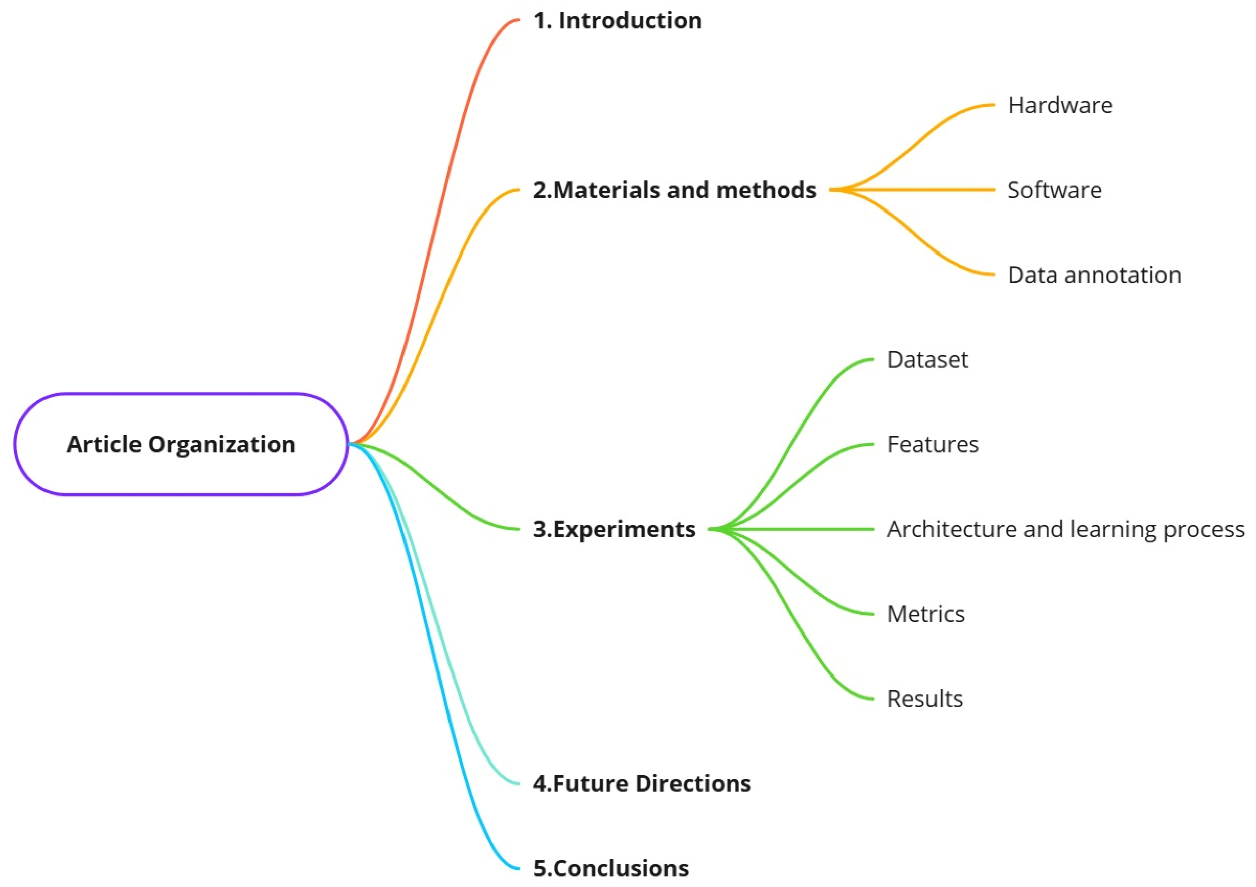
As shown in Figure 1, the structure of this article includes the following sections: Section 1 is the Introduction. Section 2, titled Materials and Methods, presents the hardware and software components used for data collection, along with the data annotation process. Section 3 details the experimental setup, including the structure of the UaVirBASE dataset, the selected audio features, the architecture and training process of the deep neural network model, the evaluation metrics used, and the results obtained. Section 4 discusses future directions, and Section 5 concludes the study.

2. Materials and Methods

To meet the specific requirements of high-resolution acoustic data collection for UAV localization, we developed a custom recording system tailored to this task. Existing commercial solutions lacked the necessary flexibility in terms of modularity, portability, and compatibility with various configurations and sensor types. Therefore, the system was built using a combination of commercially available components (e.g., microphones, audio interfaces, and cables) and custom-designed structural elements fabricated using Fused Deposition Modeling (FDM), which is a layer-by-layer 3D printing process [39].

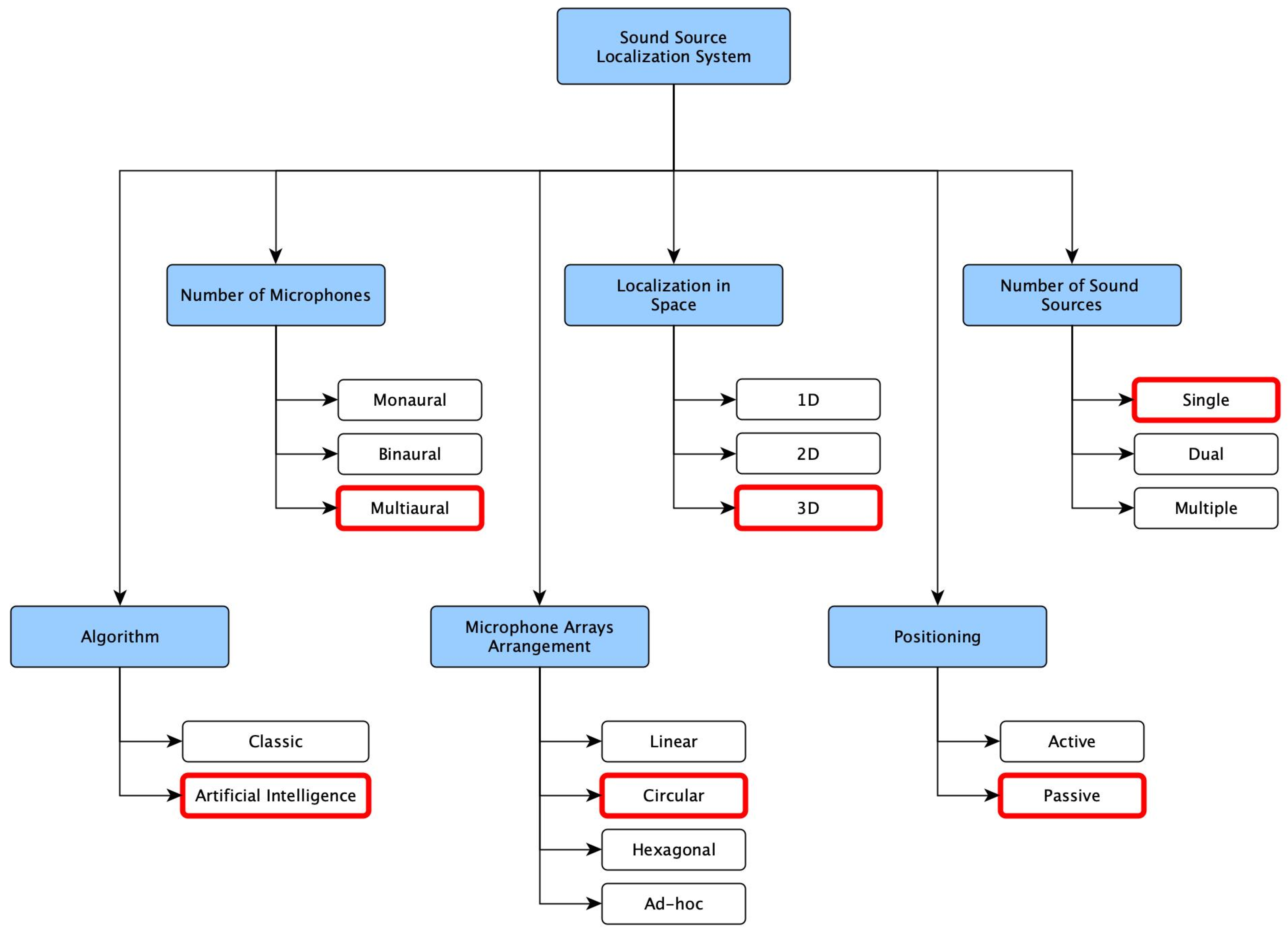
As with designing any system, we initially had to determine the essential parameters and establish a framework. By adopting the already proposed system of the classification of SSL systems [19] with minor modifications, we could streamline the process and guarantee that all necessary parameters were adequately captured. The selected algorithm could be omitted to create the dataset, as the dataset itself does not mandate its usage for either the classic or AI approach. However, there is an example in the later chapter of this article demonstrating the basic usage of the dataset in a neural network. Therefore, we have decided to mark it in the system summary in Figure 2.

Before deciding on the number of microphones, there is a change in the proposed categorization. While monaural and binaural designations were left unchanged, we bunched the number of microphones above that into one multiaural group. We decided to use a circular arrangement of eight microphones on two levels (four each). Another change in the graph regarding localization is the space category. There were now three groups with a defined number of dimensions. We decided to capture as much data as possible to categorize this system as 3D.

Finally, since the system relied solely on microphones and did not incorporate speakers or other sound-emitting devices for echolocation, it was classified as passive.

With this information, we proceeded with the specific hardware and configuration used. The selection of microphones influences further design decisions, including mounting methods and their localization, as well as the connections and hardware utilized for signal collection.

2.1. Hardware

For this study, we used a single UAV model—the DJI Mavic 3 Cine—which was sufficient to demonstrate and validate the recording system’s functionality. This drone was selected due to its commercial availability, stable flight behavior, and representative acoustic characteristics. The inclusion of additional UAV models is a concept planned for future work and can be integrated into the current system without major changes.

We opted to utilize microphones with a supercardioid pattern, as they offer superior noise rejection compared to omnidirectional microphones. While this choice may restrict the application of certain methods, such as TDoA, as the object’s sound may be more challenging to isolate when the microphone is facing away from it, it does provide additional information regarding direction. The microphone directed at the sound source will capture it more precisely. Given these considerations, we selected the Røde NTG2 shotgun microphone [40]. This microphone has a relatively high dynamic range of 113 dB and a frequency range of 20 Hz to 20 kHz. Although it does not encompass infrasound or ultrasound, it should be adequate to capture the diverse range of noises generated by the rotors of the UAV.

The next crucial component is the audio interface. It should be user-friendly and have sufficient connectivity to accommodate eight microphones. Additionally, it should have a high sampling rate and bit resolution. We chose to use the Behringer UMC1820 [41]. This interface surpasses the selected microphones for the available audio frequency band. Furthermore, it offers a 96 kHz sampling rate, which should provide sufficient audio quality for our purposes.

For static localization, we opted to refrain from utilizing Global Positioning System (GPS) technology. However, further research is underway to develop dynamic localization capabilities with UAVs in motion, utilizing high-resolution GPS data. Instead, we chose to employ conventional methods of distance measurement. For this purpose, we utilized a measuring wheel and verified the results using a laser rangefinder. This enabled us to determine the horizontal distance while the remaining components of the position were measured using sensors onboard the UAV.

Due to the multifaceted nature of sound wave propagation, influenced by factors such as temperature, humidity, and atmospheric pressure, we incorporated data from a local weather station. The strategic placement of the station at the recording location provided access to weather data and enabled the collection of wind conditions, including direction and speed. This additional information significantly enhanced our dataset and potentially facilitated the more effective de-noising of the recordings. However, we chose not to perform de-noising ourselves but instead provided the recordings in their raw, unaltered form. To facilitate the aforementioned data streaming for app development, we selected the SenseCap S212 8-in-1 Weather Sensor [42], which boasts a compact design while offering a comprehensive suite of sensors, easy mounting, and before-mentioned remote data streaming capabilities.

For data recording, we also decided to record the whole recording session “from the side”. We used Zoom h4essential [43] with two connected Behringer B-1 [44] microphones.

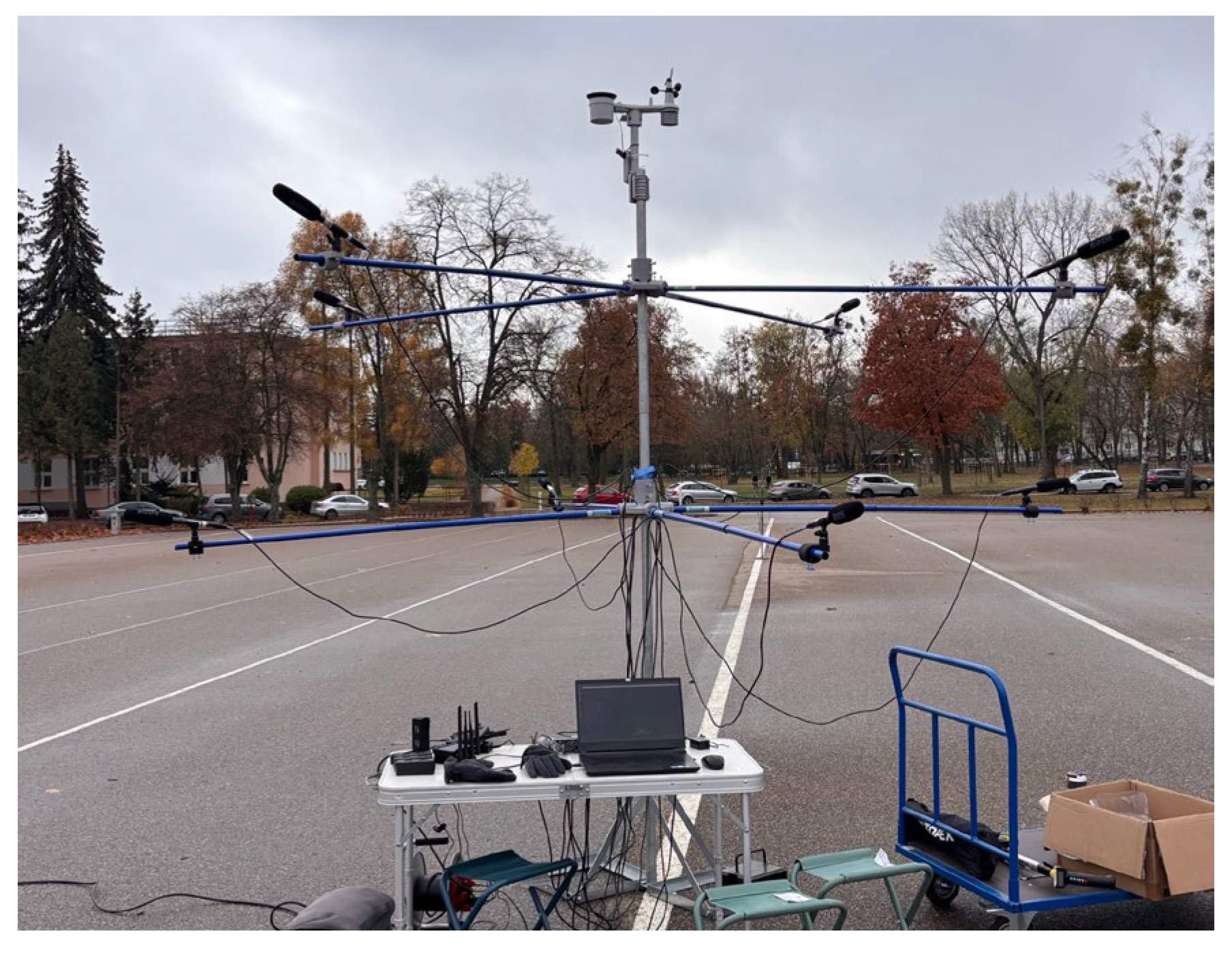
These are the primary “off-the-shelf” hardware components utilized in constructing a database. Now, let us proceed with describing how they were assembled for recording. We designated our recording rig as “Acoustic Head”; henceforth, we will refer to the constructed device by this name. In this setup, we recorded the DJI Mavic 3 Cine UAV (Figure 3).

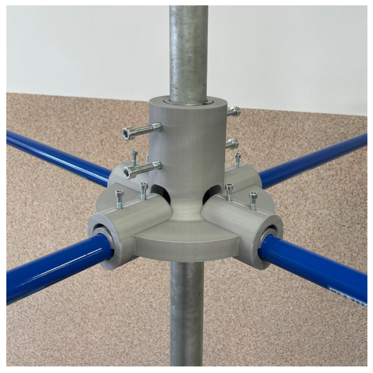
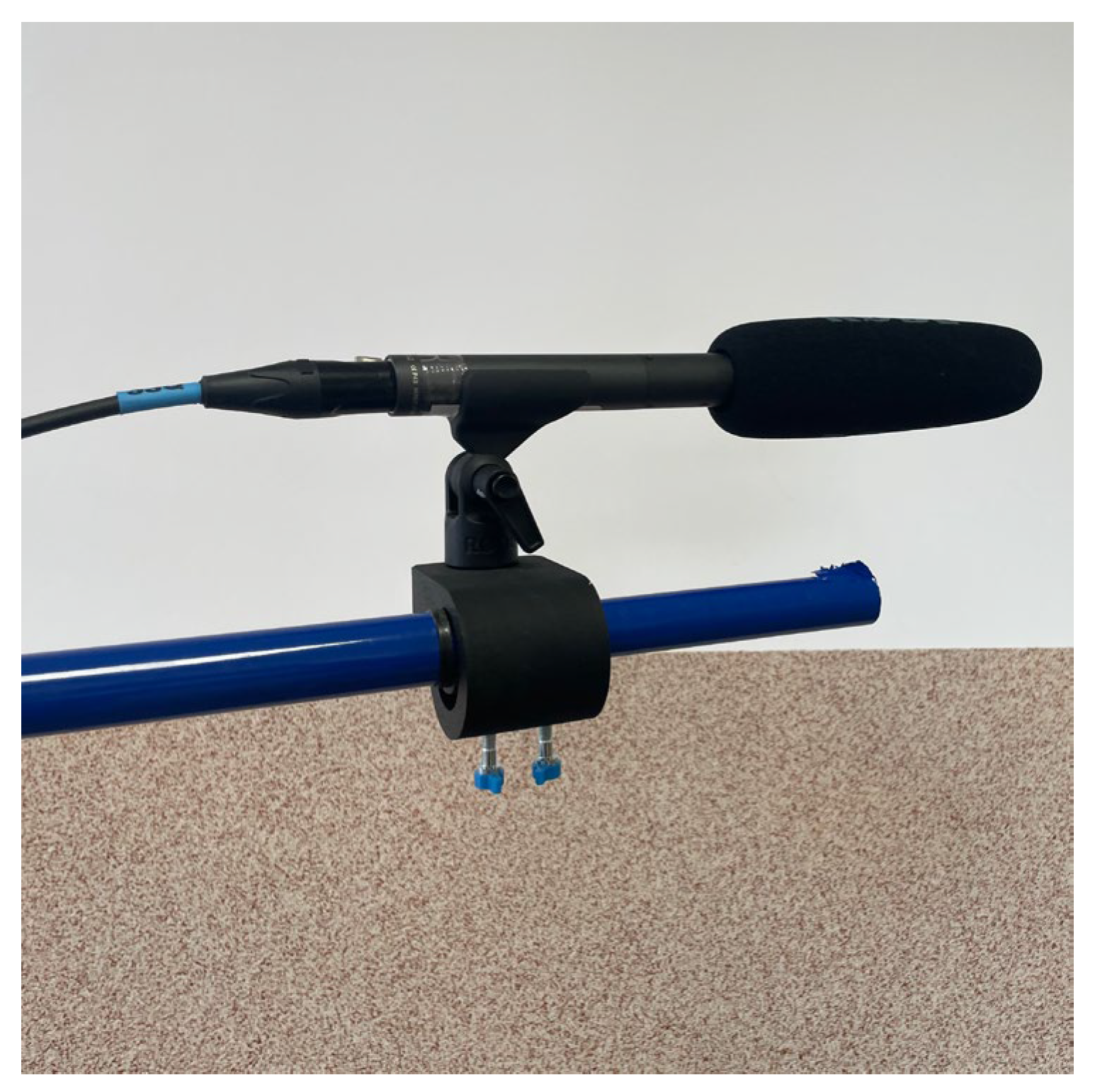
As previously mentioned, we utilized eight microphones divided into two levels (four microphones per level). Each level comprised four arms, with a microphone mounted on each arm (Figure 4).

These levels are independent, and the distance between them can be adjusted as per the requirement (Figure 5). Furthermore, each microphone can have its distance from the center changed independently of other microphones (Figure 6). Additionally, each microphone’s angle can also be selected.

Such a setup allows for easy configuration, switching microphone angles, and changing the distance from the center and the distance between levels.

A summary of the hardware components used in this study is provided in

Table 1. Hardware components summary.

Component	Model/Description	Key Specifications/Features	Purpose
UAV	DJI Mavic 3 Cine (DJI, Shenzhen, China)	Quadrocopter	Acoustic sound source
Microphones	Røde NTG2 (RØDE Microphones, Sydney, Australia)	Supercardioid, 20 Hz–20 kHz, 113 dB dynamic range	Directional sound capture
Microphone Mount	Custom dual-level frame (self-made)	Two levels (4 mics each), adjustable distance and angle	Spatial audio array configuration
Audio Interface	Behringer UMC1820 (Behringer, Zhongshan, China)	8 XLR inputs, 32-bit, supports 96 kHz sampling rate	Multi-channel audio signal acquisition
Secondary Recorder	Zoom H4essential (Zoom Corporation, Dongguan, China)	2-channel, 96 kHz/32-bit float	Whole session recorder
Weather Station	SenseCAP S2120 (Seed Studio, Shenzhen, China)	Temp, wind speed, humidity, barometric pressure, direction	Environmental metadata capture
Distance Measurement	Bosch GLM 150 C Laser (Bosch, Penang, Malaysia)	±1.5 mm accuracy, up to 150 m range	Drone distance positioning
Mounting Hardware	FDM 3D-printed components (self-made)	Custom brackets, arms, mounts	Microphone positioning and adjustment

.

2.2. Software

The creation of the UaVirBASE Recorder software (version 1.0) was motivated by a clear need to overcome the limitations of existing audio recording tools for scientific research. While widely used platforms like Audacity [45] provide basic recording functionalities, they lack the advanced features, flexibility, and precision required for complex experimental setups, such as sound source localization using microphone arrays. Our goal was to design a system that not only meets the technical demands of such experiments but also facilitates efficient data collection and ensures the integrity of the resulting datasets.

One of the primary challenges we faced was the inflexibility of commercial or open-source recording tools. Most existing solutions do not allow researchers to dynamically modify recording parameters such as the sampling rate, bit depth, or microphone configurations during an experiment. This lack of adaptability can hinder experimental workflows and limit the ability to capture data under varying conditions. Furthermore, many of these tools are tailored for general-purpose audio recording rather than the high-performance requirements of scientific studies.

Another critical limitation was the lack of automated data labeling in existing software. Labeling experimental data manually is time-consuming and prone to human error, especially when dealing with large datasets. For our research, which involves the creation of a public-access dataset for unmanned aerial vehicle (UAV) sound source localization, accuracy in labeling is paramount. Automated labeling features in the UaVirBASE Recorder ensure that all data are consistently and correctly annotated, eliminating potential errors and significantly speeding up the data processing pipeline.

In addition to the above limitations, cross-platform compatibility emerged as another important consideration. Many recording programs behave inconsistently across operating systems, with Linux often lacking robust support for advanced recording functionalities. Given that our experimental setup required a Linux-based environment for its stability and integration with other research tools, existing solutions proved insufficient. Developing a custom software solution allowed us to ensure seamless functionality across platforms, with a particular focus on optimizing performance in Linux environments.

The UaVirBASE Recorder was developed in Python (version 3.11.4) and is compatible with both Linux (Ubuntu) and Windows 10/11 operating systems. The software is designed to support up to 12 microphones simultaneously, making it ideal for multi-channel acoustic data collection. It offers recording capabilities at 32-bit float precision and supports the maximum sampling rate of the connected microphones—96 kHz for this dataset. These specifications ensure high-fidelity audio recordings, capturing intricate details critical for sound source localization studies.

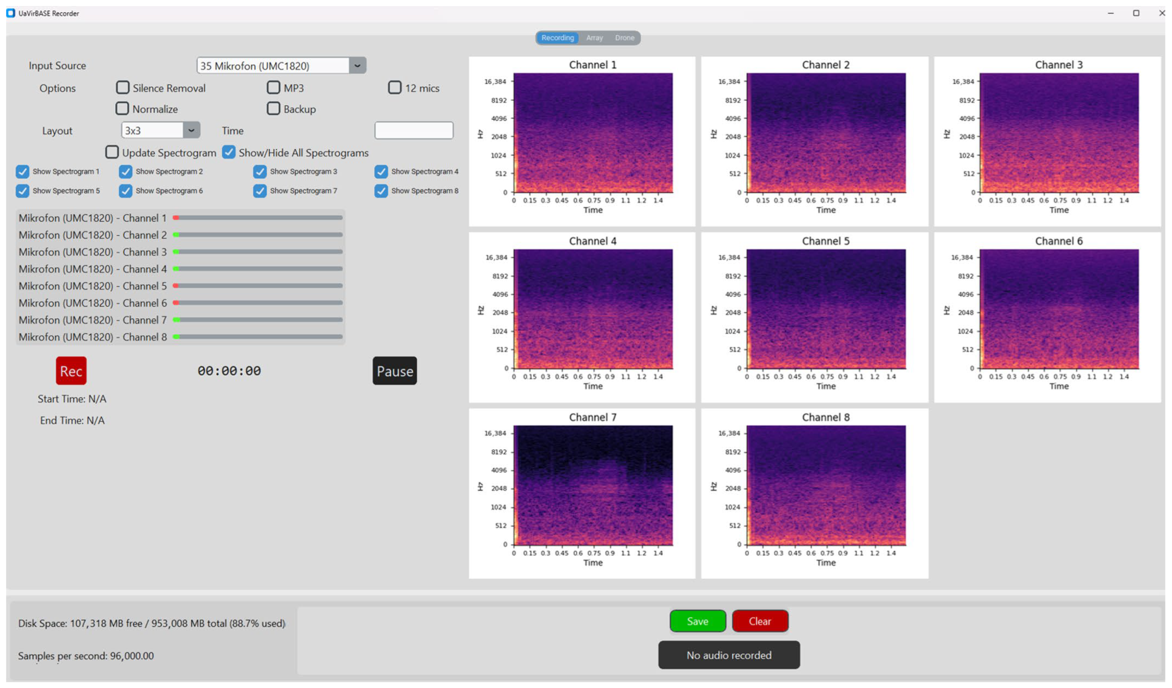
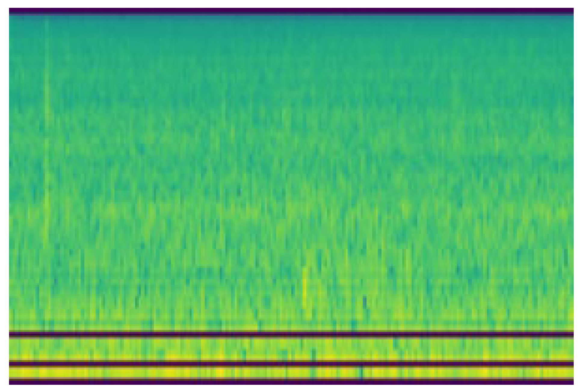
As shown in Figure 7, the interface allows for the simultaneous visualization of live spectrograms for individual audio channels. These spectrograms, displayed in a grid layout, provide immediate insights into the frequency content and temporal dynamics of the captured audio signals. Users can toggle individual spectrograms on or off for focused analysis.

Beyond visualization, the software includes essential functionalities for recording management:

• Silence Removal and Normalization help optimize recordings by removing unnecessary data and ensuring consistent amplitude levels across channels.
• Backup Recording, a critical data redundancy feature, ensures that all recordings are securely saved.
• MP3 support enables audio data to be saved in the MP3 format for reduced file size and storage efficiency. Recordings are saved in the high-quality WAV (Waveform Audio File Format) for maximum fidelity by default. A control panel is used for starting, pausing, and stopping recordings, minimizing operational complexity during experiments.
• To ensure uniformity in the length of audio files across recordings, the time field allows users to specify the duration (in seconds), after which the recording will automatically stop and be saved.

The real-time status bar updates on recording parameters, including the current sampling rate, disk space usage, and recording duration. Moreover, metadata such as start and end times for recordings are displayed, providing an apparent temporal reference that simplifies subsequent data processing. The interface also incorporates straightforward file management through dedicated save and clear buttons.

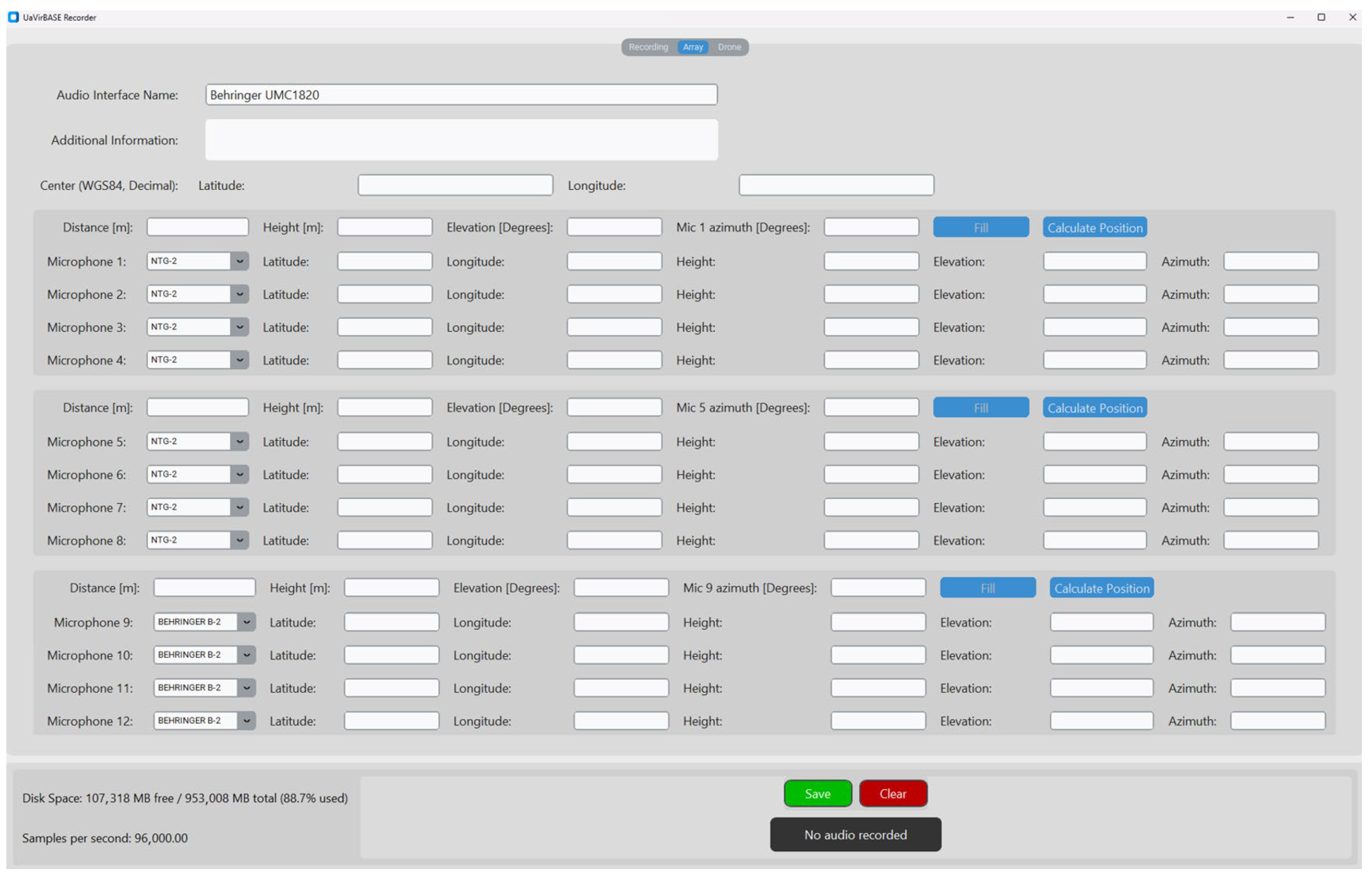
The Array Tab (Figure 8) provides an interface for configuring and managing microphone arrays. This tab’s core feature is the ability to define the spatial configuration of microphones relative to a central reference point. It also allows the selection of core hardware elements, such as audio interfaces and microphones.

One of its key functionalities is the capability to define the array’s reference point through WGS84 coordinates. By entering the latitude and longitude of the central location, users establish a fixed anchor point from which the positions of all microphones are determined.

For each microphone, users can specify several parameters that define its exact position and orientation within the array:

• Distance is the radial distance of the microphone from the center, measured in meters.
• Height is the vertical position of the microphone relative to the ground, also in meters.
• Elevation and azimuth—these parameters define the microphone’s vertical and horizontal angles relative to the center point, ensuring precise orientation and alignment within the array.

Using the provided data, the precise position of each microphone is calculated, taking into account its distance, height, elevation, and azimuth relative to the central reference point. Each microphone is uniquely labeled once the calculations are complete, ensuring clear identification and organization within the array.

Figure 9 depicts a dedicated interface for configuring the sound source. This tab allows us to select whether the recording will capture ambient noise or a drone’s acoustic signature. In the case of drones, users can choose from a predefined list of models, such as DJI Mavic 3 Cine, DJI Mavic 2, or DJI Matrice 300, ensuring compatibility and accurate metadata labeling.

Additionally, the tab enables users to specify whether the drone is static (stationary) or dynamic (moving). The software records the drone’s position relative to the microphone array for static drones. This includes the distance, height, and azimuth (with north defined as 0 degrees). These fields allow for precise spatial configuration, ensuring the recorded data accurately represent real-world conditions.

By combining these features, the Drone Tab simplifies setting up drone-based experiments, providing flexibility and precision in defining the acoustic environment. Whether simulating a stationary noise source or replicating the dynamics of a moving UAV, this tab ensures that the collected data are accurate and reproducible.

2.3. Data Annotation

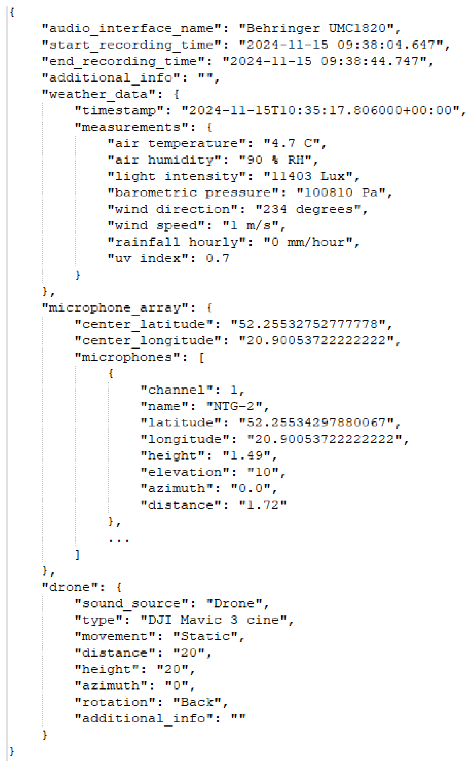
After each recording session, two files were generated: an a.wav file containing the multi-channel audio data and a.json file that stores metadata. The JSON file includes comprehensive information about the recording setup, including environmental conditions, microphone array configuration, and sound source characteristics. The labeling process was fully automated and integrated into the recording system. UAV parameters—such as distance, height, azimuth, and side orientation—were predefined through the recording interface and automatically stored in the JSON file. Microphone positions were established using physical measurements (e.g., tape measure for distance and height and compass for azimuth), and data on the weather were collected in real time via a weather sensor. This setup ensured precise and consistent ground truth labeling without the need for manual annotation. An excerpt of the metadata structure is shown in Figure 10.

Due to its length, the provided structure does not include all microphone labels. However, all microphone labels are listed in the same format, as shown in the example.

3. Experiments

This section provides an in-depth analysis of the created dataset, the architecture and configuration of the deep neural network model, the feature extraction methods utilized, and the results achieved during training. We outline the dataset’s structure, highlight the importance of the selected features, describe the model’s architecture, and discuss the training outcomes supported by relevant metrics and observations. The model was implemented using the PyTorch framework (version 2.6.0+cu126).

3.1. Dataset

The dataset created for this study consists of recordings from two distinct sound sources: ambient noise and UAV sounds. As summarized in

Table 2. Dataset summary.

Sound Source	Number of Recordings	Total Size [GB]	Length [s]
Ambient Noise	4	1.19	416
UAV	128	14.61	5120

, the dataset includes four ambient noise recordings totaling 1.19 GB with a combined duration of 416 s. In contrast, the UAV recordings—captured using a single DJI Mavic 3 Cine drone—are more extensive, with 128 recordings amounting to 14.61 GB and a total length of 5120 s.

In addition to the previously described recordings, we collected 18 audio files totaling 16.15 GB using the Zoom H4essential recorder. These recordings have a total duration of 33,090 s, sampled at a 96 kHz frequency with a 32-bit depth, ensuring high-resolution audio capture.

We performed recordings at varying heights and distances to capture UAV acoustic signatures under controlled conditions. The UAV was positioned and recorded under the following configurations:

• Height: 10 m; distance: 10 m;
• Height: 10 m; distance: 20 m;
• Height: 20 m; distance: 10 m;
• Height: 20 m; distance: 20 m.

At each position, recordings were conducted with an azimuth resolution of 45 degrees, covering eight orientations around the acoustic array.

Furthermore, for each UAV position and orientation, we recorded four separate sessions where the UAV was facing different directions relative to the acoustic measurement system:

• On the left side, towards the acoustic array;
• On the back side, towards the acoustic array;
• On the right side, towards the acoustic array;
• On the front side, towards the acoustic array.

Each recording session lasted 40 s, with 75% of the data (30 s) used for training and the remaining 25% (10 s) used for testing. This setup resulted in 64 files per height–distance combination, 16 files per azimuth angle, and 32 files per UAV orientation.

3.2. Features

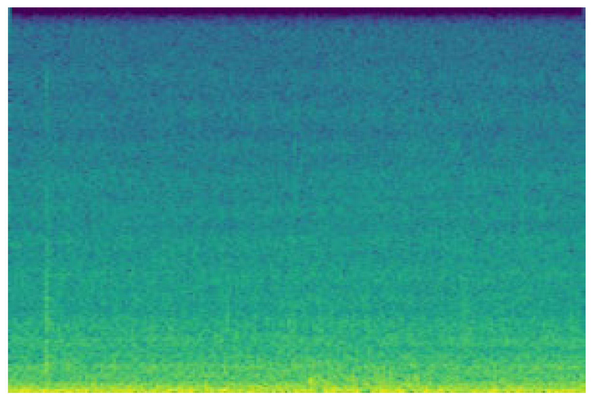
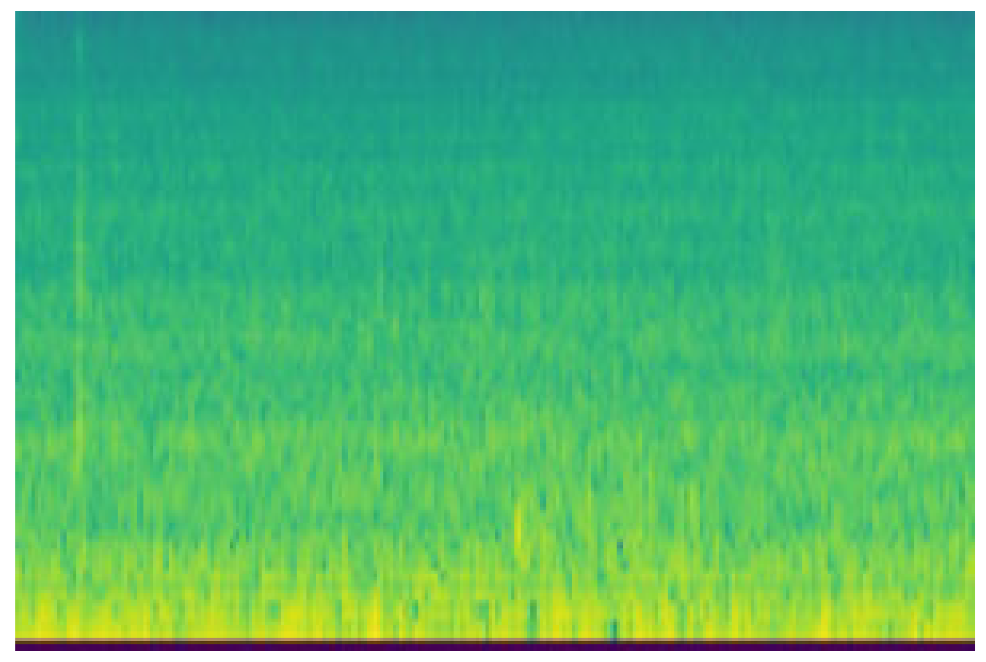
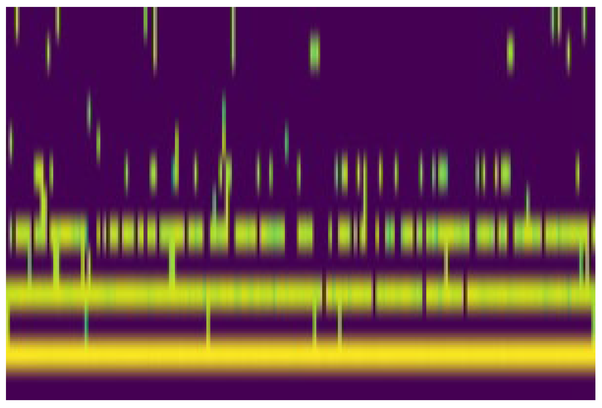
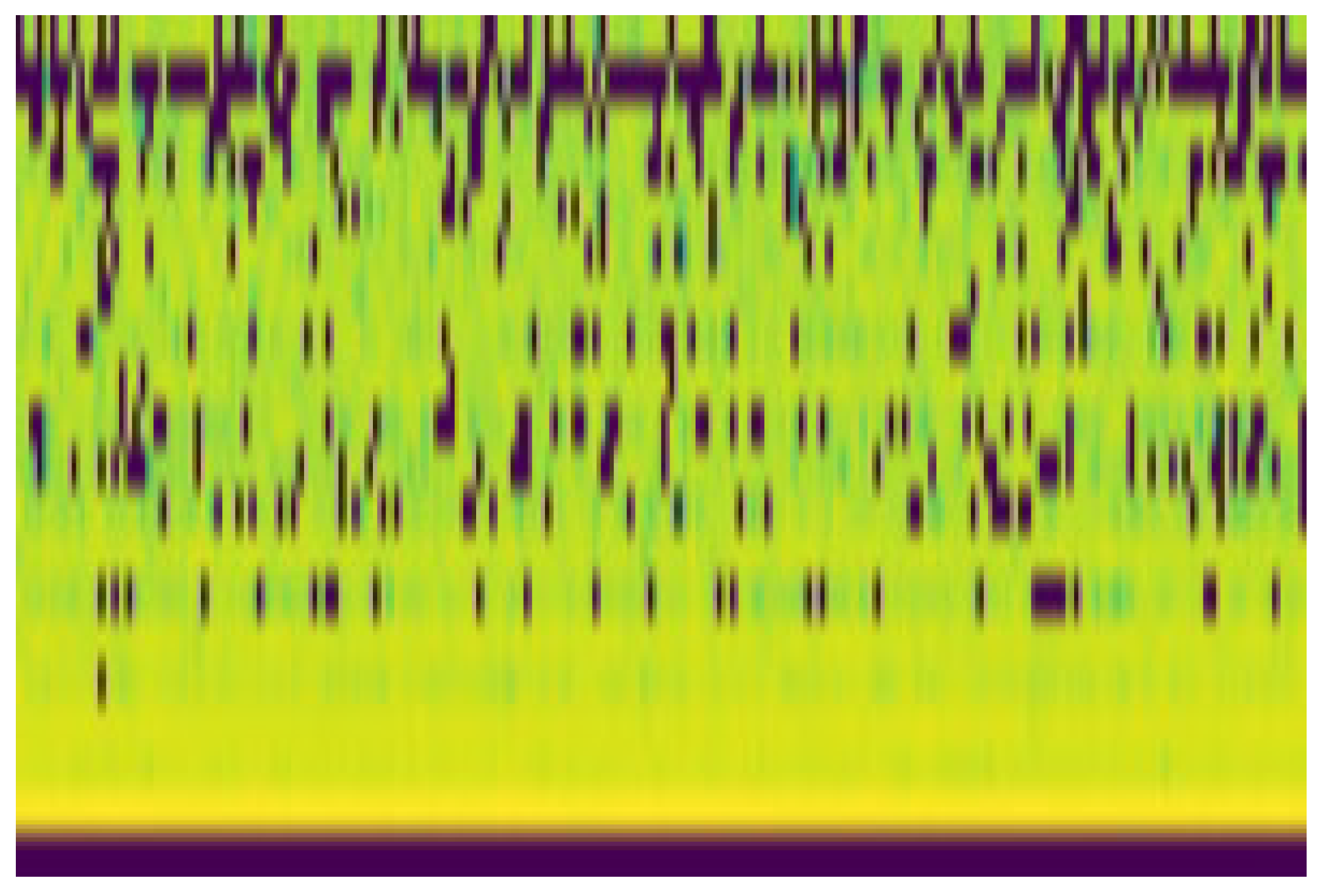
For our experiments, we decided to utilize five distinct audio features: MFCC (Mel-Frequency Cepstrum Coefficient), Mel Spectrogram, STFT (Short-Time Fourier Transform), LFCC (Linear-Frequency Cepstrum Coefficient), and Bark Spectrogram. Each feature was selected based on its unique characteristics and ability to capture specific aspects of audio signals. The model was trained on each feature and configuration for 50 epochs to evaluate its effectiveness.

MFCCs provide a compact representation of the spectral envelope of a signal by mapping it onto the Mel-frequency scale, which approximates the human auditory system’s response. The process involves applying a Fourier Transform, converting to the Mel scale, taking the logarithm, and applying a Discrete Cosine Transform (DCT) to extract a set of coefficients.

A Mel Spectrogram is a time–frequency representation of an audio signal where the frequency axis is transformed to the Mel scale. It is obtained by applying a Short-Time Fourier Transform (STFT) followed by Mel filterbank processing, which smooths the spectrum into perceptually relevant frequency bands.

STFT is a fundamental method for time–frequency analysis, dividing the signal into small overlapping windows and applying the Fourier Transform to each window separately. The result is a spectrogram representing how the signal’s frequency content evolves.

LFCCs are similar to MFCCs but use a linear frequency scale instead of the Mel scale. This allows for a more uniform representation of the spectral content across all frequencies rather than emphasizing lower frequencies, as in MFCCs.

A Bark Spectrogram represents the power of an audio signal in critical bands based on the Bark scale, which approximates how humans perceive differences in frequency. It is computed similarly to a Mel Spectrogram but applies Bark filterbanks instead of Mel filters.

Figure 11, Figure 12, Figure 13, Figure 14 and Figure 15 below illustrate example visualizations of the same audio signal.

3.3. Architecture and Learning Process

Deep learning, particularly convolutional neural networks (CNNs), is well suited for analyzing the time–frequency representations of audio signals, such as spectrograms. In this study, we selected a deep residual CNN due to its ability to effectively learn spatial patterns in 2D acoustic feature maps while preserving gradient flow through skip connections. Compared to traditional machine learning models, CNNs offer superior performance on image-like input data and can automatically extract hierarchical features without manual feature engineering. Residual architectures, in particular, are known for their robustness in training deep networks and preventing vanishing gradients. While this approach requires more computational resources and a larger amount of training data, it provides strong generalization capabilities when sufficient data are available.

The proposed architecture is a deep residual convolutional neural network designed to process and analyze eight input images of (256 × 256) size. It consists of multiple convolutional layers with residual connections, which help efficiently extract hierarchical features while maintaining gradient stability. The network follows a ResNet-inspired design, with skip connections facilitating better feature propagation and mitigating vanishing gradients. Group normalization is applied throughout the network to stabilize activations and accelerate convergence. The model gradually reduces spatial dimensions while increasing the number of feature channels, enabling it to capture local and global patterns effectively. Following feature extraction, a global pooling layer condenses the information, which is then processed by fully connected layers. The final output consists of six continuous values representing different predicted parameters. The use of GELU activation and dropout regularization ensures stability and prevents overfitting. The architecture is shown in Figure 16.

Table 3. The successive layers and output that shape our model.

Layer	Output	Filter	Stride
conv1	32 × 256 × 256	3 × 3@32	1
conv2_x	64 × 128 × 128	3 × 3@64	1, 2
conv3_x	128 × 64 × 64	3 × 3@128	1, 2
conv4_x	192 × 32 × 32	3 × 3@192	1, 2
conv5_x	256 × 16 × 16	3 × 3@256	1, 2
conv6_x	512 × 8 × 8	3 × 3@512	1, 2
conv7_x	512 × 4 × 4	3 × 3@512	1, 2
conv8_x	512 × 4 × 4	3 × 3@512	1
Adaptive avg pool 2d	512	-	-
fc 1	256	-	-
fc 2	6	-	-

below outlines the specifications of each layer, including output dimensions, filter size, and stride.

The training process focuses on optimizing a deep learning model using the Adam optimizer, set with a learning rate of 0.0002 and betas (0.5, 0.9) to ensure stable and efficient convergence. Training is conducted for 50 epochs per configuration, utilizing a batch size of 32, balancing computational efficiency and performance.

Each training iteration follows a structured pipeline: forward propagation, where the model processes input data and generates predictions; loss computation, using the Mean Squared Error to evaluate deviations across six continuous outputs; and backpropagation, where the model updates its weight based on gradients derived from the loss.

To further refine training dynamics, a learning rate scheduler adaptively adjusts the learning rate based on model performance, reducing it when progress slows. This prevents stagnation in optimization and allows for finer weight updates as training progresses.

3.4. Metrics

We utilized two commonly used metrics for evaluating performance—MAE (Mean Absolute Error) and RMSE (Root Mean Squared Error). These metrics were chosen to measure prediction errors in distance, height (in meters), azimuth, and side (in degrees), helping to quantify the accuracy of the model’s estimates for each parameter. MAE calculates the average of the absolute differences between predicted and actual values. In the context of distance and height, this gives a straightforward understanding of how much, on average, the model’s predictions deviate from the actual values in meters. For azimuth and the side, expressed in degrees, MAE tells us how much the predicted angular positions differ on average from the actual angles.

In contrast, RMSE calculates the square root of the average squared differences between predicted and actual values. It is susceptible to larger errors, placing greater emphasis on instances where the model’s predictions significantly deviate from the actual values.

$$MAE={\displaystyle \frac{1}{N}}\sum _{i=1}^N|x_i-x|$$

(1)

$$MSE=\sqrt{{\displaystyle \frac{1}{N}}\sum _{i=1}^N{(x_i-x)}^2}$$

(2)

3.5. Results

The results are labeled from a to d, where each label corresponds to a specific parameter:

• a represents the distance (measured in meters);
• b represents the height (measured in meters);
• c corresponds to the azimuth (measured in degrees);
• d represents the side (also measured in degrees).

To assess the model’s performance, we varied several key parameters. These included the following:

• Frequency sample rate—the rate at which the signal is sampled, which can impact the analysis’s temporal and frequency resolution.
• FFT size—the number of points used in the Fast Fourier Transform determines the resolution of the frequency domain representation.
• Hop length—the number of samples between consecutive frames in time–frequency transformations, affecting both computational efficiency and the trade-off between time and frequency resolution.
• Extra parameters—parameters typical to the feature, e.g., the number of MFC coefficients for MFCC or LFC coefficients for LFCC.

The results for selected audio features are shown in

Table 4. Results for selected features.

Feature	Frequency Sample Rate [kHz]	FFT Size	Hop Length	Extra Parameters	MAE				RMSE
					a	b	c	d	a	b	c	d
MFCC	16	512	256	n_mfcc = 13 n_mels = 64	1.06	1.28	2.15	33.99	1.54	1.75	3.82	58.16
	44.1	1024	512	n_mfcc = 26 n_mels = 128	0.68	0.8	1.3	27.22	0.97	1.13	1.97	50.79
	96	4096	2048	n_mfcc = 40 n_mels = 256	0.57	0.41	1.43	18.77	0.78	0.61	2.4	43.25
Mel Spectrogram	16	512	256	n_mels = 64	0.54	0.41	1.15	13.09	0.76	0.66	1.7	31.45
	44.1	1024	512	n_mels = 128	0.39	0.41	0.91	8.61	0.58	0.55	1.36	26.88
	96	4096	2048	n_mels = 256	0.41	0.43	1.09	8.41	0.64	0.62	1.33	25.62
STFT	16	512	256	-	0.96	1.33	2.85	15.95	1.41	1.89	7.01	37.44
	44.1	1024	512	-	0.58	0.59	1.08	11.08	0.79	0.85	1.92	29.27
	96	4096	2048	-	0.5	0.58	1.34	14.79	0.78	0.82	2.13	36.08
LFCC	16	512	256	n_lfcc = 13	1.1	1.26	2.63	31.66	1.57	1.75	4.79	57.11
	44.1	1024	512	n_lfcc = 26	0.65	0.66	1.39	18.4	0.88	0.89	1.98	39.6
	96	4096	2048	n_lfcc = 40	0.56	0.63	1.6	14.08	0.75	0.84	2.48	33.08
Bark Spectrogram	16	512	256	n_barks = 64	0.41	0.47	1.04	14.04	0.65	0.78	1.54	35.54
	44.1	1024	512	n_barks = 128	0.62	0.59	1.14	10.95	0.87	0.87	1.73	29.53
	96	4096	2048	n_barks = 256	0.45	0.48	1.18	11.18	0.61	0.65	1.74	30.89

.

Building on the results above, the Mel Spectrogram demonstrated the most favorable performance compared to the other feature extraction techniques. Notably, increasing the frequency sample rate from 16 kHz yielded a more significant error reduction compared to increasing the sample rate from 44.1 kHz to 96 kHz. However, it is also evident that raising the frequency sample rate to 96 kHz results in further improvements, particularly in the case of MFCC. This finding suggests that a higher sample rate can provide finer temporal details, contributing to more accurate estimations, especially in the context of certain features like MFCC.

Given these observations, we decided to investigate further how other parameters, including the n_fft, hop length, and the number of Mel coefficients, influence the performance of the Mel Spectrogram. Since it has yielded the best results so far, we chose it as the focus for exploring the impact of these changes. To provide a more comprehensive analysis, we created a table with the results based on the following adjustments:

• Frequency sample rate: 44.1 kHz and 96 kHz.
• FFT size: 1024, 2048 and 4096.
• Hop length: 50% and 75% overlap.
• The number of Mel coefficients: 64, 128, and 256.

By varying these parameters, we aimed to identify their individual and combined effects on the performance of the Mel Spectrogram and further fine-tune the model for improved accuracy in spatial parameter estimations. The results of these experiments are presented in

Table 5. Results for different Mel Spectrogram configurations.

Frequency Sample Rate [kHz]	FFT Size	Hop Length	Mel Coefficients	MAE				RMSE
				a	b	c	d	a	b	c	d
44.1	1024	256	64	0.46	0.49	1.22	12.67	0.6	0.64	1.63	32.67
			128	0.42	0.41	1.09	9.0	0.56	0.57	1.53	26.89
			256	0.53	0.52	1.09	10.51	0.72	0.7	1.6	28.29
		512	64	0.47	0.49	1.23	9.79	0.62	0.68	1.79	27.64
			128	0.46	0.42	1.02	9.59	0.6	0.57	1.34	24.69
			256	0.46	0.48	1.15	10.27	0.63	0.64	1.61	27.57
	2048		64	0.47	0.5	0.98	10.52	0.65	0.68	1.29	28.87
			128	0.48	0.51	1.28	11.63	0.63	0.7	1.65	31.49
			256	0.45	0.39	0.95	10.34	0.6	0.51	1.23	28.34
		1024	64	0.52	0.45	1.12	12.98	0.69	0.62	1.51	32.91
			128	0.44	0.42	1.0	8.77	0.58	0.57	1.38	25.38
			256	0.36	0.3	0.94	9.5	0.49	0.42	1.36	25.77
96		512	64	0.57	0.55	1.16	14.3	0.78	0.78	1.57	33.79
			128	0.53	0.29	1.39	9.29	0.7	0.38	1.62	26.18
			256	0.43	0.6	1.0	10.83	0.62	0.8	1.51	28.63
		1024	64	0.56	0.6	1.39	16.35	0.76	0.8	1.99	30.06
			128	0.47	0.49	1.29	9.18	0.68	0.65	1.82	25.49
			256	0.53	0.56	1.16	11.85	0.74	0.73	1.75	30.17
	4096		64	0.54	0.48	1.29	12.0	0.72	0.64	1.8	31.75
			128	0.38	0.47	0.81	10.24	0.52	0.64	1.06	27.63
			256	0.37	0.47	0.92	9.04	0.5	0.66	1.32	26.47
		2048	64	0.65	0.61	1.27	14.9	0.84	0.9	1.74	34.38
			128	0.46	0.4	0.87	9.48	0.67	0.57	1.27	26.13
			256	0.43	0.45	1.03	9.45	0.63	0.63	1.34	26.56

below.

Analyzing the results presented in the table, it becomes evident that, in most cases, using 64 Mel coefficients resulted in the worst performance. This suggests a lower number of Mel coefficients may not capture sufficient spectral information to achieve optimal results. An interesting trend emerged for parameter a: a hop length overlap of 75% led to better results, indicating that a greater degree of overlap contributed to improved performance. On the other hand, when considering height, the best outcomes were observed with a 50% overlap, suggesting that the impact of the hop length’s overlap may be parameter-dependent.

Another key observation is that parameter d (side) achieved the highest performance when the number of Mel coefficients was set to 128. This implies that, at least for this parameter, a higher number of Mel coefficients provides a more detailed spectral representation, leading to improved results. However, when examining distance, height, and azimuth, no clear trend was identified regarding the impact of the number of Mel coefficients. The results for these parameters do not show a consistent improvement or decline as the number of coefficients changes, making it difficult to draw definitive conclusions.

Additionally, when analyzing the effect of frequency sample, it is not straightforward to determine whether a higher frequency consistently leads to better performance. The results for both frequency values are comparable, indicating that the influence of this factor is less pronounced than other parameters.

The most significant factor affecting the proposed configurations appears to be the number of Mel coefficients. This parameter has the most significant impact on performance, highlighting the importance of selecting an appropriate number of coefficients to maximize the model’s effectiveness. Further analysis could be beneficial in understanding the interaction between Mel coefficients and other parameters and determining the optimal configuration for different use cases.

4. Future Directions

Based on our current work and an analysis of future requirements, we identified several key areas for further development and improvement. The current dataset exhibits limitations in three key spatial dimensions:

• Azimuth Resolution—the localization is presently constrained to a 45° angular increment; thus, we aim to increase angular resolution.
• Altitude Range—the existing recordings cover a limited vertical spectrum (10 and 20 m). We plan to extend this with low- and high-altitude scenarios.
• Radial Distance—the current operational radius from the acoustic head is limited to 20 m. Future trials will focus on extending this range to include greater distances.

Expanding spatial coverage in all three dimensions—along the azimuth, altitude, and radial distance—is expected to improve the precision and robustness of UAV localization. However, increasing the resolution and range also means handling more data and more complex scenarios, which significantly raises processing demands. This can impact real-time performance and require greater computational efficiency. As a result, improvements such as reducing input data size and simplifying model structures will be necessary to maintain accuracy while keeping latency and resource usage within practical limits.

Another identified limitation is the absence of multiple UAV types and overlapping sources in the dataset. At present, our recordings are limited to a single UAV model and single-object scenarios. To address this, we plan to expand our fleet and conduct additional recording sessions using different UAV models individually to increase acoustic diversity. In future stages, we also intend to perform sessions with multiple UAVs operating simultaneously, enabling research into more complex tasks such as sound source separation, interference handling, and multi-target classification.

In parallel with the spatial expansion, we are also working on complementary datasets focused on UAV detection and classification tasks, which will support broader use cases beyond localization. Looking ahead, we plan to develop a dataset involving dynamic UAV movements tracked via GPS to enable future research into real-time acoustic tracking and trajectory estimation. These additions will extend the practical relevance of our work to more complex scenarios involving moving targets and diverse drone behaviors.

Additionally, we are exploring the development of a similar project and dataset tailored for an ad hoc network using a mesh of independent sensors. Such a system poses unique challenges, requiring the design and implementation of new software and hardware solutions distinct from those presented in this study.

As we continue refining our device and dataset, it is evident that creating a large, high quality and comprehensive dataset requires substantial time and resources. The sheer diversity of commercially available UAVs, not to mention custom-built or one-of-a-kind vehicles, makes it impractical for a single team to catalog them all. We are considering publishing our software and hardware as an open-source project to address this challenge. This approach would invite contributions from other interested parties, enabling them to create their own datasets.

5. Conclusions

In this paper, we present a self-created UAV sound database designed for UAV localization, focusing on distance, height, and azimuth and predicting the drone’s side relative to the microphone array. To validate the utility of the dataset, we implemented a deep neural network (DNN) model and demonstrated that the dataset is effective for these tasks. Such a system has practical potential for ground-based UAV monitoring in real-world applications, including airspace surveillance, infrastructure protection, and acoustic detection in areas where visual or RF-based systems are limited.

The results indicate that our model, trained using this dataset, achieves strong performance, with an average MAE of 0.5 m for distance and height. The azimuth error, on average, is around 1 degree, demonstrating the model’s ability to accurately estimate the direction of the sound source. Furthermore, the model reliably predicts the position of the side of the drone, with an average error below 10 degrees, showcasing the ability to classify the drone’s orientation relative to the microphone array. On the other hand, RMSE for distance, height, and azimuth does not vary significantly, indicating stable and consistent predictions for these parameters. However, the RMSE for the side angle is notably higher, suggesting greater variability in these predictions. This implies that while the model can classify the drone’s general orientation well, fine-grained distinctions in its exact side positioning may be more challenging to capture.

Our analysis also reveals that the Mel Spectrogram outperforms other feature extraction methods, such as STFT, LFCC, MFCC, and the Bark Spectrogram, to provide the most accurate results. This suggests that Mel Spectrograms are particularly well-suited for UAV localization tasks involving acoustic data. Additionally, we show that specific parameters, such as the audio frequency sample rate and key feature extraction parameters—like FFT size, hop length, and the number of coefficients—significantly impact the model’s performance. Our experiments show that using very low parameter values in feature extraction leads to a noticeable drop in model performance, likely due to insufficient resolution in the time or frequency domain. Increasing these values improves accuracy, but only up to a certain point. Beyond that, further gains are minimal while computational demands rise sharply. This indicates that selecting moderate parameter settings can offer an effective balance between accuracy and efficiency.

These findings underscore the importance of carefully considering both the dataset and the feature extraction process when designing UAV sound source localization systems. The results suggest that with proper training and parameter tuning, deep learning models can achieve high levels of accuracy in real-world UAV localization tasks.

In conclusion, our study not only introduces a valuable resource in the form of the UAV sound database but also provides insights into effective methodologies for UAV localization using acoustic signals. All the data and code related to this research have been made publicly available under a GitLab repository, ensuring transparency and reproducibility.

Although the current version of UaVirBASE includes data from only one UAV, it presents a fully described and reproducible setup for UAV localization using spatial audio. The dataset is accompanied by detailed metadata, the documentation of the hardware configuration, and a publicly available training code. This will enable others to replicate the setup and develop their own datasets for related research applications.

We believe this research contributes to the advancement of UAV-based localization systems and lays a foundation for future work to improve sound-based localization in complex UAV environments.