Region-of-Interest Extraction Method to Increase Object-Detection Performance in Remote Monitoring System

Abstract

This study proposes an image data preprocessing method to improve the efficiency of transmitting and processing images for object detection in distributed IoT systems such as digital CCTV. The proposed method prepares a background image using Gaussian Mixture-based modeling with a series of continuous images in the video. Then it is used as the reference to be compared with a target image to extract the ROIs by our DSSIM-based area filtering algorithm. The background areas beside the ROIs in the image are filled with a single color—either black or white to reduce data size, or a highly saturated color to improve object detection performance. Our implementation results confirm that the proposed method can considerably reduce the network overhead and the processing time at the server side. From additional experiments, we found that the model’s inference time and accuracy for object detection can be significantly improved when our two new ideas are applied: expanding ROI areas to improve the objectness of each object in the image and filling the background with a highly saturated color.

1. Introduction

Object detection is one of the major areas in computer vision, which identifies the type and location of each object in an image. Using well-trained artificial neural networks for object detection becomes a major trend in this research field, and the advance of Convolutional Neural Networks (CNN) has led to significant performance improvements in accuracy, utilization, etc. Because object detection using CNN requires a lot of computation, it is common to use high-speed processing units such as GPUs. Such requirements would be intensified when various objects need to be detected in real time across multiple images.

A representative example of application of object-detection technology can be an intelligent surveillance camera. If surveillance cameras can detect and report abnormal objects or situations in real time, it will be easier to prevent accidents and to reduce monitoring manpower. Generally, intelligent surveillance systems are designed in a centralized manner to satisfy real-time performance while operating a lot of surveillance cameras simultaneously.

An expected problem when centrally processing object detection for many images is the considerable transmission overhead in the networks and the enormous processing load at the server side. As high-resolution images become common due to recent advances in camera technology, such requirements of the infrastructure are also expected to increase more and more. Therefore, for efficient operation of an intelligent surveillance camera system, to minimize the data transmission and central processing requirements could be a very important challenge.

A motivation of our research is from the expectation that those requirements in the networks and the server side would be reduced if we can select some meaningful areas for processing from the images generated by a surveillance camera such as digital CCTV. In a general object-detection process using a CNN-based model, a window with a constant or variable size searches the area of the image to perform classification. However, CCTV is installed fixedly and the images in captured video share the characteristic of having the same or very similar background. It is expected that this specificity allows object detection to be processed only on areas where changes have occurred compared to a fixed background image, but not on unnecessary areas.

In Section 2, we describe some important existing researches on object detection for CCTV and image quality assessment that are closely related to our research. In Section 3, we propose a new method to extract meaningful target areas for object detection by comparing images. Section 4 presents implementation details and some experimental results to show the usefulness of the proposed method. Finally, Section 5 concludes the paper.

2. Related Research

Most intelligent surveillance systems utilize algorithms based on Regions with CNN features (R-CNN) to perform object detection and dangerous situation recognition with images captured from cameras.

In [1], U. V. Navalgund and P. K proposed a system using the Fast R-CNN model to detect two types of weapons: guns and knives. When the system detects a potential crime situation, it sends an SMS message to a human supervisor to take necessary actions. Liu et al. proposed a video surveillance method for indoor environments based on a well-trained Mask R-CNN model using the Microsoft COCO dataset [2].

In the above methods based on R-CNN, there are several common processes for object detection. First, a regional proposal process is performed to suggest areas where objects are likely to be located. After the regional proposal process, a feature extraction process is followed for the proposed areas. Finally, for each proposed area, object classification or regression to estimate the object’s location is performed. Feature extraction, object classification, and regression have undergone little modification since they are basic processes of the R-CNN model. On the other hand, there have been various approaches to improve the regional proposal process.

The early R-CNN method used the selective search algorithm [3]. The algorithm uses the brightness of pixels to create components and group them to find regions [4]. This method has the disadvantage that requires a long time for many calculations, such as having all found regions pass a CNN model and running a Support Vector Machine (SVM) for each class for each result.

Two improved methods, Fast R-CNN and Faster R-CNN, applied the Regional Proposal Network (RPN) instead of the selective search algorithm [5,6]. Figure 1 shows the architecture for Faster R-CNN to perform object detection.

In Figure 1, the feature map extracted from the image is processed through a regional proposal network and regions are proposed. The feature map is then ROI pooled according to the proposed regions and classified by regions in the classifier. Because the RPN shares a network with the backbone, it can improve operational efficiency by omitting redundant training. Comparison results using the VGG16 backbone network showed that the time required for the regional proposal process was significantly reduced by the application of the RPN. This is evaluated as having advanced to a level where the real-time object detection is possible [5].

More recently, one-stage detectors have emerged to facilitate real-time inference in practical systems. Unlike their two-stage counterparts, these detectors perform regional proposal and classification simultaneously, eliminating the need for a separate Region Proposal Network (RPN). DETR and YOLO (You Only Look Once) represent prominent examples of this one-stage detection paradigm [7,8,9,10].

DETR (Detection Transformer) introduces an innovative approach by applying the Transformer architecture to computer vision tasks, departing from traditional CNN-based object detection methodologies. This model reconceptualizes object detection as a direct set prediction problem, establishing an end-to-end framework that circumvents complex post-processing operations such as anchor generation or non-maximum suppression (NMS). By harnessing the self-attention mechanism that has proven highly effective in natural language processing, DETR capably models global relationships between objects within images [8]. However, this approach demonstrates reduced accuracy when detecting smaller objects [11].

YOLO is a one-stage object-detection algorithm where a unified network simultaneously predicts both object locations and classes through a single forward pass of an image. This integrated approach delivers high inference speeds suitable for real-time processing while progressively enhancing the balance between accuracy and efficiency across successive iterations. YOLOv8 offers remarkable computational efficiency with a streamlined architecture suitable for edge device deployment [12]. Despite these advantages, systematic evaluations reveal that its performance degrades in scenarios featuring high visual complexity when compared to two-stage detection frameworks.

There have been some approaches to perform regional proposals without using a pre-trained model such as the RPN. For example, in the research field of Abandoned Object Detection (AOD) using surveillance cameras [13], those approaches attempt foreground segmentation using pixel color differences or image features. Methods widely used for this purpose are Mixture of Gaussian [14,15,16] and Kernel Density Estimation [17]. The Mixture of Gaussian method is designed to adapt to changes indoor lighting, and the Kernel Destiny Estimation method is designed to respond sensitively to moving objects. The two methods differ significantly in computational cost [18]. For Mixture of Gaussian, we only store the parameters of a few Gaussian components for each pixel position and evaluate each component on update. Kernel Density Estimation, on the other hand, computes the distance between the pixel values of all stored frames. This difference in computation is something to be aware of when real time is required.

With these methods, since comparison of colors is performed for each pixel, there is a drawback that an object cannot be detected if it has a color similar to the background. In this paper, to address this shortcoming, we propose a method to use Structural Similarity Index Measure (SSIM) instead of pixel-by-pixel comparison [19,20]. This enables the proposed method to consider not only color differences in each pixel but structural differences based on window-by-window comparison.

3. Proposed Method

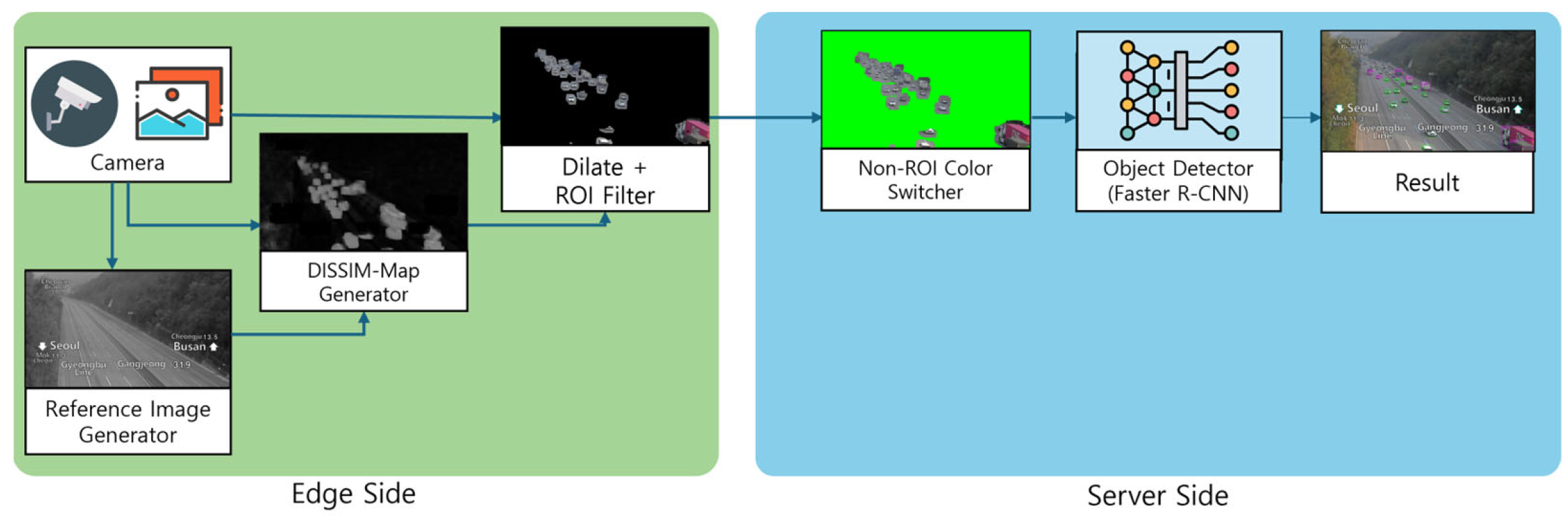
3.1. Method Overview

An important feature of the proposed method is to reduce the load on the server side by extracting and transmitting only Regions of Interest (ROI) through preprocessing of images captured in the edge systems (i.e., surveillance cameras). Figure 2 illustrates the overall process from capturing camera images to object-detection results in the proposed method.

As shown in Figure 2, our proposed method is implemented at both the edge and the server. The traditional method is server-side, receiving images directly from the camera, which places a heavy load on the server. The proposed method removes the background region from the edge side where the camera is located and sends the image in a low-bandwidth format. For this purpose, the Reference Image generator, DSSIM-MAP generator, and RO filter are additionally located on the edge side. On the server side, an additional Background Color Switcher module is deployed to receive images and exchange background colors.

3.2. Reference Image Generator

The Reference Image Generator generates a reference image using multiple images received from a camera. A reference image is a kind of background image, which is constructed through observing colors that show little change over a long period of time. This reference image is used to detect areas where changes have occurred by comparing it with camera images captured in real time. In the real environment, it is not easy to obtain a background image that removes all objects that are likely to change in the future. In our research, to get a more accurate reference image, we adopt a stochastic method that selects color values appearing frequently in the background. Algorithm 1 illustrates the procedure for generating the reference image using Gaussian Mixture modeling.

Algorithm 1: Background Extraction using Gaussian Mixture Modeling

Input: video—input video sequence

Parameters: width—width of video frame

height—height of video frame

channels—number of color channels in video frame

numClusters—number of Gaussian clusters (default: 2)

Output: backgroundImage—static background reference image

procedure ExtractBackground(video)

stackedFramesframes ← Stack(ExtractFramesFromVideo(video))

backgroundImage ← InitializeImage(width, height, channels)

for x = 0 to width-1 do

for y = 0 to height-1 do

for c = 0 to channels-1 do

pixelIntensities[] ← extract intensities(stackedFrames, x, y, c)

clusters[] ← fit GaussianMixtureModel(pixelIntensities, numClusters = 2)

dominantCluster ← get most weighted cluster(clusters)

backgroundImage[x, y, c] ← dominantCluster.mean

return backgroundImage

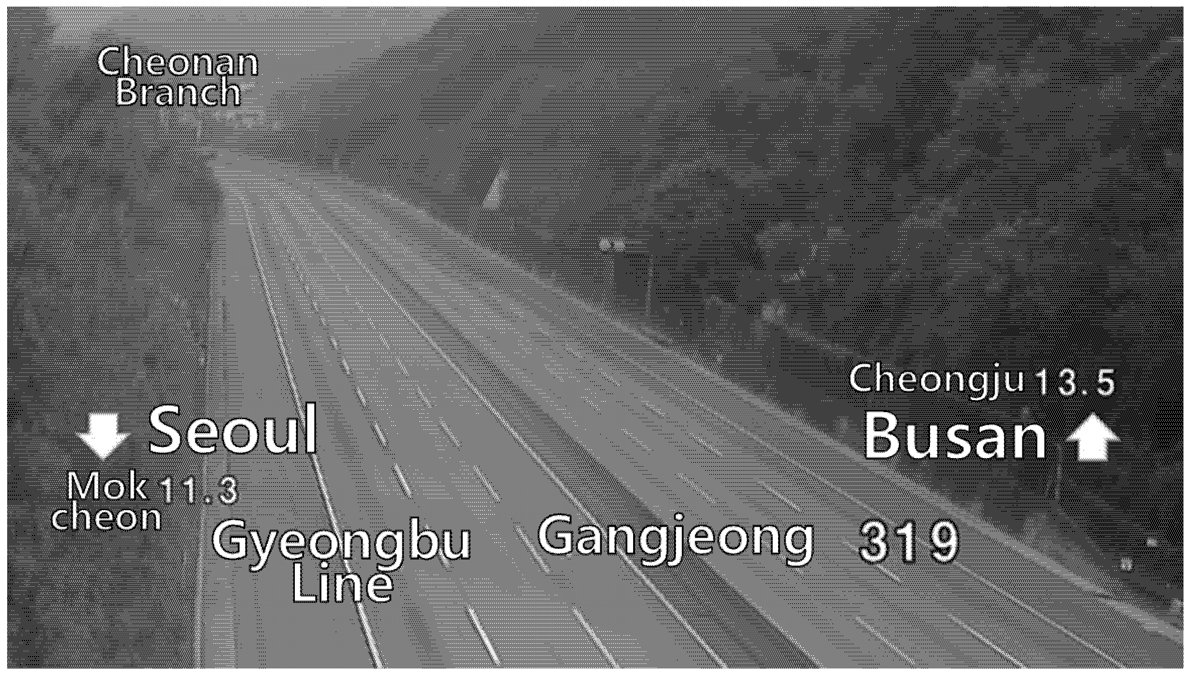
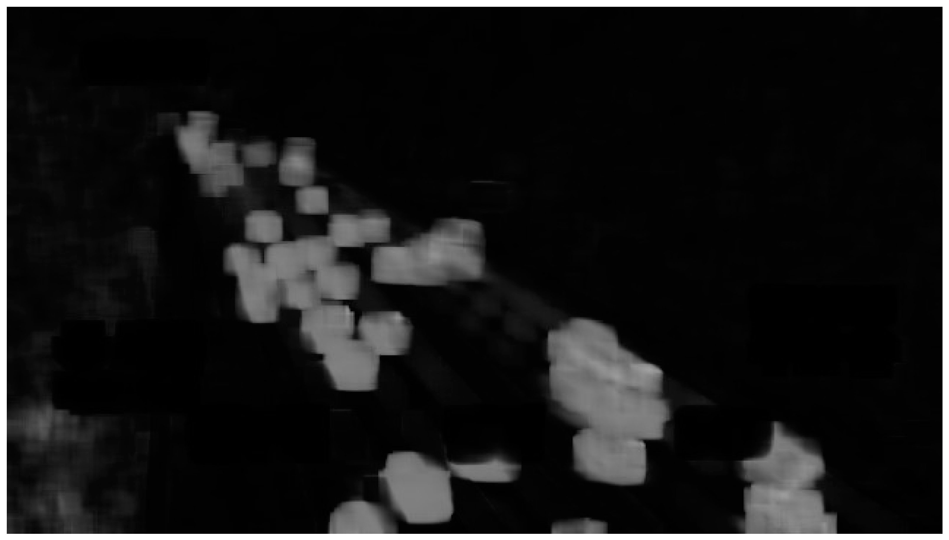
3.3. DSSIM-Map Generator

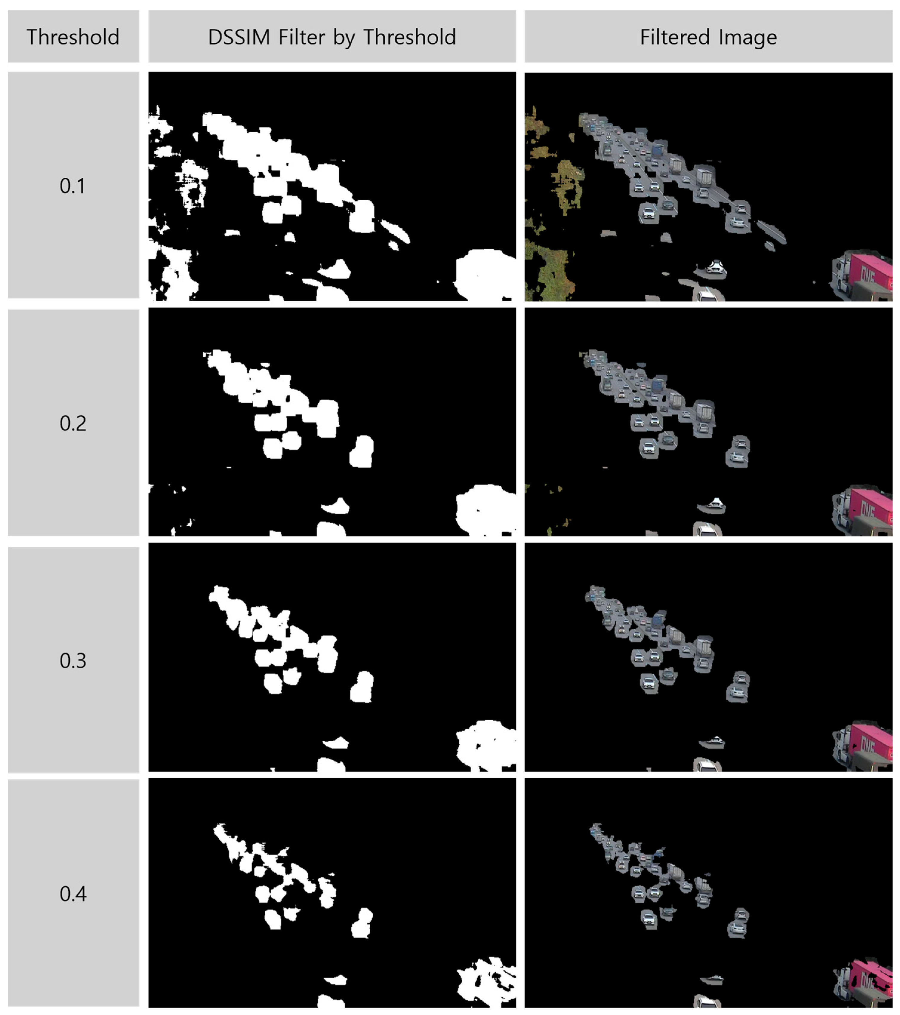
DSSIM-MAP is a map of structural dissimilarity, which measured how much the reference image x and the comparison image y are different over a certain window. Only with simple pixel comparison to measure dissimilarity, if the background and an object have similar colors, it is difficult to recognize the object as differences. Another difficulty is that cameras installed outdoors may suffer from shaking, and in this case, applying the color difference method may result in sensitive responses.

To resolve these problems, our research applies DSSIM-MAP, which is based on SSIM-MAP. A SSIM-MAP is a measured result of structural similarity of two regions through considering the color average and color variance [21]. The general equation to calculate SSIM is as Equation (1).

$$\mathrm{SSIM}\left(x,y\right)={\displaystyle \frac{\left(2{\mu }_x{\mu }_y+C_1\right)\left(2{\sigma }_{xy}+C_2\right)}{\left({\mu }_x^2+{\mu }_y^2+C_1\right)\left({\sigma }_x^2+{\sigma }_y^2+C_2\right)}}$$

(1)

In Equation (1), ${\mu }_x$ and ${\mu }_y$ are the average of the x-area and the y-area, respectively. ${\sigma }_x^2$ and ${\sigma }_y^2$ represent the variance of pixel colors in those two areas, respectively. And ${\sigma }_{xy}$ is the standard deviation of the color of those two areas. $C_1$ and $C_2$ are constants to stabilise the denominator. These values can be calculated using Equation (2):

$$C_i={\left(K_i\times L\right)}^2$$

(2)

In Equation (2), the value of $C_1$ is typically 0.01 and the value of $C_2$ is 0.03. $L$ is the datarange of pixel. In this research we used 255 for $L$.

The equation to calculate DSSIM is as Equation (3) [19,20].

$$\mathrm{D}\mathrm{S}\mathrm{S}\mathrm{I}\mathrm{M}(x,y)={\displaystyle \frac{1-\mathrm{S}\mathrm{S}\mathrm{I}\mathrm{M}(x,y)}{2}}$$

(3)

As presented in the above equations, DSSIM has the opposite direction to SSIM and has a range of values from 0 to 1.0. A window size used to generate a DSSIM-MAP decides the size of the reference area to be compared. In our study, the window size was set to 7 pixels. The DSSIM-MAP Generator produces outputs through three steps: grayscaling, image reduction, and DSSIM calculation.

First, since SSIM and DSSIM are indicators designed based on grayscale images, the average of each color channel in the target image is calculated and grayscaled. Second, the image size is reduced to decrease the amount of calculation required for DSSIM-MAP generation. This is necessary for real-time processing in embedded devices such as surveillance cameras without high-performance GPU. Third, a SSIM-MAP is generated and converted to a DSSIM-MAP. Additionally, morphology calculation is performed on DSSIM-MAP to remove noise and make an object distinct. The noise can be removed by performing opening and closing operations, and the object area can be set sufficiently by erosion or dilate operations.

3.4. ROI Filter

The ROI Filter is used to extract ROI areas by filtering values of the DSSIM-MAP with a certain threshold value. Thus, some areas with higher DSSIM-MAP values than the threshold value are selected as ROI areas in the image.

Since the DSSIM-MAP has been calculated from the size-reduced image, those ROI areas should be expanded to suitable sizes for the original image size. Then all pixels of non-ROI areas in the original image are substituted in a single color (i.e., black). This enables the image codec to compress images with higher compression ratios so that the network burden is reduced to transport those images to the remote server.

3.5. Non-ROI Color Switcher

Images received from the Edge side have their non-ROI areas colored specifically to increase compression rates. The non-ROI Color Switcher replaces these non-ROI areas with colors that rarely occur in natural environments. This process yields higher object-detection performance compared to processing the received images in their original state.

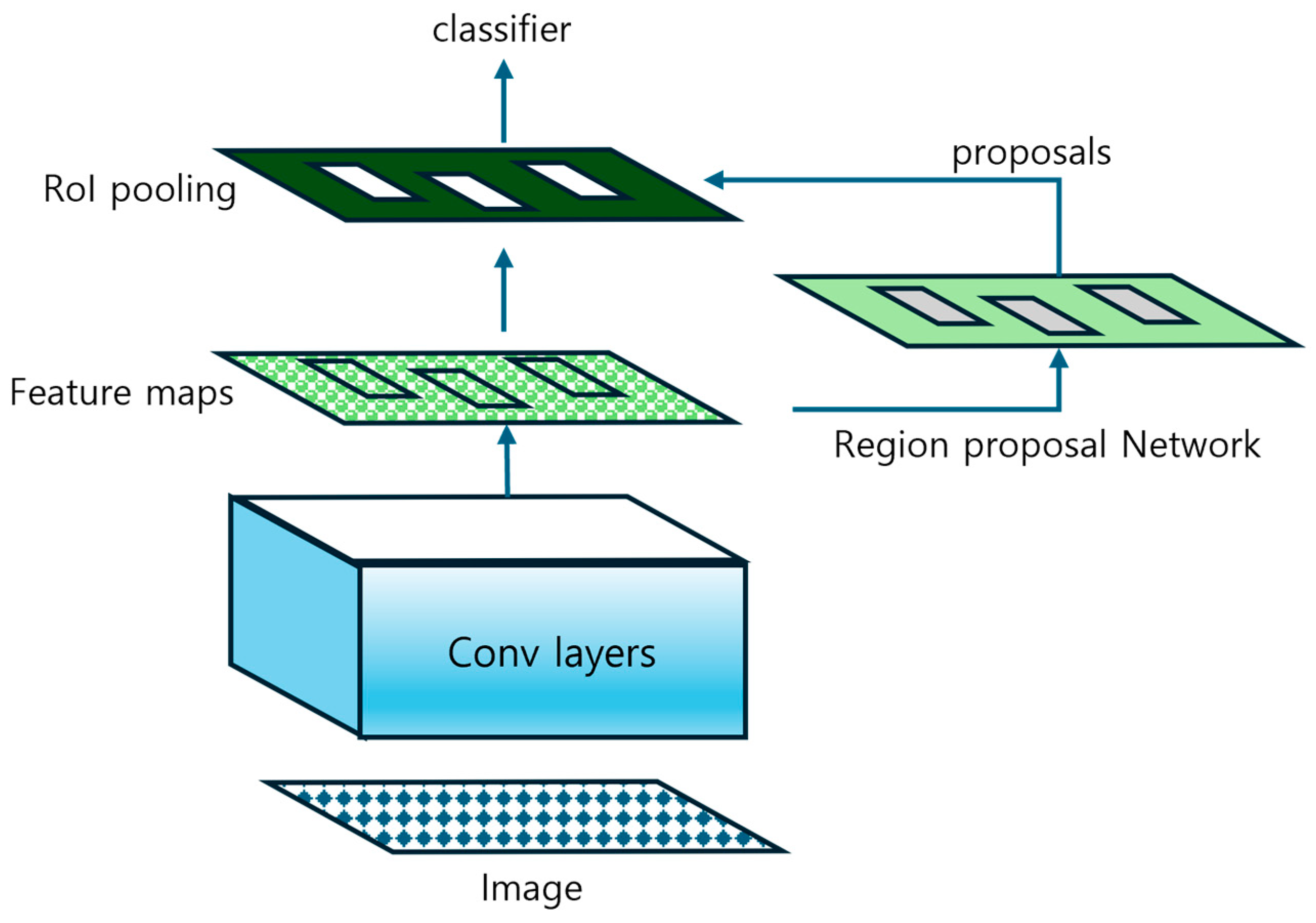
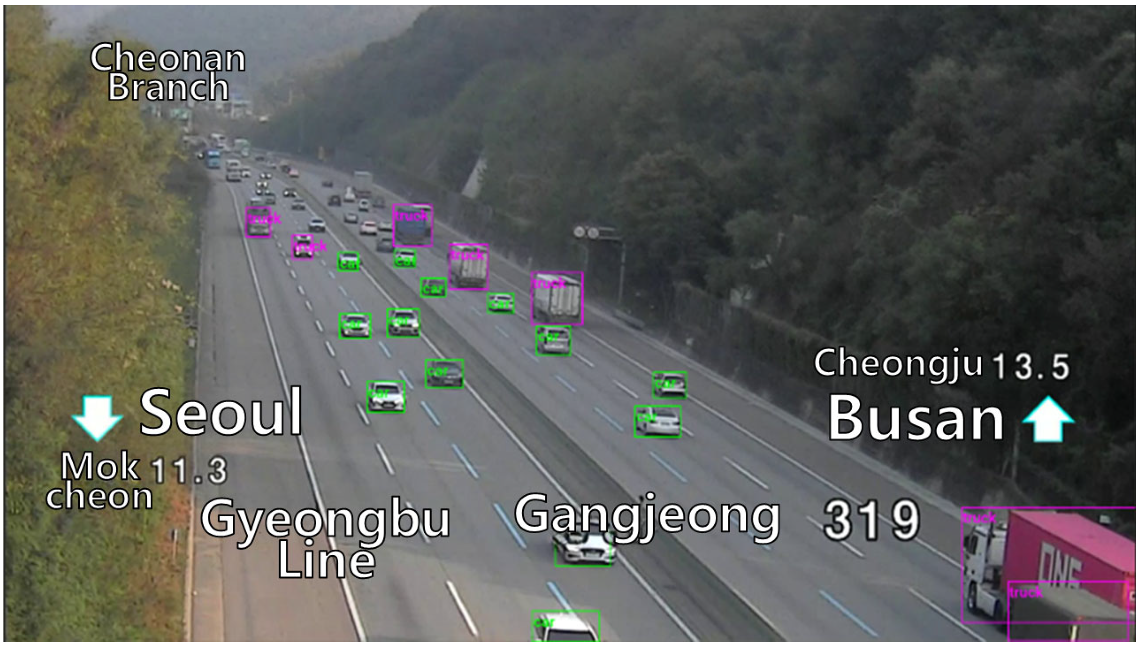
3.6. Object Detector

The Object Detector in the server-side receives ROI-focused images that all non-ROI areas have been painted over with a single color by ROI filtering in the previous step. Because no image features can be found from such single-color areas, those areas are ignored at the ‘regional proposal’ process of general two-stage object-detector models. In Section 4, we present which object detector model is used for our study and the training details.

4. Implementation

4.1. Experiment Environment

4.1.1. Datasets

The dataset used for this study is “The CCTV traffic images (in the highways) for solving traffic problems” provided by AI Hub [22]. This dataset was constructed by sampling every minute the CCTV images monitoring highways in South Korea. The dataset consists of 21,302 images for model training and 2627 images for validation. The size of an image is 1920 × 1080 pixels. Each image shows a two-way road with multiple carriageways, and the number of vehicles in the image is provided as an annotation. The annotation format is CVAT image 1.1, and the bounding boxes of vehicles in the image are given with labels such as ‘car’, ‘truck’ and ‘bus’. The site providing this data reported that mAP@IoU 0.5 achieved 68.2% when object detection was performed using YOLO v4 [22].

Figure 3 illustrates an example image of training data, which its annotation has been visualized.

As shown in Figure 3, the dataset content depicts highway scenarios, with moving vehicles labeled in bounding box format. Additionally, there are background elements that move or sway, such as trees, which could potentially generate noise during the DSSIM-MAP creation process.

4.1.2. Experimental Environment

The experiments have been conducted to evaluate the various performance metrics at the edge side and the server side, respectively.

Table 1. Hardware specification.

Side	Component	Specifications
Edge Side	OS	Raspberry Pi OS
	CPU	Cortex-A76 CPU
	GPU	VideoCore VII GPU
	RAM	LPDDR4X 8GB
Cloud Side	OS	Windows 11
	CPU	Intel(R) Core(TM) i7-13700K
	GPU	Nvidia RTX4090
	RAM	DDR5 32 GB

shows the hardware specification of devices used for our experiments.

4.2. Edge Side

4.2.1. Reference Image Generator

To produce a reference image, the original image was first converted with grayscale and then the background modeling introduced in Section 3 was performed. To do this, the Gaussian Mixture-based background extraction of OpenCV was used [23]. To make one background image, a series of previous 100 input images were referred and the threshold value was set to 16. Figure 4 illustrates a result of the Reference Image Generator.

Compared to Figure 3, Figure 4 shows that moving objects such as vehicles have been removed. This result occurs because the reference image generator applies a statistical model based on Gaussian distribution, selecting representative colors that show temporal consistency across multiple frames. At each pixel location, the color value that appears with the highest frequency is determined as the background, which becomes a reference model that effectively segments areas of moving objects when compared with new input images.

4.2.2. DSSIM Generator

The DSSIM Generator produces a SSIM-MAP with Equation (1) and then converts it to a DSSIM-MAP with Equation (2). Since there is a weakness that much time is required to calculate a SSIM-MAP, its calculation was performed using multi-processing [24]. Additionally, to estimate the proper image size for real-time calculation of an SSIM-MAP, we measured the calculation times of five cases in image resolution: 1920 × 1080, 1280 × 720, 960 × 540, 800 × 450, and 640 × 360.

Table 2. SSIM-MAP Processing Time by Resized Image Resolution in Raspberry Pi 5.

Image Resolution	Processing Time (ms)
1920 × 1080	269.59
1280 × 720	112.68
960 × 540	56.24
800 × 450	37.12
640 × 360	23.37

shows the average processing times when two different images are calculated for 100 times on Raspberry 5, respectively.

As shown in the table, the average time to generate SSIM-MAPs decreases as the resolution of source images becomes smaller. For the original CCTV images with the resolution of 1920 × 1080, the average processing time to generate a SSIM-MAP appeared to be 269 ms. This means our system only handles around 3.7 frames per second. It is not satisfactory when considering that the general CCTV video has a rate of 30 frames per second.

On the other hand, for images with a reduced resolution of 640 × 360, the average processing time decreased to 23 ms and around 42.8 frames can be calculated for a second. Thus, in our experimental environment, 640 × 360 was selected for the appropriate resolution to generate SSIM-MAPs in real time.

Accordingly, each SSIM-MAP was transformed to a DSSIM-MAP by Equation (3) described in Section 3. Figure 5 shows an image painted by translating 0.0~1.0 scale values of a sample DSSIM-MAP to 0~255 scale values.

In Figure 5, a brighter area represents an area with higher DSSIM values. Therefore, bright areas can be interpreted as detected differences from the background, while dark areas correspond to the background and can be considered as having lower value as regions of interest.

4.2.3. ROI Filter

For the next step, each DSSIM-MAP should be expanded to the original image size (i.e., 1920 × 1080). Then the color of background can be removed with a proper threshold for values of the DSSIM-MAP. Figure 6 presents the images with the background removed with threshold values of 0.1~0.4. The left side shows grayscale images, and the right side shows images with original colors.

In Figure 6, we can observe that the vehicle areas in the image become narrower as the threshold value increases. When a lower threshold is configured, some areas were misunderstood as vehicle areas so that the image includes faulty ROIs, which cause unnecessary overhead in the network and the server side.

4.2.4. Video Transmission

A CCTV edge device generally produces video in the H.264 standard format to deliver it to the server side. Most video or image encoding algorithms can achieve high compression performance when a lot of continuous and repetitive color pixels exist within an image or between adjacent images in the video stream. Thus, to replace the background in the original CCTV video with a single color allows us to increase the compression ratio dramatically.

For the experiment, we prepared H.264 video with the rate of 30 frames per second from 240 images included in the dataset. The size of the original video is 60,746 KB. The video file size varies as the DSSIM threshold value is set differently: 59,703 KB for the threshold 0.1, 43,549 KB for 0.2, 32,969 KB for 0.3, and 25,824 KB for 0.4, respectively.

Figure 7 shows the change in bitrate per second when those videos were actually streamed over the network.

In Figure 7, higher DSSIM threshold values show lower bitrates, while lower DSSIM threshold values result in higher bitrates. Notably, when the DSSIM threshold value is 0.2, we can observe a momentary increase in DSSIM values around the 4-s mark of the video. This occurred because camera shake in the video caused elevated DSSIM values across the entire frame.

4.3. Server Side

4.3.1. Model

For the object detection in our implementation, we used a self-trained Faster R-CNN model with a ResNet-50-FPN backbone [25]. Training of the model was performed with the AdamW optimizer [26]. Figure 8 shows the measurement results of losses during model training.

The loss became lowest when the 33rd epoch had been completed. Since the loss increased again after that, we finished early training of the model. When the trained model was evaluated with validation data, the mean average precision (mAP) appeared to be around 72.09%, which indicates a proper training level [27].

4.3.2. Inference Time

We measured inference times of our self-trained model for the ROI-filtered video based on DSSIM values. With an object-detection model based on the Region Proposal Network (RPN), the RPN score threshold can be set to configure the objectness level to select regions in advance to be suggested to the object classification stage [5,25]. In a fast r-cnn fpn v2 model, the default RPN score threshold is 0.05. In our study, we compared two scenarios that the RPN score threshold was set to 0.0 and 0.05 while the DSSIM threshold value varies from 0.0 to 0.4. Figure 9 shows the inference times taken in those two scenarios.

In Figure 9, looking at the results, the average inference time per frame was around 27.652 ms when both DSSIM threshold and RPN score threshold were set to 0.0. The inference time continuously decreased as the DSSIM threshold was set higher.

To apply the RPN score threshold also can reduce the inference time, as shown in the results. But the enhancement did not change significantly depending on how the RPN score threshold was set. In our experiment, the inference time scarcely changed while we gradually increased the RPN score threshold from 0.1 to 0.5. Thus, we presented the results only when the RPN score threshold was set to 0.05, which is the default value.

When the DSSIM threshold exceeded 0.3, the case only with the DSSIM threshold required less inference time than the case only with the RPN score threshold. This implies that the DSSIM filtering may affect more the inference time than the RPM score filtering.

4.3.3. Model Performance

To evaluate the inference performance of our model with different threshold levels, we calculated the precision, recall and F1 score for each object class in the image: bus, car and truck. Then we also calculated the mean average precision (mAP) for different threshold levels.

Table 3. Inference Performance with different DSSIM threshold levels.

DSSIM Threshold	Class	Precision	Recall	F1	mAP
Original	Bus	0.54	0.86	0.67	76.32
	Car	0.54	0.91	0.68
	Truck	0.45	0.95	0.61
DSSIM >0.1	Bus	0.49	0.80	0.61	66.09
	Car	0.51	0.82	0.63
	Truck	0.47	0.87	0.61
DSSIM >0.2	Bus	0.52	0.73	0.61	56.92
	Car	0.52	0.70	0.60
	Truck	0.52	0.74	0.62
DSSIM >0.3	Bus	0.59	0.64	0.62	40.14
	Car	0.52	0.50	0.51
	Truck	0.50	0.48	0.49
DSSIM >0.4	Bus	0.67	0.23	0.35	15.56
	Car	0.56	0.19	0.28
	Truck	0.41	0.25	0.31

presents those calculation results.

As shown in Table 3, the precision, recall, F1 score, and mAP values decreased as the higher DSSIM threshold was applied. These results were obtained using a Faster R-CNN model provided by TorchVision 0.22 (accessed on 29 December 2024) [25], establishing a performance baseline against which we can demonstrate the enhancements achieved through our object-clarification method described in the following sections. When the threshold was greater than 0.3, the F1 scores for three object classes appeared quite different to one another. Especially the recall and F1 score of ‘car’ class was affected more than those of bus and truck classes as the threshold increased. We can analyze that it is because the strong filtering with high threshold values damaged some of each object area in the image and the smaller class, such as car, was suffered more than the other classes.

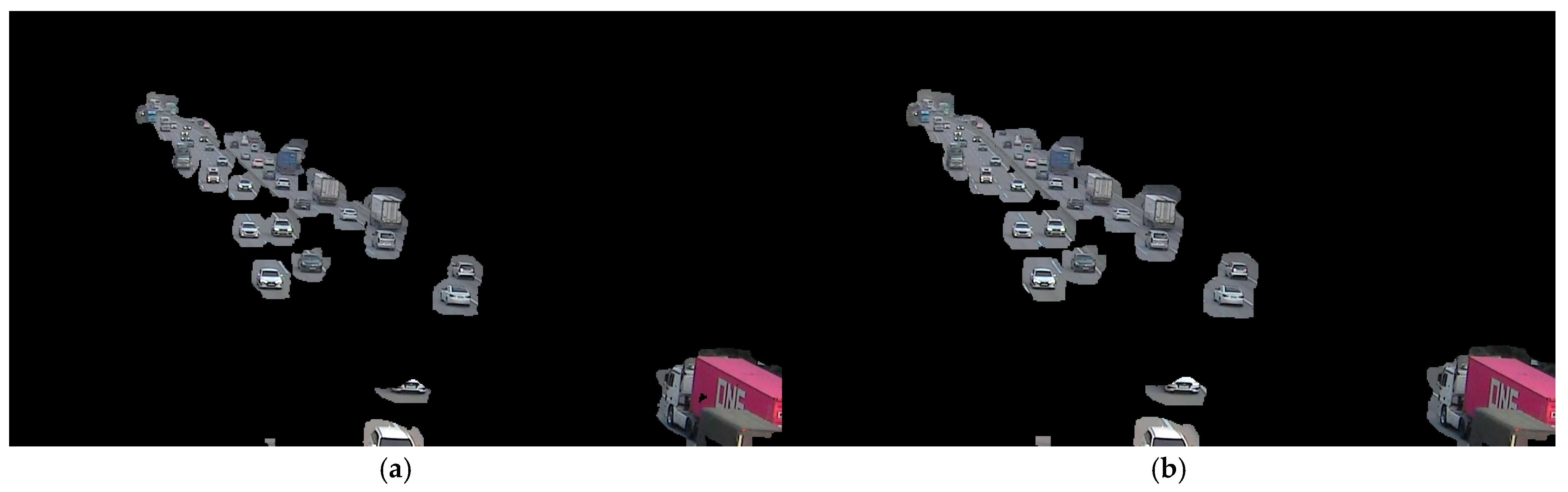
4.4. Objectness Clarification Process

4.4.1. Method to Enhance Objectness

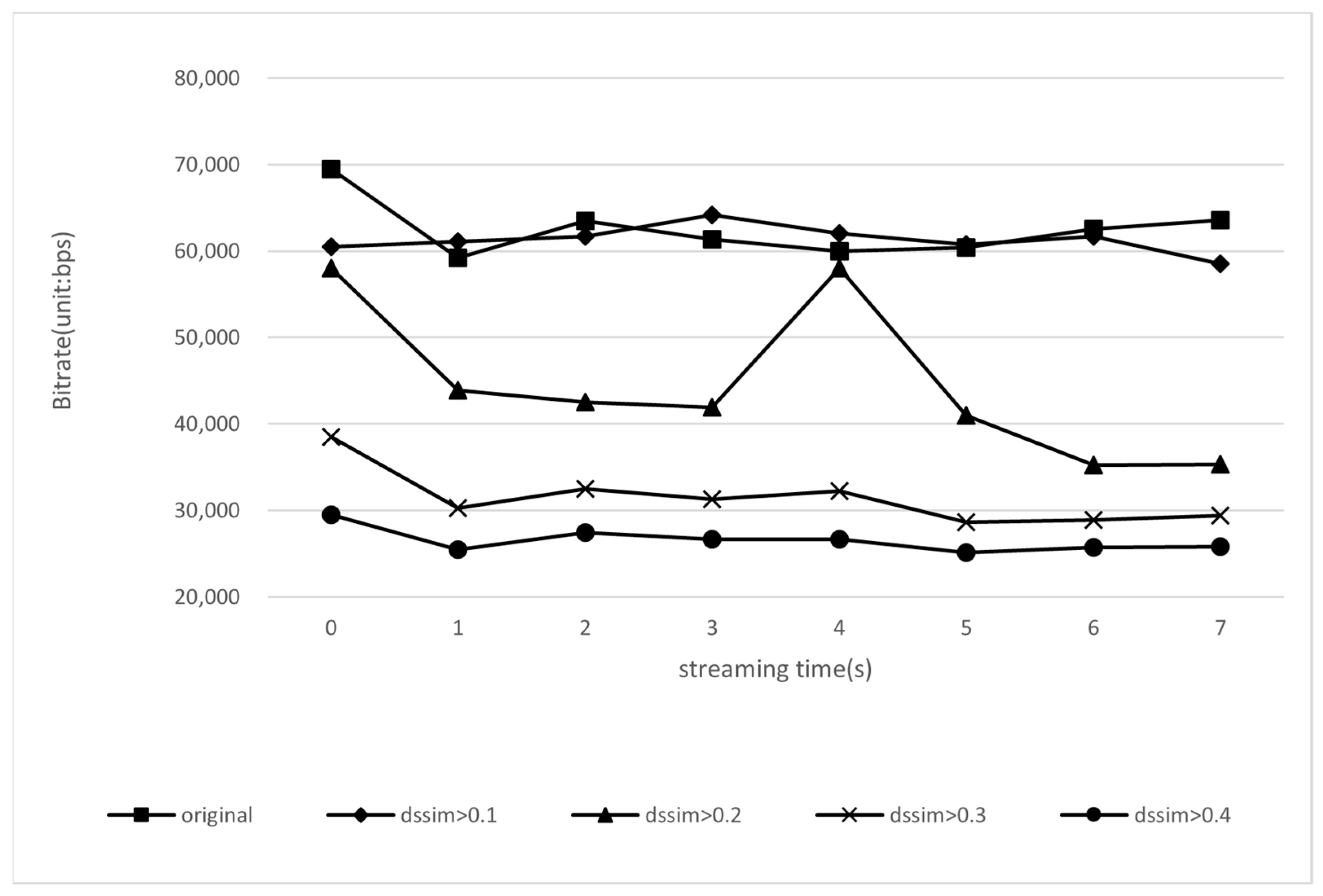
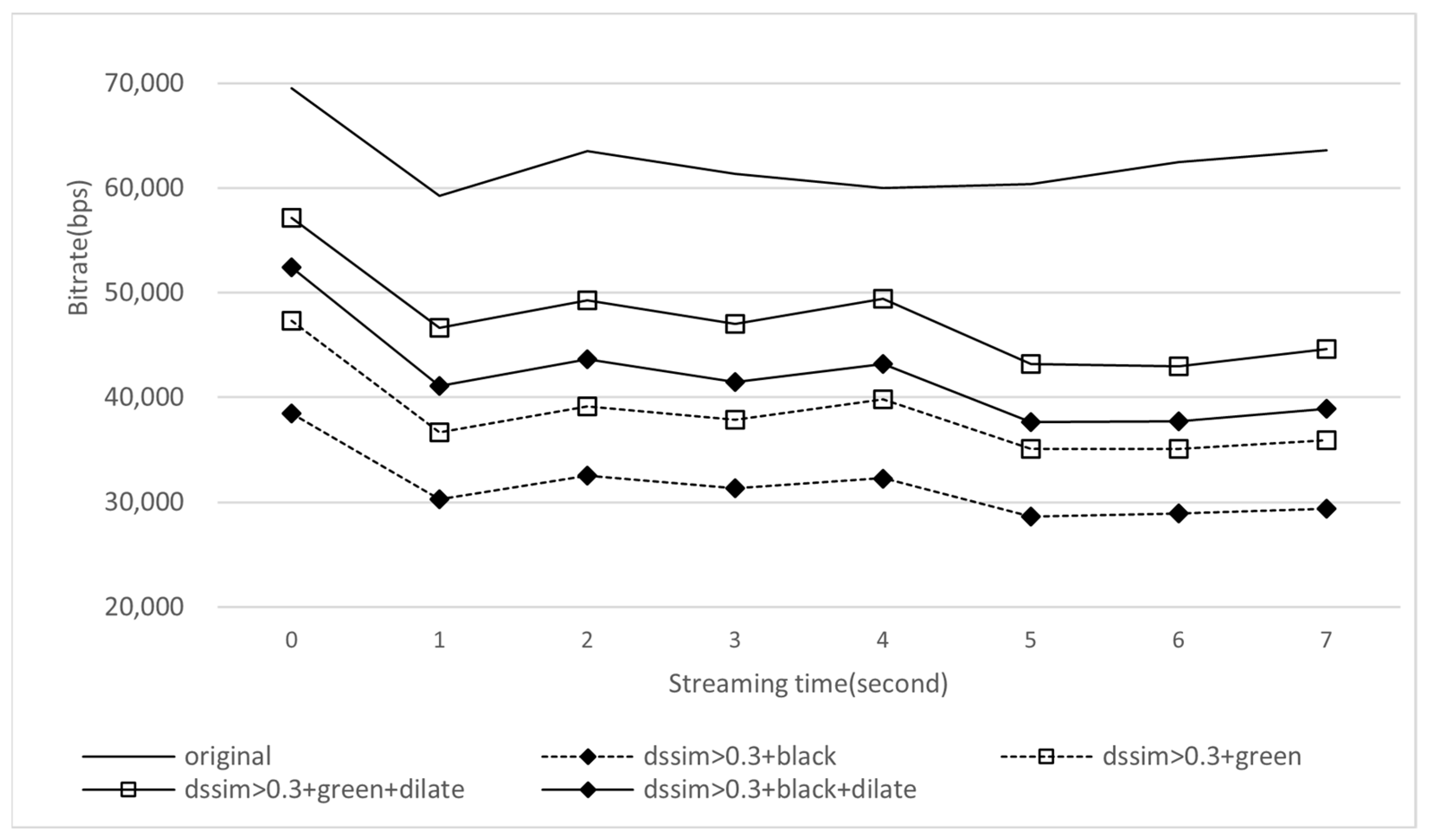
Based on the experimental results presented above, we could remain the areas of vehicles by properly removing the background without an overreaction to camera shake when the DSSIM threshold was set to 0.3. However, the performance of our model decreased because of damage to objectness caused by strong filtering with high DSSIM threshold values.

To deal with this problem, we applied two additional handlings for the input images of our model. First, we expanded the ROI areas in the DSSIM-MAP provided to the ROI filter. Because ROI areas are marked with black color in our study, their expansions can be done by image transformation with ‘dilate’ operations. We used a 3 × 3 size kernel for dilation and repeated this transformation five times. With this process, we can restore each object’s objectness damaged by ROI filtering. Figure 10 presents two images before and after performing the ROI expansions.

When comparing Figure 10a,b, the area in the foreground is expanded by dilation, reducing the amount of area of the object that is destroyed.

Second, we changed the color of non-ROI areas with a more saturated color so that they did not receive attention of a regional proposal network (RPN). This task was performed in the non-ROI color switcher. Since black, white, and red colors are generally used for the vehicle’s surface, headlights, and turn signals, an area with these colors can be misunderstood as a vehicle. Thus, we used the more saturated green color (RGB values: 0, 255, 0) for the non-ROI areas.

4.4.2. Bitrate

Figure 11 shows the bitrate change of video transmission when our two methods, ROI expansion and background coloring, were applied to enhance objectness of vehicles.

In Figure 11, the highest bitrate occurs when transmitting the original image, while the lowest bitrate was observed with the black background case without dilate operation applied. Additionally, we could confirm that applying dilate operation resulted in increased bitrates compared to cases without dilating.

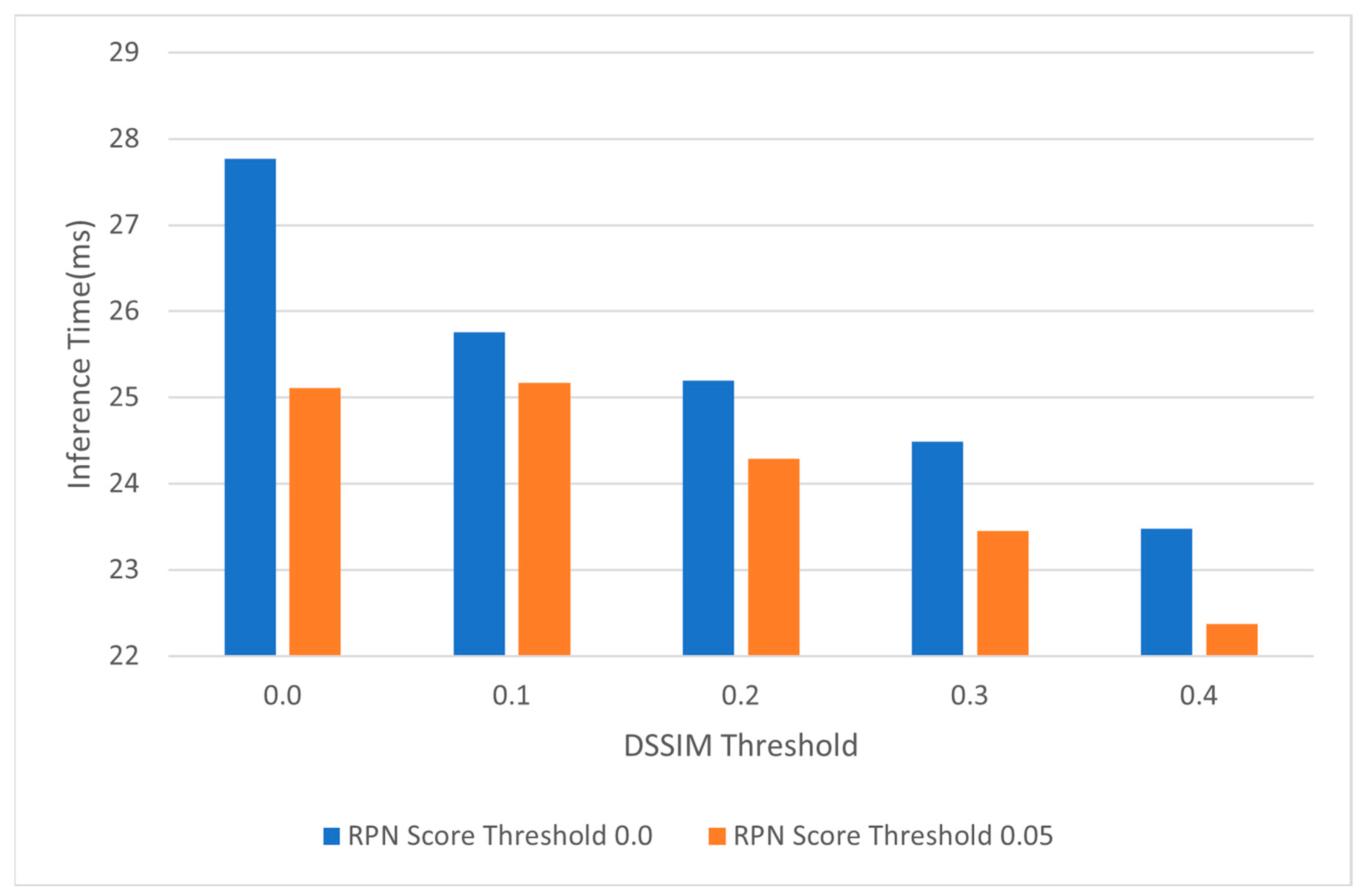
4.4.3. Inference Time

We measured the model’s inference times for videos by applying two methods to enhance the objectivities of vehicles described above. The length of each video is 240 frames, and the RPN score threshold of the model was configured with the default value of 0.05. Figure 12 illustrates the measurement results.

As shown in Figure 12, the model’s inference time slightly increased when the ROI expansion method was applied. For the colors of non-ROI areas, the inference time was shorter in the order of white, black, and green. Since shorter inference time implies that the areas proposed by the RPN had decreased, we can assure that the green color is more appropriate for our background coloring method to enhance the model’s performance.

4.4.4. Model Performance

To evaluate the performance enhancement achieved by our two methods for objectness enhanced images, we calculated again the model’s mAP and the precision, recall, and F1 score each object class.

Table 4. Inference Performance with different background colors and dilation application (DSSIM > 0.3).

Background Color and Dilation	Class	Precision	Recall	F1	mAP
white	Bus	0.62	0.81	0.70	50.65
	Car	0.51	0.65	0.57
	Truck	0.42	0.71	0.53
black	Bus	0.59	0.64	0.62	40.14
	Car	0.52	0.50	0.51
	Truck	0.50	0.48	0.49
green	Bus	0.64	0.83	0.72	66.20
	Car	0.59	0.91	0.72
	Truck	0.65	0.55	0.60
white with dilation	Bus	0.56	0.86	0.68	69.45
	Car	0.54	0.87	0.67
	Truck	0.43	0.89	0.58
black with dilation	Bus	0.57	0.85	0.68	70.98
	Car	0.54	0.87	0.67
	Truck	0.54	0.88	0.67
green with dilation	Bus	0.55	0.88	0.68	75.34
	Car	0.56	0.90	0.69
	Truck	0.59	0.90	0.71

presents the results.

The mAP was found to be around 40.14% in the black color background case. This is the same with that presented in Table 3 earlier. However, the mAP increased to be 50.65% and 66.20% when the background had filled with white and green colors, respectively. The F1 scores also increased in all the object classes when the background was colored with white or green.

When the ROI areas in the video were expanded with dilate operations, in all the cases of white, black, and green, the mAP considerably increased to be 69.45%, 70.98%, and 75.34%, respectively. Note that the mAP of YOLOv4 presented with the original dataset is around 68.2%, as described above.

5. Conclusions

This paper proposes an image-preprocessing method to reduce the data transmission and processing overhead for object detection in centralized IoT systems such as CCTV. The proposed method performs preprocessing to extract ROIs in the image with our DSSIM-based area filtering algorithm so that the object-detection model easily distinguishes objects from the background.

From experiments with our implementation, we could get some useful results. First, our image preprocessing method reduces ROI areas unnecessarily proposed by an RPN model so that the inference time for object detection is considerably reduced. Second, a video consisting of those preprocessed images requires less network resources to be transmitted to the server side. This can improve the utilization of centralized IoT systems including CCTV. Finally, the inference accuracy using those preprocessed images can be improved closely to the level of a case using original images if we sufficiently expand ROI areas in the image to enhance objectness and fill the background areas with a highly saturated single color such as green.

References

1. Navalgund, U.V.; Priyadharshini, K. Crime Intention Detection System Using Deep Learning. In Proceedings of the 2018 International Conference on Circuits and Systems in Digital Enterprise Technology (ICCSDET), Kottayam, India, 21–22 December 2018; pp. 1–6. [Google Scholar]
2. Liu, Y.-X.; Yang, Y.; Shi, A.; Jigang, P.; Haowei, L. Intelligent Monitoring of Indoor Surveillance Video Based on Deep Learning. In Proceedings of the 2019 21st International Conference on Advanced Communication Technology (ICACT), PyeongChang, Republic of Korea, 17–20 February 2019; pp. 648–653. [Google Scholar]
3. Girshick, R.; Donahue, J.; Darrell, T.; Malik, J. Rich Feature Hierarchies for Accurate Object Detection and Semantic Segmentation. In Proceedings of the 2014 IEEE Conference on Computer Vision and Pattern Recognition, Columbus, OH, USA, 23–28 June 2014; pp. 580–587. [Google Scholar]
4. Uijlings, J.R.R.; van de Sande, K.E.A.; Gevers, T.; Smeulders, A.W.M. Selective Search for Object Recognition. Int. J. Comput. Vis. 2013, 104, 154–171. [Google Scholar] [CrossRef]
5. Ren, S.; He, K.; Girshick, R.; Sun, J. Faster R-CNN: Towards Real-Time Object Detection with Region Proposal Networks. IEEE Trans. Pattern Anal. Mach. Intell. 2017, 39, 1137–1149. [Google Scholar] [CrossRef] [PubMed]
6. Girshick, R. Fast R-CNN. In Proceedings of the 2015 IEEE International Conference on Computer Vision (ICCV), Santiago, Chile, 7–13 February 2015; pp. 1440–1448. [Google Scholar]
7. Zhang, H.; Li, F.; Liu, S.; Zhang, L.; Su, H.; Zhu, J.; Ni, L.M.; Shum, H.-Y. DINO: DETR with Improved DeNoising Anchor Boxes for End-to-End Object Detection. arXiv 2022, arXiv:2203.03605. [Google Scholar] [CrossRef]
8. Carion, N.; Massa, F.; Synnaeve, G.; Usunier, N.; Kirillov, A.; Zagoruyko, S. End-to-End Object Detection with Transformers. arXiv 2020, arXiv:2005.12872. [Google Scholar] [CrossRef]
9. Redmon, J.; Divvala, S.; Girshick, R.; Farhadi, A. You Only Look Once: Unified, Real-Time Object Detection. arXiv 2016, arXiv:1506.02640. [Google Scholar] [CrossRef]
10. Du, B.; Du, H.; Liu, H.; Niyato, D.; Xin, P.; Yu, J.; Qi, M.; Tang, Y. YOLO-Based Semantic Communication With Generative AI-Aided Resource Allocation for Digital Twins Construction. IEEE Internet Things J. 2024, 11, 7664–7678. [Google Scholar] [CrossRef]
11. Zhu, X.; Su, W.; Lu, L.; Li, B.; Wang, X.; Dai, J. Deformable DETR: Deformable Transformers for End-to-End Object Detection. arXiv 2021, arXiv:2010.04159. [Google Scholar] [CrossRef]
12. Terven, J.; Cordova-Esparza, D. A Comprehensive Review of YOLO Architectures in Computer Vision: From YOLOv1 to YOLOv8 and YOLO-NAS. Mach. Learn. Knowl. Extr. 2023, 5, 1680–1716. [Google Scholar] [CrossRef]
13. Revathi, R.; Hemalatha, M. Moving and Immovable Object in Video Processing Using Intuitionistic Fuzzy Logic. In Proceedings of the 2013 Fourth International Conference on Computing, Communications and Networking Technologies (ICCCNT), Tiruchengode, India, 4–6 July 2013; pp. 1–6. [Google Scholar]
14. Song, Y.; Noh, S.; Yu, J.; Park, C.; Lee, B. Background Subtraction Based on Gaussian Mixture Models Using Color and Depth Information. In Proceedings of the 2014 International Conference on Control, Automation and Information Sciences (ICCAIS 2014), Gwangju, Republic of Korea, 2–5 February 2014; pp. 132–135. [Google Scholar]
15. Najar, F.; Bourouis, S.; Bouguila, N.; Belghith, S. A Comparison Between Different Gaussian-Based Mixture Models. In Proceedings of the 2017 IEEE/ACS 14th International Conference on Computer Systems and Applications (AICCSA), Hammamet, Tunisia, 30 October–3 November 2017; pp. 704–708. [Google Scholar]
16. Nurhadiyatna, A.; Jatmiko, W.; Hardjono, B.; Wibisono, A.; Sina, I.; Mursanto, P. Background Subtraction Using Gaussian Mixture Model Enhanced by Hole Filling Algorithm (GMMHF). In Proceedings of the 2013 IEEE International Conference on Systems, Man, and Cybernetics, Manchester, UK, 13–16 October 2013; pp. 4006–4011. [Google Scholar]
17. Yang, Y.; Liu, Y. An Improved Background and Foreground Modeling Using Kernel Density Estimation in Moving Object Detection. In Proceedings of the 2011 International Conference on Computer Science and Network Technology, Harbin, China, 24–26 February 2011; Volume 2, pp. 1050–1054. [Google Scholar]
18. Gidel, S.; Blanc, C.; Chateau, T.; Checchin, P.; Trassoudaine, L. Comparison between GMM and KDE Data Fusion Methods for Particle Filtering: Application to Pedestrian Detection from Laser and Video Measurements. In Proceedings of the 2010 13th International Conference on Information Fusion, Edinburgh, UK, 26–29 July 2010; pp. 1–7. [Google Scholar]
19. Akl, A.; Yaacoub, C. Image Analysis by Structural Dissimilarity Estimation. In Proceedings of the 2019 Ninth International Conference on Image Processing Theory, Tools and Applications (IPTA), Istanbul, Turkey, 6–9 November 2019; pp. 1–4. [Google Scholar]
20. Rouse, D.M.; Hemami, S.S. Understanding and Simplifying the Structural Similarity Metric. In Proceedings of the 2008 15th IEEE International Conference on Image Processing, San Diego, CA, USA, 12–15 October 2008; pp. 1188–1191. [Google Scholar]
21. Wang, Z.; Bovik, A.C.; Sheikh, H.R.; Simoncelli, E.P. Image Quality Assessment: From Error Visibility to Structural Similarity. IEEE Trans. Image Process. 2004, 13, 600–612. [Google Scholar] [CrossRef] [PubMed]
22. AI-Hub: CCTV Traffic Footage to Solve Traffic Problems (Highways). Available online: https://www.aihub.or.kr/aihubdata/data/view.do?currMenu=115&topMenu=100&aihubDataSe=data&dataSetSn=164 (accessed on 30 March 2025).
23. OpenCV: Background Subtraction. Available online: https://docs.opencv.org/3.4/de/df4/tutorial_js_bg_subtraction.html (accessed on 29 December 2024).
24. Bailly, R. Romigrou/Ssim 2024. Available online: http://github.com/romigrou/ssim (accessed on 29 December 2024).
25. Fasterrcnn_resnet50_fpn_v2—Torchvision Main Documentation. Available online: https://pytorch.org/vision/main/models/generated/torchvision.models.detection.fasterrcnn_resnet50_fpn_v2.html (accessed on 29 December 2024).
26. Loshchilov, I.; Hutter, F. Decoupled Weight Decay Regularization. arXiv 2019, arXiv:1711.05101. [Google Scholar] [CrossRef]
27. Padilla, R.; Netto, S.L.; da Silva, E.A.B. A Survey on Performance Metrics for Object-Detection Algorithms. In Proceedings of the 2020 International Conference on Systems, Signals and Image Processing (IWSSIP), Niterói, Brazil, 1–3 July 2020; pp. 237–242. [Google Scholar]
28. JeonHyeonggi JeonsLab/Roi_extract_data 2025. Available online: https://github.com/jeonslab/roi_extract_data (accessed on 30 April 2025).
Figure 1. Architecture of Faster R-CNN.
Applsci 15 05328 g001
Figure 2. Overview of proposed method.
Applsci 15 05328 g002
Figure 3. Visualization examples of a portion of the dataset: The dataset consists of images and annotations, with classes and bounding boxes labeled for vehicles. In this image, magenta color boxes represent truck labeling, while green color boxes represent car labeling.
Applsci 15 05328 g003
Figure 4. Result of the reference image generator operation: moving objects are removed, presenting only the background.
Applsci 15 05328 g004
Figure 5. Operation result of the DSSIM Generator: brighter areas indicate regions that differ from the background.
Applsci 15 05328 g005
Figure 6. Filtering results with different DSSIM threshold values.
Applsci 15 05328 g006
Figure 7. Bitrate on video transmission with different DSSIM threshold values.
Applsci 15 05328 g007
Figure 8. Training—validation loss curves during training model.
Applsci 15 05328 g008
Figure 9. Inference speed based on RPN score thresholds and DSSIM thresholds.
Applsci 15 05328 g009
Figure 10. Two images before and after ROI expansions: (a) example of DSSIM filtered image which was damaged in objectness; (b) processed image with dilate method for restoring objectness.
Applsci 15 05328 g010
Figure 11. Bitrate on video transmission with ROI expansion and background coloring. Because both bitrates of the white and black background cases appeared very similar, we presented result of only black cases in the figure.
Applsci 15 05328 g011
Figure 12. Inference time with difference operations: Three colors were applied to the non-ROI areas, and the dilate operation was either applied or not applied.
Applsci 15 05328 g012