Enhancing Asset Reliability and Sustainability: A Comparative Study of Neural Networks and ARIMAX in Predictive Maintenance

Abstract

Organizations strive to maximize efficiency in their manufacturing processes, yet they must also consider broader repercussions, as industrial activity directly impacts the environment and society. The adoption of innovative technologies and initiatives to mitigate this impact is therefore essential. Traditional asset maintenance plays a critical role in ensuring high equipment availability, but there is a clear need to evolve toward predictive and sustainable maintenance strategies to enhance reliability, safety, and equipment lifespan. This shift redefines maintenance itself, aligning it with circular economy principles and Industry 4.0 solutions to prevent unplanned downtime, reduce failures, and improve personnel and facility safety. This research examines the transition from traditional preventive maintenance to predictive and sustainable maintenance in a real-world industrial context, comparing the design of a neural network with the ARIMAX technique to develop reliable predictive models. The study aims to facilitate a paradigm shift by proposing a predictive model that reduces unplanned shutdowns and optimizes spare parts and labor utilization. The practical application focuses on a hydrogen compressor in the petrochemical industry, demonstrating the model’s potential for operational and sustainability improvements.

1. Introduction

The renewed impetus for the 2030 Agenda [1], combined with the emergence of Industry 4.0, aimed to modernize manufacturing via sustainable processes, cyber-physical systems, the Internet of Things (IoT), and cloud computing [2]. These developments are particularly relevant to asset maintenance, which traditionally falls into three categories: (1) corrective maintenance: reactive repairs after unexpected failures; (2) preventive maintenance: scheduled component replacements based on time or usage intervals, and (3) condition-based maintenance: real-time monitoring using sensors to predict failures without physical inspection [3].

The rise in Industry 4.0 technologies (e.g., IoT, big data analytics) has revolutionized condition-based approaches by enabling continuous data collection, fault prognosis, and dynamic maintenance planning. This shift enhances productivity, sustainability, and asset lifespan estimation while reducing unplanned downtime. This predictive approach is only applicable to monitored equipment, as it relies on sensor-derived data to accurately estimate asset lifespan [4]. By integrating real-time data, maintenance strategies—including condition monitoring, fault diagnosis, prognosis, and planning—are dynamically optimized [5]. The evolution of manufacturing paradigms, from mass production to lean manufacturing, reflects growing societal demands for greener and more sustainable industrial practices. Modern companies must balance economic growth with social and environmental responsibility [6]. Sustainable manufacturing embodies this shift, emphasizing resource efficiency, cleaner technologies, and safeguards for both environmental integrity and human health [7,8]. To achieve these goals, a transition from a linear to a circular economy is essential. This systemic change prioritizes waste reduction through policies promoting recycling, reuse, remanufacturing, and material recovery—all while maintaining economic viability [9,10,11].

The EN 16646 standard [12] emphasizes that effective maintenance policies must integrate diverse perspectives by understanding the interdependencies between operations and value creation across the asset lifecycle. The transition from preventive to predictive and sustainable maintenance can be framed within the continuous improvement paradigm. Continuous improvement traces its origins to the mid-20th century with W. Edwards Deming’s development of the PDCA (Plan–Do–Check–Act) cycle [13], a four-stage iterative problem-solving framework. This methodology can be systematically applied through the following stages: diagnosis (problem description and analysis), root cause analysis, definition of countermeasures and target values, implementation, monitoring, and standardization [14]. Therefore, the “Plan” phase comprises: (1) redefinition of key performance indicators (KPIs) and target asset selection, (2) sensor selection and deployment, and (3) data collection, analysis, and storage. The “Do” phase involves: (4) predictive model development, and (5) staff training and competency development. The “Check” phase includes: (6) solution validation and performance monitoring within a defined temporal scope. Finally, the “Act” phase involves: (7) scaling the implementation to additional assets, the standardization of procedures, and monitoring to prevent performance degradation over time (as illustrated in Figure 1). Once the “Act” phase is completed, a decision is made either to replicate the solution in new facilities and/or assets or—if the results have not met expectations—to restart the cycle to achieve the objectives initially planned. For comprehensive guidance on implementation tools, methodologies, and critical success factors, refer to [15,16,17,18,19].

1.1. Considerations in the Preparation of the Predictive Maintenance Plan

This paper focuses on predicting the operational behavior of a hydrogen compressor in a petrochemical facility producing caprolactam, a precursor for nylon 6 fibers. Given the continuous nature of the manufacturing process, any component failure can lead to full production stoppages. Unplanned shutdowns entail significant risks, including collateral damage to critical components (e.g., sensors, control valves, pipelines, and electrical systems), delayed customer deliveries, and increased costs for emergency spare parts and overtime labor.

Although the compressor has experienced few failures in recent years, emerging electromechanical issues—such as bearing wear due to overheating and power supply instability—highlight the need for proactive solutions. Additionally, missing data values in other equipment records, attributed to aging communication infrastructure and lack of signal redundancy, further complicate predictive efforts. These challenges have been formally assessed by multidisciplinary teams, confirming the urgency of addressing both hardware and data reliability gaps. Implementing these enhancements in the hydrogen compression process is expected to yield the following benefits:

• Reduction in Unplanned Downtime: Minimizing emergency stops caused by malfunctions or missing data values, thereby avoiding subsequent inspections, refurbishments, or replacements of damaged components.
• Improved Decision-Making for Operators: Providing reliable, data-driven insights to operators enables controlled shutdowns when necessary. In optimal scenarios, this allows continued operation until scheduled maintenance can address the issue.
• Enhanced Sensor Infrastructure: Rewiring sensors to ensure signal redundancy may require new hardware and software modifications to process duplicated data streams effectively.
• Increased System Reliability: Evaluating the acquisition of a twin compressor could further enhance reliability through redundancy, ensuring uninterrupted operation.

Sustainable maintenance management represents a critical strategy for achieving sustainable development [20], requiring organizational shifts in policies, strategies, and asset maintenance practices [21,22]. This approach expands the traditional triple-bottom-line framework of sustainable maintenance [23] by incorporating a fourth, technology-driven dimension [24]. The resulting four dimensions are defined as follows:

• Economic Dimension: Focused on operational efficiency, downtime reduction, process quality, and overall productivity [25,26].
• Environmental Dimension: Centered on resource optimization and waste minimization [27,28,29,30].
• Social Dimension: Encompassing legal compliance regarding employee health/safety and customer obligations [31].
• Technological Dimension: Addressing the integration of advanced technologies into maintenance systems [32,33,34,35].

The transition to sustainable maintenance necessitates adopting new performance metrics. Notably, the EN 15341 standard [36] outlines 183 maintenance management indicators, including, 3 directly tied to sustainability, 22 related to health, safety, and environment (HSE), 21 concerning personnel competence, and 20 focused on Industry 4.0 technologies. A comprehensive maintenance plan should integrate at least one indicator from each sub-function to enable holistic performance assessment. The adoption of condition-based maintenance is significantly enhanced by Industry 4.0 technologies, which are fundamentally characterized by cyber-physical systems (CPS). These CPSs are characterized by a tight integration of physical and computational systems, enabling actuators deployed in the real world to operate adaptively and autonomously based on signals from sensor inputs [37].

Deep belief networks (DBN), introduced by [38], is a type of neural network widely employed in predictive maintenance tasks due to their hierarchical learning capability, which enables capturing long-range dependencies—primarily in unsupervised learning. This architecture can be used in both supervised and unsupervised frameworks, being mainly applied for data dimensionality reduction and classification [39,40]. However, DBNs are not suitable for time series prediction, as they have been outperformed by deeper architectures such as LSTMs and Transformers [41,42].

Unlike traditional statistical forecasting methods such as autoregressive moving average (ARMA) [43], autoregressive integrated moving average (ARIMA) [44], autoregressive integrated moving average with exogenous variables (ARIMAX) [45], and exponential smoothing [46], which are typically limited as they rely on a sole time series, neural networks provide a promising solution for handling massive data [47], and they are characterized by multiple layers that enable complex feature abstraction from data points [48].

For the purpose of anticipating possible problems, Kanawaday and Sane [49] indicates that smart maintenance within Industry 4.0 is oriented towards self-learning, failure prediction, diagnosis, and triggering maintenance programs. At the same time, Zeng et al. [50] identifies the suitability of its application since the utilization of supervised models for making forecasts will ensure that the process operates correctly and efficiently without incurring high maintenance costs and reducing product or assets degradation. Machine learning refers to the set of techniques and methods used by computers to autonomously extract complex patterns and relationships from large datasets and make decisions or predictions about real-world events [51]. The concepts used in machine learning are cross-disciplinary and come from computer science, statistics, mathematics, and engineering. The main types of machine learning were outlined by [52], and predictions are made based on new or unanticipated data [53] using labeled dataset. Deep learning is a branch of machine learning that focuses on the learning of data representations and of hierarchical features. With the objective of extracting features, deep learning algorithms employ a system comprising numerous layers of nonlinear processing identities (neurons) that aid in data abstraction [54]. Although recurrent neural networks in their various forms have traditionally been used, architectures equipped with attention mechanisms commonly used in natural language processing, which are more complex and have a higher number of trainable parameters, should provide better results [55]. The full discussion of Transformer-based neural networks for time series prediction can be found in [56].

For a comprehensive analysis of machine learning strategies and their application to predictive maintenance in sustainable manufacturing, readers may consult references [57,58]. The optimization of neural network hyperparameters is conducted through Design of Experiments (DoE) methodology, with the dual objective of maximizing model performance, while ensuring operational simplicity to facilitate adoption by practitioners with limited technical expertise in machine learning.

The implementation of this combination of solutions requires careful consideration and resolution of several difficulties, including the choice of technology to invest in, the management of current knowledge, its transfer, and the acquisition of new expertise [59,60] describes the implementation of a roadmap that optimizes the likelihood that these tools will be applied successfully. These improvements are benchmarked against traditional forecasting methods like ARIMAX, a generalized ARIMA framework that integrates exogenous variables to improve predictive capability.

The evaluation and integration of these new requirements are designed to enhance the likelihood of successfully implementing an intelligent and sustainable maintenance system, as opposed to relying solely on a traditional preventive maintenance approach.

1.2. Contribution of the Paper

In summary, this study aims to optimize resource utilization (technical, economic, and human) through systematic parameterization of a Transformer-based neural network, with three key objectives:

Signal Reliability Assessment:

To evaluate whether statistical and technical tools can effectively determine if secondary variables provide reliable predictive information about process behavior, thereby creating signal redundancy.

Computational Efficiency Optimization:

To optimize neural network hyperparameters for maximum computational efficiency, minimizing training/retraining resource requirements, while benchmarking performance against simpler methodologies.

Practical Implementation Evaluation:

To assess the suitability of this forecasting tool for integration into maintenance plans, considering operational complexity and computational demands relative to alternative, simpler approaches.

1.3. Structure of the Document

The structure of this paper is organized as follows: Section 1 presents a comprehensive overview of Industry 4.0’s foundations, sustainable manufacturing principles, and maintenance function evolution, highlighting their practical applications to real-world industrial challenges. Section 2 describes the facility’s operational characteristics and details the data acquisition methodology from the target equipment. Section 3 provides a technical exposition of the Transformer-based neural network architecture employed in this study. Section 4 presents the statistical optimization framework, including the Design of Experiments methodology. Section 5 and Section 6 analyze and discuss the obtained statistical results. Section 7 examines both the technical challenges confronting these solutions and the organizational barriers to their implementation. Finally, Section 8 synthesizes the key findings, draws substantive conclusions, and proposes actionable directions for future research.

2. Description of the Equipment, Facilities, and Data Collection

A multistage (4-stages) hydrogen compressor is used to compress the gas from 0.034 MPa to 27.95 MPa, cooling the hydrogen after each stage to prevent its temperature from reaching above 423 K. According to [61], the present level of preventive maintenance corresponds to level 3, as there exists a monitoring and alarm system that alerts operators in the event of any anomalies, in addition to the mandatory preventive maintenance every three months.

The objective is to implement Industry 4.0 technologies with the aim of enhancing maintenance up to level 4 and reducing the over maintenance through the utilization of real-time data monitoring based on predictive techniques. The acquisition of knowledge involves the training of a neural network that employs self-attention mechanisms to identify the hyperparameter configuration that most effectively aligns with the type of data generated by sensors. Due to the enormous volume of real-time sensor data generated in facility operations, a highly specialized distribution control system is implemented in order to enable efficient analysis and decision-making. Figure 2 illustrates how data are collected through the asset’s sensors and connected via Ethernet to the control racks, which then send the signal to the unique database, which then shares the data through the OPC-UA server for subsequent processing by users. No data can be managed or stored either on the cloud or external servers due to the organization’s current security policy, thus the raw sensor data are transmitted directly to clients, who process the monitoring in real-time through a SCADA system and adjust variable values as required to prevent out-of-range operating situations.

Two separate wirings comprise the sensors: one monitors endogenous variables, while the other monitors exogenous ones. The variables are grouped based on the connection in

Table 1. Grouping sensors by wiring connection and nominal values of each variable.

Exogenous Variables	Endogenous Variables
Fresh H2 flow (500 Nm3/h) Cooling flow (Nm3/h), undefined	H2 outlet pressure; Stages 1–4 (0.39/1.97/8.29/28.4 MPa)
H2 inlet temperature (318 K)	H2 temperature; Stages 1–4 (418/398/403/403 K)
	Compression ratio; Stages 1–4. (11.5/5.0/4.2/3.5 Dimensionless)
	H2 post intercooling pressure (27.95 MPa)
	H2 post intercooling temperature (373 K)
	rpm (min−1); undefined Compressor consumption (300 A)

. The variable to be predicted is “H₂ post intercooling pressure” or simply outlet pressure.

The hydrogen pressure is performed by an absolute pressure stainless steel transmitter designed for explosion environments. This device features a piezoresistive metallic diaphragm and can operates over 30 MPa with a PROFIBUS—PA compatible analog output (4–20 mA). The current measurement device is a three-phase connection and 0–400 A measurement range with PROFIBUS-PA compatibility.

The equipment produces data points every minute, with the output pressure nominally set at 27.95 MPa and controlled within limits of 25.99 and 29.91 MPa. With the objective of stabilizing the process and improving the predicting capacities of the neural network, it is necessary for operation to occur on a fifteen-minute basis and it is imperative to adjust the control limits to align with the new average values. This makes it easier to predict the next few hours of operation, as opposed to predicting the equipment’s behavior over the next few minutes. By applying the central limit theorem, the new limits for the average out pressure have been established at 27.44 and 28.45 MPa utilizing the expression σ = (29.91 − 25.99)/(6√15) to estimate the new standard deviation. Thus, the new limits control will be set at ±3 σ.

Controlled and emergency stops are the two types of stoppages that an operator can perform. The latter is carried out in a shorter time and can cause the greater degradation of the compressor components. In addition, the training processes for control operators are extensive due to the absence of any technological support for decision-making. Every action requires collaboration with highly experienced operators until trainees attain the necessary expertise and confidence to accurately assess the situation, thereby minimizing the risk of a full system shutdown.

The data presented in Figure 3 reflect fifteen-minute averages of both the outlet hydrogen pressure and the main motor’s current consumption. As illustrated, five scheduled equipment shutdowns—associated with preventive maintenance—are evident, with the most prolonged interruption occurring during the summer months.

The maintenance team focuses on inspecting and replacing components according to established work protocols and standards. If the increased deterioration of any component is observed during a planned maintenance intervention, adjacent components that may be affected are also inspected and repaired. However, there are currently no dedicated teams that systematically investigate the root causes of these issues following a defined methodology.

3. Self-Attention Neural Network

The network known as Transformer, originally designed for natural language processing, uses only attention mechanisms to predict the output sequence instead of long short-term memory (LSTM) networks along with attention mechanisms of type [62,63] as were previously implemented in these types of solutions. The innovative approach of Transformers involves three distinct attention architectures: self-attention for input data in the encoder, masked attention for the predicted sequences in the decoder, and finally, cross-attention, wherein the information from the encoders and the decoders, specifically from masked attention, are combined.

The model inspired by [42] captures dependencies between distinct points in the time sequence, although instead of employing all parts of the Transformer network, including encoders and decoders, to predict the behavior of time series values, only the self-attention mechanism of the encoder is used along a feed-forward layer to obtain the output tensor.

Therefore, Figure 4 shows the network used, in which the normalized sequence of data to be predicted is introduced into a normalization layer before it enters multi-head attention block. Batch normalization is a regularization technique that is applied to input layers consisting of normalizing the activation values of the units in that layer so that there is a mean of 0 and a standard deviation of 1 [64]. This improves stability and facilitates the convergence speed while avoiding problems such as exploding or vanishing gradients. You should not confuse batch normalization with input data normalization, which involves scaling input data to a specific range to improve numerical representation.

The attention block uses three independent networks: query (Q), key (K), and value (V) to acquire information from the input data and obtain a proper representation of it. The block calculates the attention weight by dividing the dot product between the query and key vectors by a scaling factor (d), transforming it using the SoftMax function to obtain numerical values between 0 and 1, and finally multiplying it by the value vector (Equation (1)) to condense the information into a vector for each data point or token.

This set of layers and blocks forms the normalization and multi-head attention block. Multiple attention blocks can be used to detect further associations and relationships among data points and/or groups of data across different levels. These vectors are then combined using an additional neural network into a single compressed vector. Furthermore, a dropout layer is applied to its output [65] in order to prevent the excessive overfitting of the model.

$$Attention\left(Q,K,V\right)=softmax\left({\displaystyle \frac{Q{K}^T}{\sqrt{d_k}}}\right)V$$

(1)

The obtained vector is then added to the normalized input sequence and introduced into the feedforward layers, which consist of a normalization layer, a dropout layer, and two 1D convolutional layers. Finally, the output is added to the input of this layer, forming the encoder structure. Due to their feature extraction capability, convolutional networks are commonly used in data from numerical series.

Convolutional networks are a type of dense, feed-forward neural networks that have been successfully applied in many domains [66], such as classification problems or time series classification [67]. This structure of the model enables the recognition of specific patterns and the abstraction of information from the input sequence. This architecture is called an encoder, and it can be repeated up to six times in succession. A global average polling 1D layer (GAP1D) is added to the output of the encoders for polling, preserving all relevant information in a single layer that is easily understood by dense layers equipped with another dropout layer to obtain the time series forecast.

Once the self-attention mechanism network architecture has been defined, it is necessary to empirically analyze it and determine the value of hyperparameters that maximize the result (lower MAE or RMSE) with the lowest computational cost. Statistical analysis allows only considering relevant factors, which result in a simpler model to train.

Python (v. 3.11.12) and specifically its Keras (v. 3.8.0) and Tensorflow (v. 2.18.0) libraries have been used to design the neural network, which are intended for the creation of deep learning models and networks. They also allow great flexibility by allowing user-customizable configurations.

4. The Concepts and Procedures for the Utilization of Design of Experiments (DoE), ARIMAX, and Bootstrap

Most practical situations where it is intended to control the output or response of a real process are conditioned by the existence of controllable variables (factors) and other unknown factors. The DoE is a methodology proposed by Ronald A. Fisher [68] and it encompasses a set of mathematical and statistical techniques that seek the effects on a measured response variable (Y) by simultaneously manipulating certain input variables (Xs).

In the application of DoE techniques, the main guidelines may include the following: (1) stating the objectives of the research, (2) defining the response variable(s), (3) determining factors and levels, (4) deciding the experimental design type, (5) conducting the experiment, (6) data analysis, and (7) validation of the results. With the intention of estimating first and second order effects and cross-product, two-level factorial designs are used, and the polynomial function must contain quadratic terms. An orthogonal design is shown in the equation below:

$$y={\beta }_0+{\sum }_{i=1}^k{\beta }_i{x}_i+{\sum }_{i=1}^k{\beta }_{ii}{x}_i^2+{\sum }_{1\le i<j}^k{\beta }_{ij}{x}_i{x}_j+\epsilon$$

(2)

where $k$ is the number of variables, ${\beta }_0$ is the constant term, ${\beta }_{\mathrm{i}}$ represents the coefficients of the linear parameters, $x_i$ represents the variables, ${\beta }_{\mathrm{i}\mathrm{i}}$ represents the coefficients of the quadratic parameters, ${\beta }_{\mathrm{i}\mathrm{j}}$ represents the cross-product, and $\epsilon$ is the residual associated with the experiment (random error).

The variables are usually expressed in different units and vary in different ranges, which makes it necessary to code them. If this is not accomplished, it is impossible to assess the relevance of a factor through the magnitude of the model coefficients. As a result, all factor levels are set at two levels (−1, +1) with equal spaced intervals between them.

Hence, the factorial experiments with multiple factors with two levels (“high” and “low”), suggest that the complexity of the model grows exponentially (2^k), and the experiment requires a lot of resources and time. Since a low number of main effects and lower order interactions are significant to the response variable, and higher order interactions are not significant, a fractional factorial design may be chosen.

As an extension of the widely used ARIMA (autoregressive integrated moving average) forecasting model, the ARIMAX allows for the inclusion of one or more exogenous variables, thereby enabling more satisfactory predictions. The model can be expressed as follows:

$$\left(1-{\varphi }_{1}L-\dots -{\varphi }_p{L}^p\right){\left(1-L\right)}^d{y}_t=c+\beta X_t+{(1+\theta }_{1}L+\dots +{\theta }_q{L}^q){ϵ}_t$$

(3)

where $y_t$ is the value of the time series at time t, $X_t$ is the exogenous variable at time t, $\beta$ is the coefficient that measures the impact of the exogenous variable, ${\varphi }_1,\dots ,{\varphi }_p$ are autoregressive coefficients, ${\theta }_1,\dots ,{\theta }_q$ are moving average coefficients, c is de average level of the time series when all other variables are zero (AR(p), MA(q), $\beta$), L in the lag operator, and finally, ${ϵ}_t$ is the error term at time t. The proper use of this model requires the time series to be stationary, i.e., it must have constant mean and variance over time. To verify this condition, the Dickey–Fuller (ADF) test is employed, where the null hypothesis (H₀) states that the series is non-stationary, against the alternative hypothesis (H₁) that the series is stationary. If the series is found to be non-stationary, it must be differentiated until stationarity is achieved. The determination of the AR and MA orders is guided by the ACF and PACF plots. Additionally, if the ACF exhibits a slow, gradual decay, this is a clear indicator of non-stationarity in the series.

Similarly, in cases where it is desired to estimate the parameters of an unknown data distribution, it is common to use the Bootstrap technique, introduced by Efron in 1979 [69]. This method involves creating new datasets from an existing sample by employing resampling with replacement. The Bootstrap principle starts with a random sample from an unknown distribution $X=\left\{x_1,x_2,\dots ,x_n\right\}$, and B resamples $X_1^{\ast },X_2^{\ast },\dots X_B^{\ast }$, each of size n, are generated. For each resample $X_b^{\ast }$, the statistic of interest is computed ${\widehat{\theta }}_b^{\ast }$, and the empirical distribution of ${\widehat{\theta }}^{\ast }\left(X\right)$ is used to approximate the sampling distribution of the statistic. There is extensive literature on this topic, so I encourage interested readers to consult [70]. The desired estimator is then computed on the datasets generated, and this estimator will approximate the (unknown) estimator evaluated on the actual population.

5. Use of Artificial Neural Network

This methodology relies on historical data, where hyperparameter values are adjusted simultaneously to identify those most influential on the network’s performance, aiming to minimize specific outputs. These outputs include the mean absolute error (MAE) defined in Equation (4), computing time per epoch, and the number of trainable parameters.

$$MAE=\sum _{t=1}^T{\displaystyle \frac{|{\widehat{y}}_t-y_t|}{T}}$$

(4)

Here, $y_{t }$ represents the true output, ${\widehat{y}}_t$ denotes the estimated output T corresponds to the number of data points. To manage computational complexity and resource efficiency, a reduction strategy is often necessary to limit the number of experimental runs, as the complexity scales with the number of hyperparameters.

Table 2. Hyperparameters considered in the model.

	Hyperparameter	−1	1		Hyperparameter	−1	1
A	Sequence size	5	35	E	No. encoder blocks	2	6
B	Head size	64	192	F	mlp units	64	192
C	Number of heads	2	6	G	Learning rate	0.0005	0.0015
D	F. Forward dimension	2	6

outlines the factors evaluated in this study to determine the optimal network size for minimizing prediction errors on the provided dataset. It is important to note that these factors are presented as normalized and encoded values, ranging from −1 to 1.

The sequence size (A) denotes the number of data points extracted from the temporal sequence that are utilized for network training to generate the forecast. The head size (B) corresponds to the number of neurons comprising each attention head. The number of heads (C) represents the quantity of independent attention mechanisms embedded within the Transformer block. The feedforward dimension (D) specifies the count of one-dimensional convolutional layers. The number of encoder blocks (E) indicates the total number of encoder layers that constitute the network. The MLP units (multi-layer perceptron units—F) define the number of neurons within the fully connected dense network, while the learning rate (G) determines the magnitude of the adjustment step taken during each iteration to minimize the loss function.

To minimize the computational demands on the hardware, relevant hyperparameters are optimized to their ideal values, while non-essential factors are set to their minimum thresholds. The neural network is subsequently trained using historical data, concurrently with the collection of new data from the compressor. The model generates predictions in the form of a time series. Based on the model’s training, the predicted data, and their operational expertise, control room technicians evaluate the potential implications of equipment operating outside acceptable ranges or experiencing unplanned shutdowns. Decisions are then made in accordance with established operational protocols.

Given the considerable number of factors under consideration (7), the adoption of a fractional factorial design is considered necessary. The resolution of the design is determined by the number of experimental runs required and the acceptable degree of aliasing among the factors, including their second-order, third-order, and higher-order interactions. Consequently, a resolution IV design is selected as the minimal configuration capable of capturing the most significant main effects and second-order interactions. While this design results in aliasing between factors and second-order interactions, it is deemed the most suitable option based on the established assumptions. By employing this design, only 16 experimental trials are required, as opposed to the 128 trials needed for a full factorial design, and two replications are included.

Figure 5 illustrates the process followed. The data have been divided into three subsets: training (70%), validation (15%), and testing (15%). The hyperparameters are adjusted according to the determinations made in the DoE, and the MAE values for the validation data are calculated. Once the model with the optimum MAE is identified, the residuals are determined to establish the prediction limits. The testing data are used to assess whether the network possesses the desired predictive capability.

The columns of

Table 3. MAE. Results of the experiment for validation and test data.

No.	Run 1		Run 2		Run 3		s/Epoch (Average)	Trainable Param.
	Val.	Test	Val.	Test	Val.	Test
1	0.1452	0.1930	0.1291	0.1746	0.1224	0.1688	3.243	14,513
2	0.0833	0.1297	0.1161	0.1429	0.0814	0.1247	2.455	17,609
3	0.1049	0.1371	0.0989	0.1328	0.1045	0.1311	2.735	20,497
4	0.1483	0.1992	0.1693	0.2115	0.1509	0.2029	17.391	57,545
5	0.1344	0.1919	0.1143	0.1798	0.1252	0.1852	3.017	32,665
6	0.1304	0.1561	0.0903	0.1308	0.1034	0.1330	2.799	17,681
7	0.1225	0.1418	0.1174	0.1396	0.1230	0.1505	1.310	6,065
8	0.1111	0.1473	0.1186	0.1519	0.1118	0.1528	1.355	3,225
9	0.1154	0.1564	0.1174	0.1585	0.1313	0.1646	1.460	17,585
10	0.0899	0.1619	0.0892	0.1653	0.0528	0.1448	3.500	32,713
11	0.1024	0.1672	0.1009	0.1651	0.0532	0.1467	17.294	75,793
12	0.1041	0.1384	0.0925	0.1245	0.1092	0.1370	2.835	20,425
13	0.1182	0.1760	0.1225	0.1821	0.1632	0.2055	2.333	32,689
14	0.1579	0.1904	0.1018	0.1667	0.1600	0.1962	2.060	14,489
15	0.1177	0.1388	0.1039	0.1255	0.1173	0.1532	1.775	20,377
16	0.1595	0.2081	0.1192	0.1745	0.1176	0.1724	3.435	14,609

display the MAE obtained for the validation and testing data for each configuration of the neural network and its replicates. Additionally, the average computation time per epoch in seconds is included, along with the number of trainable parameters, which provides an indication of the network’s complexity.

From the response surface model for the MAE of the validation and testing data, it is inferred that the significant factors are the size of the data series (A), the number of encoder blocks (E), the size of the multilayer perceptron (F), and the learning rate (G). Additionally, the normality of the data allows for the application of ANOVA, leading to the conclusion that the mean errors of the two data groups (validation and testing) are significantly different, which may be attributed to various underlying causes. The presence of data drift or data shift refers to a change in the distribution of the predictors, a change in the distribution of the target variable, or a change in the relationship between the predictors and the target variable. This phenomenon leads to a progressive decline in the model’s predictive accuracy [71]. An additional factor contributing to this issue is the model’s tendency to overfit the validation and training data, which compromises its ability to generalize effectively to new testing datasets. Resolving this challenge is non-trivial, and [72] highlights that the root causes often lie in the use of excessively complex models with a high number of trainable parameters or the model’s inadvertent assimilation of noise inherent in the data series.

To further analyze the network, a design is implemented in which the discarded variables (B, C, and D) are fixed at their maximum, median, and minimum values, verifying whether the variables excluded by the DoE truly have no impact on the network’s performance. Figure 6 presents the boxplot of the validation and test values, highlighting the non-significant factors and enabling the clear observation of distinct processes.

After analyzing the normality of the obtained MAE values, ANOVA is performed on the normally distributed data, and the non-parametric Kruskal−Wallis test is applied to the non-normal distributions (test data). In both cases, it is concluded that the most complex architecture yields the lowest MAE, although the input data series must be the shortest. Likely, the use of a larger number of data points in the input series introduces additional noise into the network, resulting in poorer predictions. Therefore, the optimal architecture corresponds to the network (A = 20, B = 192, C = 6, D = 6, E = 2, F = 64, G = 15; MAE_Val = 0.06289 and MAE_Test = 0.09573).

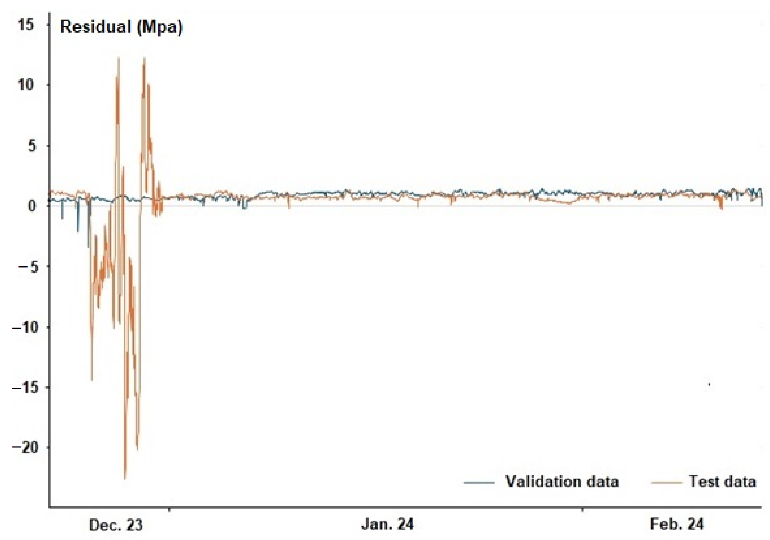
Figure 7 illustrates the residuals of the validation and test data, which represent the difference between the observed actual values and those estimated by the neural network. It is readily apparent that the residuals exhibit bias, specifically 0.91 MPa, indicating that the predicted values are systematically lower than the actual values. Furthermore, the distributions of these residuals are non-normal.

The erratic behavior of the test data residuals stems from the fact that the original series includes a planned preventive maintenance shutdown, which is where the neural network exhibits the greatest difficulty in making accurate predictions. Beyond this event, both series demonstrate similar behavior.

Additionally,

Table 4. Characteristics of the residuals.

		Val. Data	Test Data	Test Data *
Residuals $(y_t-{\widehat{y}}_t)$	Bias	0.9165	0.3561	0.7906
	Standard deviation	0.2826	2.6777	0.2039
	Normally distributed	No	No	No

* The first 1000 data points of the series are excluded (maintenance time).

presents the characteristics of the residuals for both series, as well as the residuals corresponding to the test data, excluding those associated with the year-end preventive maintenance shutdown.

To evaluate the relationship between the actual and predicted data, the degree of correlation between the original data and their predictions can be measured. For this purpose, the Pearson and Spearman correlation coefficients, as well as Kendall’s tau [73], can be employed. These coefficients measure the relationship between two variables in different ways. Refer to

Table 5. Correlation coefficients between the actual and estimated data.

Data	Pearson	Spearman	Kendall Tau
Validation	−0.3160	−0.4022	−0.2732
Test	0.9243	0.5135	0.3695

.

While the correlation between the actual and predicted data in the validation group exhibits an inverse relationship—that is, there is a tendency for one variable to decrease as the other increases—the test data, in contrast, shows a direct correlation. From this divergent behavior, it can be inferred that the compression process captured in the test and validation data differs.

The conclusion of this study involves determining the prediction interval, using the residuals corresponding to the validation data for this purpose. Figure 8 shows the distribution of the residuals with bias correction (null mean). Due to the non-normality of the distribution, the Bootstrap technique is employed to determine the 2.5th and 97.5th percentiles of the distribution, enabling the calculation of a 95% confidence interval. After performing 10,000 repetitions of 5116 data points each, the P_2.5 and P_97.5 percentiles are estimated, with the median being the representative value for all of them (P_2.5 = −0.5269 and P_97.5 = 0.4181). Owing to the asymmetry of the residual distribution, the prediction limits are also asymmetric relative to the expected mean (27.3931, 28.3681 MPa).

6. ARIMAX Model-Based Approach

As in the previous case, the same dataset is used for the following: (1) to estimate the model parameters (training), (2) to determine the forecast boundaries and bias (validation), and (3) finally, to evaluate the forecasting performance using test data.

Table 6. ADF test results.

Time Series	ADF Statistic	p-Value	Stationary
Outlet pressure
Training	−4.34435	0.000372	Yes
Validation	−7.04869	0.000000	Yes
Test	−3.53525	0.007127	Yes
Current consumption
Training	−4.80803	0.000052	Yes
Validation	−6.36995	0.000000	Yes
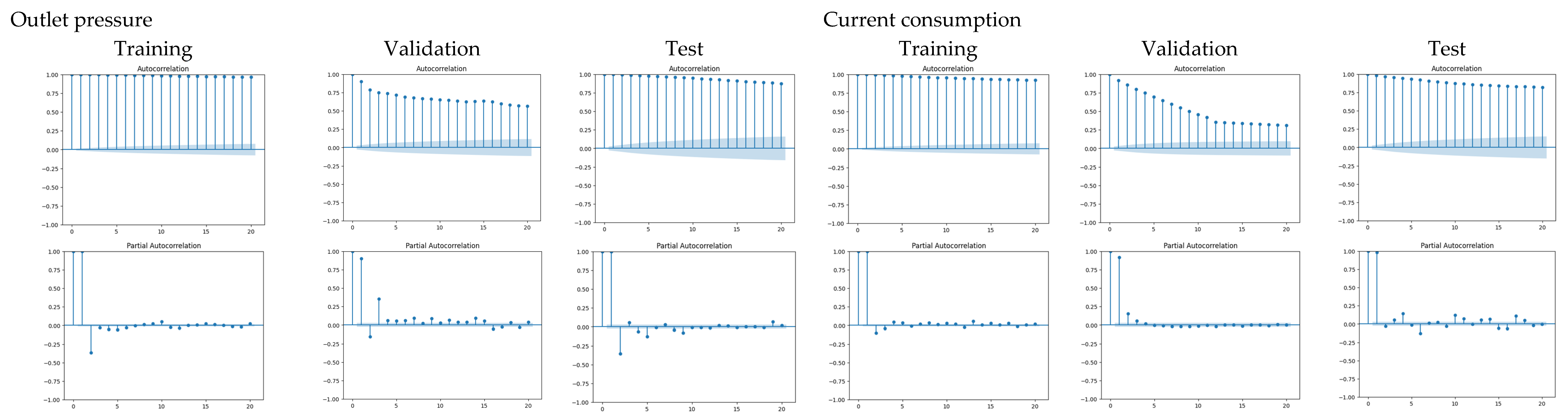
Test	−3.82928	0.002622	Yes

displays the ADF test results for stationarity assessment across the time series, while Figure 9 plots the ACF and PACF used to determine the AR and MA orders.

From Figure 9, the autocorrelation and partial autocorrelation functions indicate the series needs first-order differencing (d = 1), with preliminary evidence supporting at least AR(1) and MA(1) terms in the model specification. The final model corresponds to an ARIMA(1, 1, 2), with the values of statistically significant parameters shown in Figure 10. The values were derived by incrementally testing ARIMA models up to fifth-order terms and retaining only those coefficients that achieved statistical significance (p ≤ 0.05)

The MAE for the training data is 3.4692, which is clearly higher than the values obtained by the neural network (see Table 3). This suggests greater imprecision in the predictions, indicating that the model is unable to capture the underlying patterns of the data and may be experiencing underfitting (an overly simplistic model). Based on the fitted model and using validation data, the residuals exhibit a bias of 0.6007. After bias removal, the percentiles show P_2.5 = −0.4466 and P_97.5 = 0.1741.

Figure 11 depicts the last 1000 test data points, including the forecast limits, control limits, and the prediction provided by the neural network and ARIMAX with bias correction (+0.916 MPa and +0.600 MPa). The evident underfitting of the ARIMAX prediction model manifests in excessively stable forecasts that prove unresponsive to either perturbations or structural changes in the input time series, consequently resulting in increased prediction error. Moreover, a drop in the outlet pressure exceeding the predefined control limits is observed. The primary cause of this issue is a leak in one of the upstream gaskets of the compressor, located between the hydrogen storage tank and the compressor. Although the compressor outlet pressure is successfully regulated, the inlet pressure exhibits erratic behavior characterized by fluctuations and a downward trend.

Several inferences can be drawn from the neural network prediction model. First, the prediction lags delay the actual series. Second, disturbances are smoothed, exhibiting lower amplitude compared to the actual ones. Third, the neural network displays greater variability than the real data, indicating that the network has captured noise during its training and is reflecting it. This highlights the need for further study and a deeper understanding of the process and the current control system.

It can be observed that the control limits estimated by the predictive model are offset relative to the process control limits. Note that the difference between the control limits estimated by the model is slightly smaller than the predefined limits, indicating that the initial issue stems from bias rather than variability (0.945 vs. 1.010 MPa). This bias is attributed to divergent behavior between the validation and test datasets.

The limited dispersion of the original data is likely due to potential over-control by operators on the process (tampering), which must be identified and managed. The causes for this operator behavior, as outlined by [74], are (1) the limited capacity of workers to solve problems and make decisions, (2) differences in each operator’s approach to identifying problems, (3) lack of time and motivation, and (4) shortcuts taken by those responsible for identifying and addressing issues, as there is no record of actions taken on the process

Once the suitability of this technology for predicting future equipment performance has been established, it becomes necessary to incorporate new KPIs into the maintenance plan to monitor emerging technologies and enhance both process sustainability and environmental impact. New KPIs must be implemented to assess maintenance performance, including (1) information and communication technology metrics to evaluate these technological tools’ effectiveness; (2) personnel competency indicators to monitor workforce adaptation to these solutions; and (3) health, safety, and environmental (HSE) measures to enhance organizational sustainability.

7. Critical Discussion

Although the ARIMAX model has demonstrated inferior predictive capability compared to the neural network, it should not be automatically assumed that the latter is devoid of limitations. Deep learning techniques employed in predictive maintenance offer broad applications and future potential, but they face significant challenges in real-world environments—particularly in non-stationary processes. The solution proposed herein encounters the same limitations as those reported by [75,76].

The neural network-based approach presents the following critical limitations:

• Difficulty in failure prediction and/or future asset behavior forecasting, especially under dynamic operational conditions.
• High sensitivity to noisy data.
• Poor transferability/replicability across similar scenarios due to context-dependent learning.
• Dependence on large volumes of labeled data are often impractical in industrial applications.
• High computational demands (e.g., GPU requirements), raising deployment costs.

Beyond technical barriers, organizational and human factors further hinder implementation:

• Resistance to change within traditionally structured organizations.
• Limited awareness among middle and senior management regarding the tools’ capabilities, leading to unrealistic expectations or premature abandonment.
• Black-box nature of the methodology, which undermines trust and decision-making transparency for equipment managers and project leaders.
• Shortage of trained personnel, creating dependency on specialized expertise.

From all the above, the authors consider that the use of this forecasting tool is suitable for supporting the implementation of predictive maintenance, even when dealing with models affected by data noise. It can serve as a starting point to identify the shortcomings of the current system (both technical and organizational) in order to reduce or eliminate them, thereby achieving more accurate results in the future.

8. Conclusions and Future Research

This paper demonstrates that by utilizing existing signals and employing neural networks, redundancy can be achieved, enabling the control of equipment in the event of a communication failure. Furthermore, it illustrates how the use of complex neural networks can predict the actual behavior of a hydrogen compressor and advance maintenance management within organizations. This approach fosters proactivity and predictability, avoiding unnecessary shutdowns, over-costs, the over-control of the process, and the unnecessary use of resources.

Consistent with these findings, this model demonstrates superior generalization capabilities and provides more robust solutions than conventional forecasting systems when faced with pattern shifts in the data series.

The analysis of the neural network has helped to understand and interpret the differing behavior of the process by identifying similarities and/or differences between the validation and test data series. Thus, before implementing complex maintenance plans aimed at deploying actions and tools to enhance the predictive capability of models through the adoption of cyber–physical systems, IoT, security, data storage, etc., it is essential to understand the causes of the compressor’s differing behavior, without overlooking the human factor as a potential source of variability in the process.

The use of predictive models, no matter how complex, enhances the understanding of the process and helps establish action plans focused on efficiently improving the maintenance function. It also increases the sustainability of organizational activities by avoiding the waste of resources on unnecessary actions. However, allowing the system to operate autonomously may lead to undesirable outcomes.

From the study, it can be inferred that the behavior of the original series does not exactly match the predicted series, as the latter exhibits higher variance. Therefore, in the first stage, this information system is intended to be used as an early warning system, since it is likely to produce false positives, not necessarily requiring the controlled shutdown of the equipment.

In the second stage, to improve the model’s predictive capability, adjustments made by control room operators (tampering) on controllable variables will be studied, as these are currently neither analyzed nor recorded, thereby introducing noise into the model.

Once predictive performance is improved (reducing variability), the final stage would involve training neural network-based models that incorporate new (multivariable) inputs, transitioning to condition-based maintenance. This would include analyzing parts wear, asset utilization patterns, and integrating additional sensors into the system.

The scalability of the trained model to other equipment is not anticipated due to the unique nature of the training data, although the same type of neural network architecture with identical hyperparameters may be employed for similar assets.