Different Approaches to Artificial Intelligence–Based Predictive Maintenance on an Axle Test Bench with Highly Varying Tests

Abstract

Maintenance measures are widespread in the industrial environment, and various approaches to maintenance using artificial intelligence are increasingly gaining ground. Predictive assessments of system conditions ensure greater reliability and cost reductions through longer service life. The implementation of a machine learning and a deep learning algorithm for predictive maintenance through early damage detection on an electric rear axle test bench is presented in this paper. The algorithms were selected based on extensive literature research. This paper deals with the question of whether the approach of condition-based or statistical predictive maintenance provides more benefit for a development test bench with highly varying tests. The chosen method of deep learning and machine learning can predict damage for a specific device under test with an accuracy of up to 99% using only one torque signal. In fact, the machine learning approach was found to be sensitive to abnormal behavior on the test bench as well, leaving no abnormality undetected. Although the deep learning model was more resistant to other damage, a pretrained model can be applied to any similar device under test and deliver almost identical results. The methods presented can be adapted to various industrial applications with some adjustments, even without access to big data. This enables predictive maintenance from the very first applications.

1. Introduction

For a durability test bench, reliability and availability are the most important factors for profitable operation. In addition to traditional maintenance, in which systems are operated until they fail or are replaced after a defined service interval, new methods have been developed through the widespread use of artificial intelligence. Predictive maintenance (PdM) can detect failures of both the test bench and the device under test (DUT) in good time, thus predicting abnormalities in the overall system or a component [1].

The question of which systems and components to monitor is inherent in the choice of PdM. While preventive maintenance (PvM) defines fixed replacement intervals for worn parts, it is difficult to prevent sporadic abnormalities. With no known damage to the test bench, it makes sense to shift the focus to monitoring the DUT. Endurance runs on a test bench are carried out until the DUT fails. To derive predictive measures, an assessment of the condition of the DUT is required.

Due to the great attention being paid to PdM, significant progress is being made in terms of implementation [2] and research [3]. Current efforts aim at reducing the cost of PdM systems in industries [4] such as the automotive industry [5] and improving their accuracy through new models and algorithms. This is where the need for big data and real-time models becomes clear [6,7]. PdM methods based on artificial intelligence (AI) are becoming increasingly prevalent and focus on boosting performance and efficiency in PdM [8]. Depending on the problem, the application area, and the available data, machine learning (ML) solves grouping, regression, and classification tasks or is used for anomaly detection. Deep learning (DL) algorithms are used for similar tasks. For optimization, an appropriate algorithm must be selected [9]. Both ML and DL are compared [10] and used particularly frequently in complex and dynamic industrial environments [11].

AI-based techniques, including ML and DL, have been shown in the automotive and manufacturing industries to enhance performance and accuracy in PdM using fault diagnosis [12]. For this, ref. [13] uses intelligent sensors in a smart factory, while [14] uses real-time data from IoT sensors. In addition to optimizing the models and algorithms, it is important to obtain correct features from the input data. Especially for ML, the extracted features play a major role in performance. Some research is therefore aimed at optimizing feature extraction [15].

Although PdM methods can be used almost anywhere, the specific application is important for choosing the right models and algorithms. As an ML method, a support vector machine (SVM) was used in [16] for the classification of a vibration signal of a passenger car. With good results, it was also by far the most frequently used method in a recent research article [17]. For unknown damage cases on an engine with little training data, ref. [18] used a one-class support vector machine (OSVM) to detect abnormalities. Early damage patterns using a vibration signal were recognized in [19,20] with the help of deep learning (DL). In [21], DL was used to monitor the condition of an engine using 21 sensors. In contrast, using only a torque signal, a special type of recurrent neural network (RNN) known as a long-short-term memory (LSTM) network was used to identify faults in a tapping process [22].

With [23] it became clear that SVM and RNN are valid methods for the desired results on a test bench, but it remains unclear how they perform under conditions of constraints and without a controlled test group. In this work, two different AI-based PdM methods were implemented on a rear axle test bench with only limited data available. The main target was to predict damage for highly varying tests to both the test bench and the DUT using a single torque signal and a comparison of different approaches for this purpose. Due to the lack of big data, a condition-based approach was implemented to detect any abnormalities at an early stage. In a statistical approach, trained models were developed based on the measurement data from the first test to help predict identical anomalies in subsequent tests. A series of nine endurance tests reflected the conditions on the test bench and served to verify the selected algorithms.

Section 2 presents the experimental setup with all characteristics and background information on the tests performed. A detailed derivation of the different approaches can be found in Section 3. The input parameters are shown and described together with the software used. In Section 4, results are illustrated, with a comparison of the implemented algorithms and their performance on the test runs. A conclusion in Section 5 highlights the strengths and weaknesses of the methods introduced and how they can be improved and expanded through future work.

2. Electric Rear Axle Test Bench

An electric rear axle test bench (EHAP) was developed and built at the University of Kassel (Department of Mechatronics, with a focus on vehicles). This section presents the test bench’s hardware and software. In addition, a current series of endurance tests is shown. The methods of PdM were implemented based on the framework conditions of this series of tests.

2.1. Structure and Research Environment

The EHAP was designed according to a three-motor concept, i.e., it has one drive motor and two load motors. Each of these motors has a continuous power rating of 550 kW. A DC source with up to 820 V and 1400 A continuous current that powers the axle inverter was used to test electrified axles. Optionally, motor modules with external converters can also be used for axles without vehicle-side inverters. With three gearboxes, maximum speeds of up to 160 km/h and mountain driving can be simulated for each axle type. The structure of a conventional axle on the clamping field is shown in Figure 1a. The structure for an electric axle is shown in Figure 1b.

The research environment of the EHAP covers the drivetrain of transporters weighing 2.8 tons up to heavy trucks weighing over 38 tons. Particularly for electrified axles, approaches for topology concepts arise, i.e., the position, number, and control of the electric machines, and gearbox and gear change investigations [24] with efficiency optimizations of individual components or the overall system are possible. Further test scopes are endurance runs, verification of optimizations, comparison of different performance and efficiency concepts, and load simulations of exceptional driving conditions that are sporadic or difficult to achieve in a vehicle.

A powerful measurement system at the necessary measuring points is essential for achieving the research and testing objectives, as well as for monitoring error-free operation. The use of high-precision torque measurement shafts with an integrated speed/angle of rotation measurement system and other monitoring technology such as current sensors, fault current sensors, vibration technology, and pressure and temperature sensors enable fully automatic operation of the test bench. The EHAP has been certified by TÜV for conformity testing with torque measurement technology directly at the drive or wheel flanges. This includes ECE R 85 [25]. The EHAP is continuously being expanded to include additional measurement technologies so that certifications with increased requirements, such as Annex 10b [26] for new types of axles, can also be fulfilled.

Other components of the EHAP include an oil conditioning system that can permanently regulate the oil sump temperature in the axle housing within a constant temperature range, a water conditioning system that cools the inverters and machines of the electric axle, and a dirty oil cooling system that enables oil tests for endurance tests. In addition, a parameterizable battery simulator can be used for testing the electric drives, which operate under the same voltage–current conditions as the real battery. An illustration of the entire experimental setup is shown in Figure 2.

Fully automated operation of the test bench is made possible, among other things, by self-developed automation software. This also offers the opportunity to implement individual functions, such as controllers or evaluation algorithms. To test these functions, the EHAP has a rapid control prototyping (RCP) environment [27] that accurately models the interaction of a physical test bench model with the real-time software of the test bench.

2.2. Test Execution

The introduction shows that different methods of PdM are being researched. The selection of the best approach depends on the test and its framework conditions. It is also important to determine which measurement signals are best suited for monitoring.

The measurement data of a test series of nine axle differentials are recorded based on a fatigue test in a continuous run. In this case, the device under test (DUT), the test program, and test setup varied to some extent. In addition, defects occurred on the test bench, as well as damage to the DUT. This presents a challenge for finding the appropriate PdM method, but also opens the opportunity to investigate different approaches.

Monitoring, especially of mechanical systems, is carried out via measuring points on or near the critical components. In addition to the generally required speed and torque signals, a powerful industrial vibration sensor including an evaluation unit is available for the test series. The speeds and torques are sampled and recorded at 1 kHz. In contrast, the recorded signal from the vibration sensor is sampled at only 2.63 Hz. This frequency cannot be increased by the internal sensor evaluation unit. This is one of the reasons why the torque signal was chosen as the basis for evaluation. Another reason is provided by the findings of [28,29,30,31]. These state that high-frequency interference with the signal from the vibration sensor can have a negative influence on the evaluation when investigating gear-specific frequencies, such as tooth engagement frequency, which is an optimal indicator of the health of the gearbox.

The recorded torque signal allows tooth engagement frequencies up to the 17th order to be easily recorded and monitored in the speed range driven. In particular, the signal from the torque-measuring shaft on the drive, which is rigidly connected to the differential bevel gear, is well suited for implementing monitoring.

3. AI-Based Early Fault Detection

After the test procedure has been described and the signal used for evaluation has been defined, this section presents the development of the two AI-based methods of predictive maintenance for early damage detection. The procedure for finding an algorithm that matches the problem is then shown step by step. The differences between the two methods are highlighted at the interfaces.

The test series provides the opportunity to implement different types of PdM. Two of these are condition-based and statistical. Condition-based PdM therefore works with sensor data directly from the active test to derive maintenance measures. In contrast, statistical PdM uses historically collected data from series tests and thus draws on experience. In this paper, this definition is extended. Condition-based PdM works with data from the current test and can only derive measures for the same. Statistical PdM can be applied to further tests of the same type after implementation. A model can be trained at the start of the test series and applied to subsequent tests. The use of a pretrained model greatly accelerates evaluation.

Figure 3 shows the selected methods. Only the color-coded paths are discussed in this paper. It is clearly visible which properties and differences arise.

The red path leads to the development of an anomaly detection system for condition-based PdM using machine learning (ML). A special type of one-class support vector machine (OSVM) is to be used for this purpose. The blue path runs through statistical PdM. Using deep learning (DL), a classification task is to be solved by an artificial neural network (ANN). For this purpose, a long short-term memory (LSTM) network is selected, which can be assigned to recurrent neural networks (RNN). As shown, AI is the overarching concept for ML, of which DL is a subfield. It is possible to implement these methods directly in MATLAB 2022b, which was used in this work. This simplifies application to a specifically defined problem, and, in addition, the measurement data are already available in MATLAB and do not have to be converted from other data formats before evaluation. The two selected methods are presented in detail below.

3.1. One-Class Support Vector Machine (ML)

SVM is a proven method for solving classification tasks [32]. One variant of this, which is particularly suitable for condition-based PdM, is OSVM. It requires only one data class for classification or for the detection of an anomaly. This is usually the class whose data are generated at the beginning of the inspection and are marked as “normal”. To do this, it is necessary to identify in advance which features are suitable for differentiating between “normal” data and an anomaly.

As previously outlined in the test procedure, the specific frequencies of the gears, including the tooth mesh $f_{\mathrm{z}}$, the first side bands of the bevel gear $f_{\mathrm{z}}\pm f_1$, and the first and second side bands of the disk gear $f_{\mathrm{z}}\pm f_2$ and $f_{\mathrm{z}}\pm 2f_2$ can be used to make reasonable estimates about the condition of the differential. This is based on the frequencies

$$f_1={\displaystyle \frac{n}{60\mathrm{s}}}$$

(1)

and

$$f_2={\displaystyle \frac{n}{60\mathrm{s}}}·{\displaystyle \frac{1}{i}}$$

(2)

at a specific speed n in rpm and transmission ratio i. While damage to a single tooth (local) is more likely to be noticeable through an increase in the amplitude of the sidebands [33], damage to all teeth (circumferential), such as abrasive wear or scuffing, can be recognized by an increase in the amplitude of the tooth mesh frequency. This results in seven features that are extracted from the torque signal of the drive, which are explicitly defined in

Table 1. Features extracted from torque sequences in the frequency range at a constant drive speed of 1584 rpm with a gear ratio of $i={\displaystyle \frac{31}{15}}$.

Feature	Value (Hz)
$f_{\mathrm{z}}$	396
$f_{\mathrm{z}}+f_1$	422.4
$f_{\mathrm{z}}-f_1$	369.6
$f_{\mathrm{z}}+f_2$	408.8
$f_{\mathrm{z}}-f_2$	383.2
$f_{\mathrm{z}}+2f_2$	421.6
$f_{\mathrm{z}}-2f_2$	370.4

. MATLAB offers the option of doing this via the Diagnostic Feature Designer App. Before the values of the features are determined, the most frequently used operating point from the test run is selected for a comparable analysis. Here, this operating point has a constant torque of 500 Nm and a constant speed of 1584 rpm. This eliminates speed- and torque-dependent changes in gear-specific frequencies. In addition, the torque signal used is divided into sequences of equal length. This results in six sequences of a fixed length of 2000 data points per run in the test program used. The features values are extracted from these sequences and assigned to the test run together. The spectral power density is formed using Wel’s method [34] to determine the feature value from the torque sequences. This method can be used to clearly determine all the named features from the torque signal.

The basic idea of SVM is the identification of an optimal separating line or plane between two classes. In the context of a data set

$$\left(x_1,y_1\right),\left(x_2,y_2\right),\dots ,\left(x_{\mathrm{n}},y_{\mathrm{n}}\right)$$

(3)

comprising a feature vector $x_iϵ{\mathbb{R}}^d$ of the $i$-th data point in dimension $d$ and a class label $y_iϵ\left\{-\mathrm{1,1}\right\}$ the separating plane can be described by

$$w·x+b=0$$

(4)

where $w$ represents the vector of weights and $b$ denotes the bias, which indicates the distance from the origin to the separating plane. The optimization problem of the SVM

$${min}_{w,b}{\displaystyle \frac{1}{2}}{‖w‖}^2$$

(5)

with the constraint

$$y_i\left(w{·x}_i+b\right)\ge 1,{\forall }_i$$

(6)

is to identify the maximum distance of the separating plane to the nearest data points.

While SVMs separate two classes, OSVM learns a decision function that describes the largest possible part of the trained class in a space. It identifies outliers from this as anomalies. Since no class labels are used for this, this method is unsupervised learning. This is sometimes also referred to as semi-supervised learning, since the class of the trained data is named. The new function of the separating plane $f\left(x\right)=w·\varphi \left(x\right)-\rho =0$ is obtained, where $\varphi \left(x\right)$ is a mapping into a higher-dimensional space, and $\rho$ is a threshold value. This results in an optimization problem that is expressed as

$${min}_{w,\rho }{\displaystyle \frac{1}{2}}{‖w‖}^2$$

(7)

with the constraint

$$\left(w{·\varphi (x}_i)\right)\ge \rho ,{\forall }_i$$

(8)

By solving this problem, the OSVM can recognize data outside the trained space as an anomaly. This approach yields favorable results for instances where the nature of the error is not known in advance and may affect the data in various ways.

For implementation in MATLAB, the seven features from the torque signal at a constant operating point are extracted as described above using the Diagnostics Feature Designer App in MATLAB. The feature values obtained in this way are used to train an SVM model using the fitcsvm function with the input parameter from

Table 2. Input parameter values of the fitcsvm function to train the SVM model.

Parameter	Value
Table—Sample Data	Extracted feature data
Label	“normal”
Outlier Fraction	0.00
Standardize	“true”
Kernel Scale	“auto”

. The measured values are standardized before being transferred and assigned the label of their class. It is assumed that the measurement data do not contain any outliers. The result is a trained SVM model that can recognize anomalies in the measurement data.

There are several graphical tools for displaying the quality of the trained model, including the frequency distribution as a confusion matrix. Figure 4 shows the confusion matrix of the anomaly detection of the OSVM, which was trained using data from the first test and then applied to run 30, which contains measurement data from the normal state, and run 460, in which the differential is barely operational and exhibits abnormal behavior, of the same test. It can be seen that normal data were recognized as normal, with a probability of 100%. Anomalies were recognized as abnormal, with 100% probability. This means that the algorithm can differentiate normal from abnormal data with absolute certainty. Misclassifications, which indicate uncertainties in the model, are not present for these two runs.

3.2. Recurrent Neural Network: Long Short-Term Memory (DL)

Another approach to implementing a predictive maintenance method using artificial intelligence is to use deep learning (DL). The use of artificial neural networks (ANNs) is significantly more complex in structure than the ML approach.

Artificial neural networks consist of individual neurons organized in layers. These include an input layer, hidden layers, and an output layer. An input signal thus passes through each neuron, is weighted, and is output as a result. The result is generated by activation functions. The extent to which DL can work is demonstrated by the Universal Approximation Theorem [35]. This states that a feed-forward network with only one hidden layer and a sufficient number of neurons is able to approximate any continuous function with arbitrary accuracy. However, this capability is inherently linked to the complexity of the data. It should also be noted that the No Free Lunch Theorem (NFLT) [36] states that no algorithm is good for all optimization problems. Any algorithm developed for one problem may therefore be poorly suited to other tasks.

Recurrent neural networks (RNNs) are a type of neural network (NN) that are used specifically for processing sequential data. They possess a feedback loop that enables them to retain information from previous sample points. From a mathematical perspective, an RNN can be represented by

$$h_{\mathrm{t}}=f(W_{\mathrm{h}\mathrm{x}}{x}_{\mathrm{t}}+W_{\mathrm{h}\mathrm{h}}{h}_{\mathrm{t}-1}+b_{\mathrm{h}})$$

(9)

with the output vector

$$y_{\mathrm{t}}=W_{\mathrm{h}\mathrm{y}}{h}_{\mathrm{t}}+b_{\mathrm{y}}$$

(10)

and the state $h_t$ at time $t$, the input vector $x_t$, the weighting matrix $W$, and the bias $b$ [37].

A specific type of recurrent neural network (RNN) is the long short-term memory (LSTM) network. This was created with the objective of more effectively learning long-term dependencies in time signals. In comparison to standard RNNs, it possesses a form of memory function. Specialized gates within the network’s structure store pertinent information over extended periods of time and delete irrelevant information, which is essential for effective learning from intricate time signals. The gates are constructed differently and utilize the sigmoid function $\sigma$ or the hyperbolic function $tanh$ as an activation term. The input gate $i_t$, the forget gate $f_t$, and the output gate $o_t$ determine which information from the previous state is passed on to the next. The change of state through the gates can be described mathematically, as in [38]:

$$i_{\mathrm{t}}=\sigma (W_i·\left[h_{\mathrm{t}-1},x_{\mathrm{t}}\right]+b_i)$$

(11)

$$f_{\mathrm{t}}=\sigma (W_f·\left[h_{\mathrm{t}-1},x_{\mathrm{t}}\right]+b_f)$$

(12)

$$o_{\mathrm{t}}=\sigma (W_o·\left[h_{\mathrm{t}-1},x_{\mathrm{t}}\right]+b_o)$$

(13)

$${\tilde{C}}_{\mathrm{t}}=tanh(W_C·\left[h_{\mathrm{t}-1},x_{\mathrm{t}}\right]+b_C)$$

(14)

$$C_{\mathrm{t}}=f_{\mathrm{t}}\ast C_{\mathrm{t}-1}+i_{\mathrm{t}}\ast {\tilde{C}}_t$$

(15)

$$h_{\mathrm{t}}=o_{\mathrm{t}}\ast \mathrm{t}\mathrm{a}\mathrm{n}\mathrm{h}\left(C_{\mathrm{t}}\right)$$

(16)

The NN can be assembled with individual layers in the MATLAB app Deep Network Designer. In this work, an RNN with six sequentially connected layers is used. It consists chronologically of the input layer, lstmLayer, dropoutLayer, fullyconnectedLayer, softmaxLayer, and classificationLayer. The function of the individual layers can be found in the MATLAB documentation. Some of these layers can also be parameterized. Various options can also be selected for the subsequent training process of the LSTM network.

Table 3. Input parameter values of the layers for the LSTM network.

Layer	Parameter	Value
InputLayer	Inputsize	1
lstmLayer	Numhiddenunits	14
dropoutLayer	Probability	0.3
FullyConnectedLayer	Outputsize	2

shows the parameters of the layers used here, and

Table 4. Training options for the LSTM network.

Parameter	Value
Solver	Adam
MaxEpochs	3
InitialLearnRate	0.001
LearnRateDropFactor	0.2
MiniBatchSize	128
ValidationFrequency	20

shows the settings for training the LSTM network.

In comparison to the OSVM, the torque sequences must be reduced from 2000 to 100 data points. No result could be achieved with 2000 data points. Therefore, more but shorter sequences are used as input. Another important aspect is that the LSTM network selects features independently. Before the data are used, they are additionally normalized and shuffled to prevent the LSTM network from drawing conclusions about the order of the input.

After the detailed introduction to the LSTM network used and the training process, Figure 5 shows the confusion matrix of classification by the LSTM network. It was trained using data from the first test and then applied to run 30 and run 460. The matrix shows that the network is very well suited for this classification task. It makes correct predictions for the normal class, with a high probability of 99.8%, and for the abnormal class, with a probability of 99.9%.

4. Results

After the selection process and the implementation of the two methods of predictive maintenance have been described, the first results are presented and evaluated in this section. In the current development phase, each method is always applied to a completed measurement data set. This means that the evaluation takes place after each run. The results always show an entire endurance run, from the start to the point at which the device under test (DUT) could no longer be operated due to damage.

The statistical instrument of the empirical probability $h_{\mathrm{n}}$ is introduced to represent the results. The empirical probability

$$h_{\mathrm{n}}\left(A\right)={\displaystyle \frac{H_{\mathrm{n}}\left(A\right)}{n}}$$

(17)

with respect to the event A of a data sequence classified as abnormal is defined as the quotient of the absolute probability $H_{\mathrm{n}}$ and the number n of observed elements of a set. This indicates that, for $h_{\mathrm{n}}\left(A\right)=0$, each observed sequence n in the run N was classified as normal. Consequently, for $h_{\mathrm{n}}\left(A\right)=1$, each observed sequence is classified abnormal. On average, 215 data sequences with 2000 data points per run for the OSVM and 4300 data sequences with 100 data points per run for the LSTM were used to calculate the empirical probability. The empirical probability is a particularly good parameter to show the increase of abnormal data within many consecutive runs.

The results of the first, fourth, seventh, and ninth DUT are presented and compared from the test series. All other results are similar. The exact times at which, for example, a tooth broke are not known. The tests were each ended after a further operation was no longer possible due to excessive vibration or temperature values.

4.1. One-Class Support Vector Machine (ML)

The results of the OSVM presented are shown below. The empirical probability determined from Equation (17) is listed over the number N of runs of the target value profile driven. Runs 30–40 are used for training or for the specification of normally classified torque sequences. The basis for this is the check in Figure 6. The first runs are not well suited, due to run-in processes. This was checked using runs 0–10, 10–20, and 20–30. Later runs (>40) should not be used, as otherwise the first signs of wear could be taught in.

In addition, a distinction was made in the anomaly detection of the OSVM between damage to a single tooth (local) and to all the teeth of the gear (circular). Furthermore, the trained models are also tested on other DUTs, i.e., the method is also used as a statistical PdM. The results of the inspection for circular tooth damage are shown below, followed by those for local tooth damage.

In Figure 7, the OSVM results series shows that, for each test, a model for rotating gear damage, i.e., including all seven features, was trained and applied to the test in question. As already mentioned in Section 2.2, there were several incidents during the tests that are explained in connection with the results.

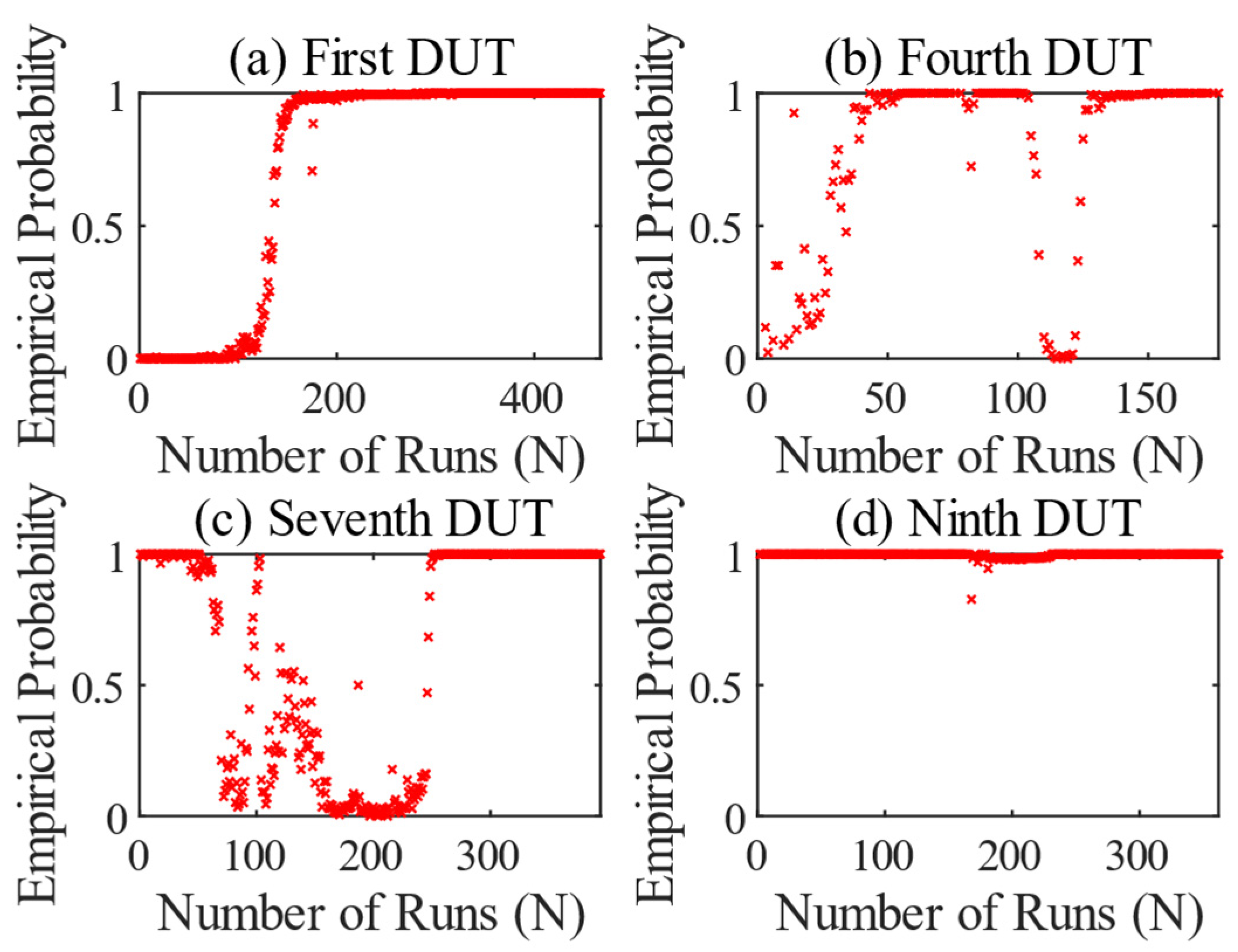
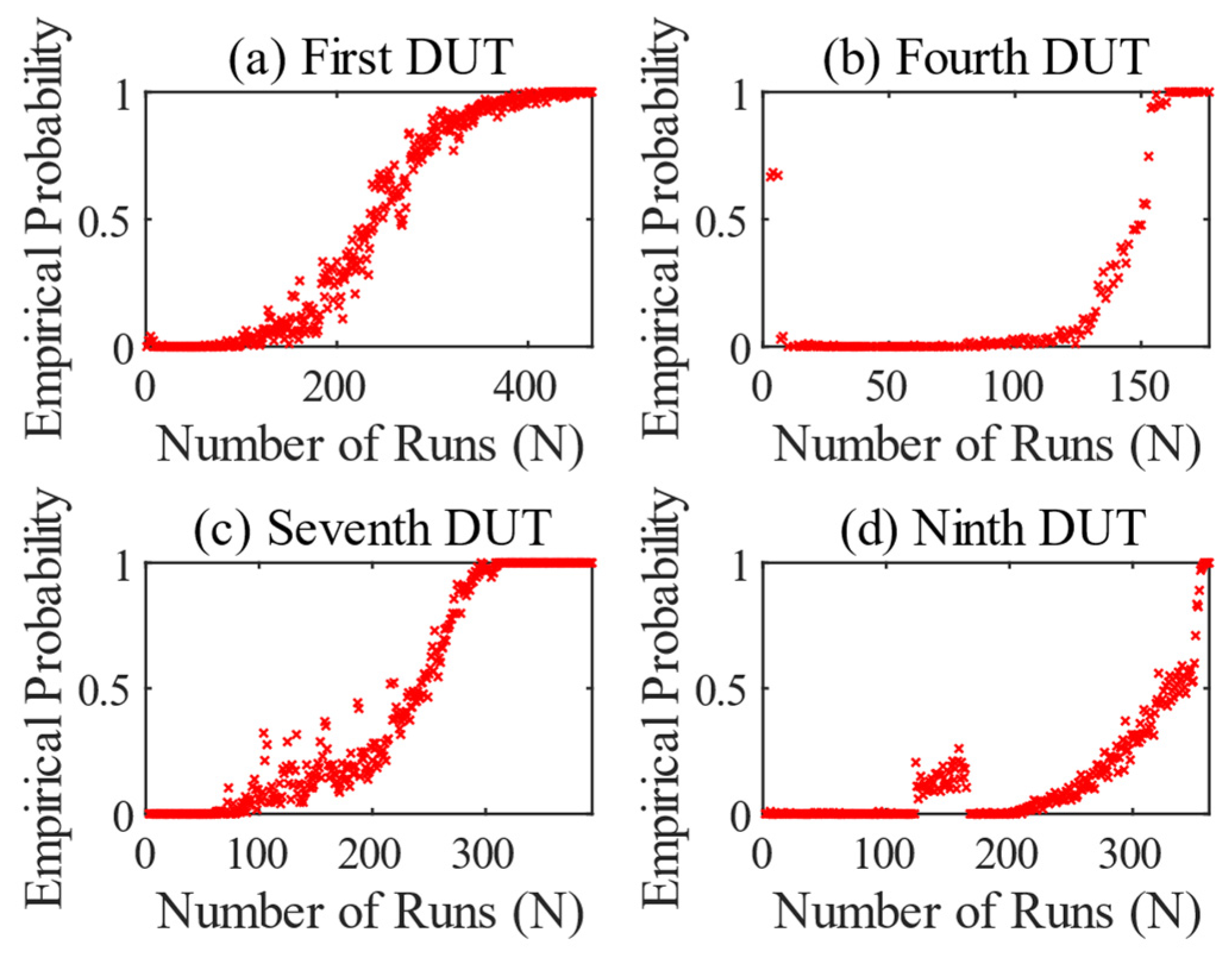
The result of the first DUT is shown in Figure 7a. The test ran normally and without any special incidents. From run 95 onwards, the OSVM begins to recognize an anomaly or a change in the specific features of the gearbox. From that point on, the empirical probability increases permanently. From run 215 onwards, the values are permanently 1, except for two outliers. However, the DUT did not fail until run number 465. This means that the method recognizes an anomaly at an early stage. Or, to put it another way, the anomaly that is recognized is an early sign of wear.

The test of the fourth DUT in Figure 7b shows abnormal behavior at the beginning of the test, which quickly changes to a normal state. This may be due to changes in the gearbox caused by the running-in process. From run 50 onwards, the vibration values on the DUT increased. At this point, the side shafts of the differential had to be replaced due to abnormality. This meant that the empirical probability remained at 1 for the rest of the test. The test was terminated after the 177th run. The differential showed heavy pitting and bearing damage. The replacement of the side shafts led to a change in the monitored features, and thus to abnormal behavior, which caused the anomaly detection to fail.

Figure 7c shows the result for the seventh DUT, which behaves in a similar way to the first DUT. However, an anomaly appears in run 90, which initially disappears again. This can be seen from the steep increase in the empirical probability and the subsequent abrupt drop. From run 110 onwards, the value increases continuously and then remains at 1. In the context of the test procedure, the first anomaly detected is associated with impending breakage of a gearbox mounting of the DUT. To generate such a deflection, the resulting vibration must have been superimposed on the frequency of the gear-specific features. In run 103, this mounting was torn off and repaired. This resulted in elimination of the anomaly. Furthermore, wear in the differential is also identified as an anomaly here. The DUT failed from run 394.

The inspection of the ninth differential in Figure 7d behaved similarly. From run 124, a kind of clustering occurs over 40 runs, after which the empirical probability breaks out and rises continuously until it stabilizes at 1 from run 185. Again, the wear was recognized as an anomaly. The DUT failed from run 362 and could no longer be operated. It is interesting to note in the context of the test that an abnormal bellows on the drive had to be replaced after run 165. After the replacement, the clustering ended. Here too, the PdM provided an indication of abnormal behavior of the test bench, which had a slight influence on the extracted features of the DUT.

Figure 8 shows the results of the OSVM when a model for circumferential gear damage was trained using the first test. This model is then applied to the data from the other tests. The results of the first test in Figure 7a and Figure 8a are therefore identical. No good results are generated for the other tests in Figure 8b–d. Although the values are in the correct range towards the end of the tests, the behavior of the DUTs in the normal state appears to differ. This leads to anomalies being identified at the beginning. In some cases, these disappear again due to the factors mentioned, such as running-in processes or repairs of abnormal components on the test bench.

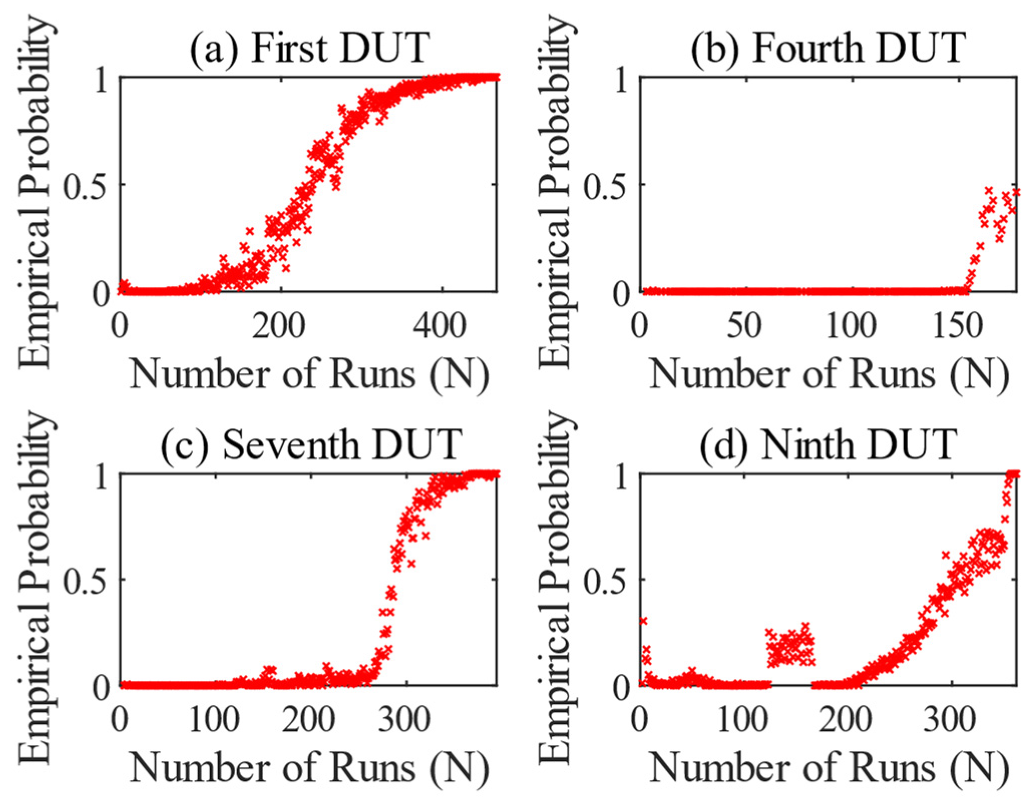
Figure 9 shows the results of the OSVM, where a model for local gear damage, i.e., in terms of the features $f_{\mathrm{z}}\pm f_2$ and $f_{\mathrm{z}}\pm 2f_2$, was trained for each test and applied to the test in question. The results in Figure 9 differ in principle from those of the circumferential tooth damage, as they only increase at a later stage. This is in line with the theory of tooth damage. The empirical probability in Figure 9a increases gradually from run 150 onwards, as in the previous test, because wear can also affect the side bands, but not to the same extent as local damage. The value then increases steadily until it reaches 1 for the first time from run 405 onwards. After that, the empirical probability remains in this range until the end of the test.

The test of the fourth DUT in Figure 9b again shows a strong run-in process, but then normal operating behavior for a long time. The change of the side shafts in run 50 has no influence on the monitored features of the local tooth damage. After 125 runs, the empirical probability then begins to rise and reaches a value of 1 after 25 more runs. The reason for the failure is not fully clear, but a combination of heavy pitting and bearing damage in the differential was observed. The result of the OSVM indicates abnormal behavior regarding the monitored features at the end of the test.

The result in Figure 9c shows the same behavior as in Figure 9a. It is noticeable that the anomaly described in Figure 7c, where a mounting has come loose, is not recognizable. The external influences therefore had a greater effect on the tooth engagement frequency, which was not taken into account here. In contrast, examination of the data from the ninth test in Figure 9d shows similar clustering, as previously described in Figure 7d. An abnormal bellows stimulated the system in such a way that abnormal behavior was registered. In addition, the way in which the empirical probability develops towards the end is different. In comparison to the results of the first and seventh tests, which show a slowing increase, the progression here from run 350 onwards is more like exponential growth. Only the last eight runs have a value around 1.

The OSVM results in Figure 10 show the use of the model trained on the first test run, in relation to the features $f_{\mathrm{z}}\pm f_2$ and $f_{\mathrm{z}}\pm 2f_2$, which was applied to the other tests. The graphs in Figure 9a and Figure 10a are therefore identical. While the model trained on the fourth test in Figure 9b already indicates an anomaly at run 150, the empirical probability in Figure 10b is still 0 at run 150. The model trained on the first DUT obviously requires more strongly increasing amplitudes of the monitored frequencies for an increase in the empirical probability. Likewise, the increase only reaches a value of 0.5 towards the end of the test. With the knowledge that the differential failed with heavy pitting and without tooth breakage, this result is conclusive.

When looking at the results of the two seventh DUTs, it is noticeable that the foreign model used probably experienced higher feature values earlier. This delays the increase in the graph, but otherwise behaves the same. Figure 10d only shows increased scatter at the beginning and around run 330 in comparison to Figure 9d. Compared to the circumferential gear damage, a previously trained model can therefore be applied to further tests. This means that both condition-based and statistical PdM are possible with OSVM.

4.2. Recurrent Neural Network: Long Short-Term Memory (DL)

The results of the DL method of predictive maintenance are also presented by calculating the empirical probability from Equation (17).

Again, it is checked which runs are best suited for training normal data. For a classification task, it may be useful to use the same number of data sequences for both classes for training. For this reason, the last ten runs before the failure of the differential are used as abnormal data for the training process. Regarding the data of the abnormal class, this means that the LSTM network is trained on local tooth damage or heavy wear. Figure 11 shows the results of the 1st DUT of the LSTM network. The runs used to train the network will have a slight influence on the result. Considering the running-in behavior and the occurrence of initial signs of wear, runs 30–40 are again selected for training.

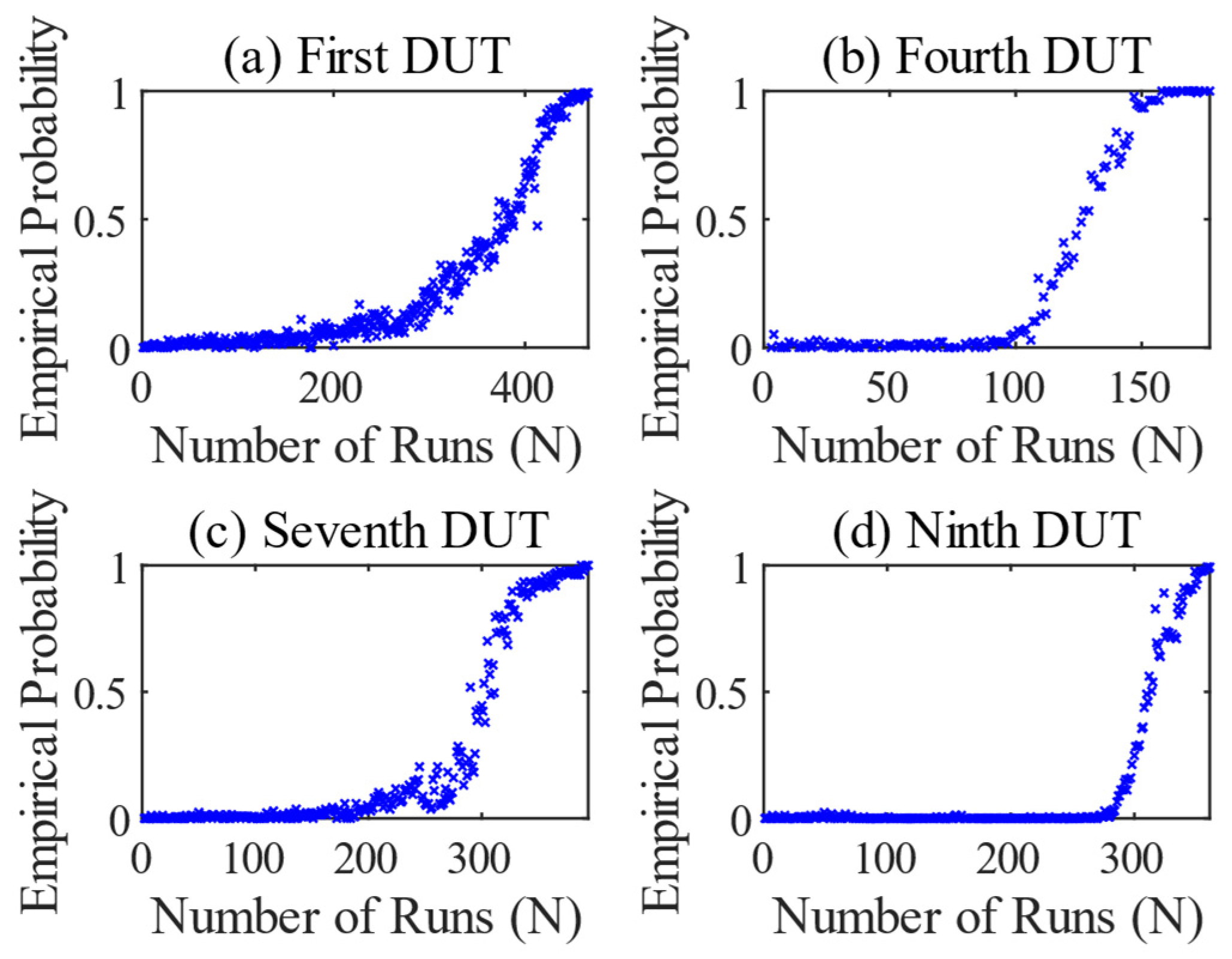
Figure 12 shows the result series of the LSTM network classification, in which a model was trained for each DUT and applied to its own test. The result of the first DUT is shown in Figure 12a. The empirical probability starts to increase from run 305 onwards, indicating a change in transmission. From there on, the torque sequences are no longer classified as normal. From run 450 on, the values are permanently in the range around 1. The method fulfills the classification task exactly as it was designed and recognizes the abnormal data sequences for the last runs. Early signs of wear are irrelevant to the LSTM network and are of little consequence. The results of the other tests are similarly good. In Figure 12b–d, the values rise continuously towards the end and reach an empirical probability of 1 shortly before the DUTs fails. The LSTM network does not provide any indications of abnormal components on the test bench, as the OSVM does. Another special feature is that the fourth test in Figure 12b was taught to recognize a combinatorial abnormality with damage to the gears and bearings. Here too, the LSTM network finds a good solution for the classification task of distinguishing the features in the measured values.

Figure 13 shows the results when a model trained on the first DUT is applied to the other tests, which follows the approach of statistical PdM. Graphs (a) and (c) in Figure 12 and Figure 13 show a high degree of correlation. The visible difference in (b) is because the model of the first DUT was trained on a missing tooth. When applied to the measurement data from the fourth test, in which no tooth was missing, the empirical probability in Figure 13b does not reach a value of 1 at the end of the test. The result of the ninth test in Figure 13d differs greatly from the condition-based PdM approach in Figure 12d. Obviously, the data at the beginning are too different to use the model of the first DUT. The behavior of the graph only normalizes from run 165 onwards. This is where the abnormal bellows was replaced. After that, the values of the empirical probability slowly increase with an increased spread and reach values around 1 from run 300 on.

4.3. Comparison

The stated aim of this study is to find an approach that produces good results with a high degree of accuracy, even with highly varying test runs. Both methods have undeniable advantages for this purpose.

In addition to the results shown, the duration of the calculation is an important criterion for evaluating the PdM methods. For this purpose, a timer was integrated into the scripts for training and evaluation to output the calculation times.

Table 5. Runtime calculation of the evaluation of the OSVM for a model that has already been trained and without a pretrained model. Features used for (a) circumferential and (b) local tooth damage.

Features Used	DUT (N)	Pretrained Model Available	No Pretrained Model Available
(a) circumferential	1 (468)	6.46 s (1924.80 s)	49.67 s (2006.87 s)
	4 (177)	5.44 s (839.58 s)	56.29 s (901.95 s)
	7 (394)	5.69 s (1491.34 s)	63.46 s (1615.78 s)
	9 (362)	6.32 s (1913.35 s)	68.66 s (2060.19 s)
(b) local tooth damage	1 (468)	5.9 s (2088.43 s)	72.97 s (2356.98 s)
	4 (177)	5.72 s (833.16 s)	57.97 s (890.54 s)
	7 (394)	6.33 s (1549.91 s)	67.01 s (1722.27 s)
	9 (362)	6.6 s (1882.23 s)	64.23 s (1981.91 s)

shows the calculation duration for the empirical probability of the OSVM of the respective tests. To better understand the influence on this, various factors are investigated. On the one hand, the effect of an already pretrained model is examined, which shows how long the evaluation, including the training process, takes. In addition, the weighting of the number of runs and features tested is also analyzed. To do this, the calculation for one run is shown, and the calculation time for all runs of the respective test is given in brackets. The table shows that, for the OSVM, a pretrained model reduces the calculation time slightly, especially when only a few runs are evaluated, as in this case, for example, which had only one run. There is almost no difference between the number of features used.

Equivalent to Table 5, a runtime calculation was made for the DL method. As can be seen in

Table 6. Runtime calculation of the evaluation of the LSTM network for a model that has already been trained and without a pretrained model.

DUT (N)	Pretrained Model Available	No Pretrained Model Available
1 (468)	0.86 s (126.19 s)	60.15 s (214.60 s)
4 (177)	0.78 s (68.44 s)	89.04 s (223.86 s)
7 (394)	0.94 s (109.05 s)	81.75 s (199.57 s)
9 (362)	0.95 s (119.78 s)	92.82 s (188.21 s)

, the times for a single run and for all runs of a test are determined with and without a pretrained model. Despite the complexity of the RNN structure, the statement on the condition of the DUT of a single run is calculated in less than a second. In direct comparison, it is therefore significantly faster than the OSVM. When it comes to calculating the data for an entire test, evaluation with a pretrained LSTM network is up to twenty times faster.

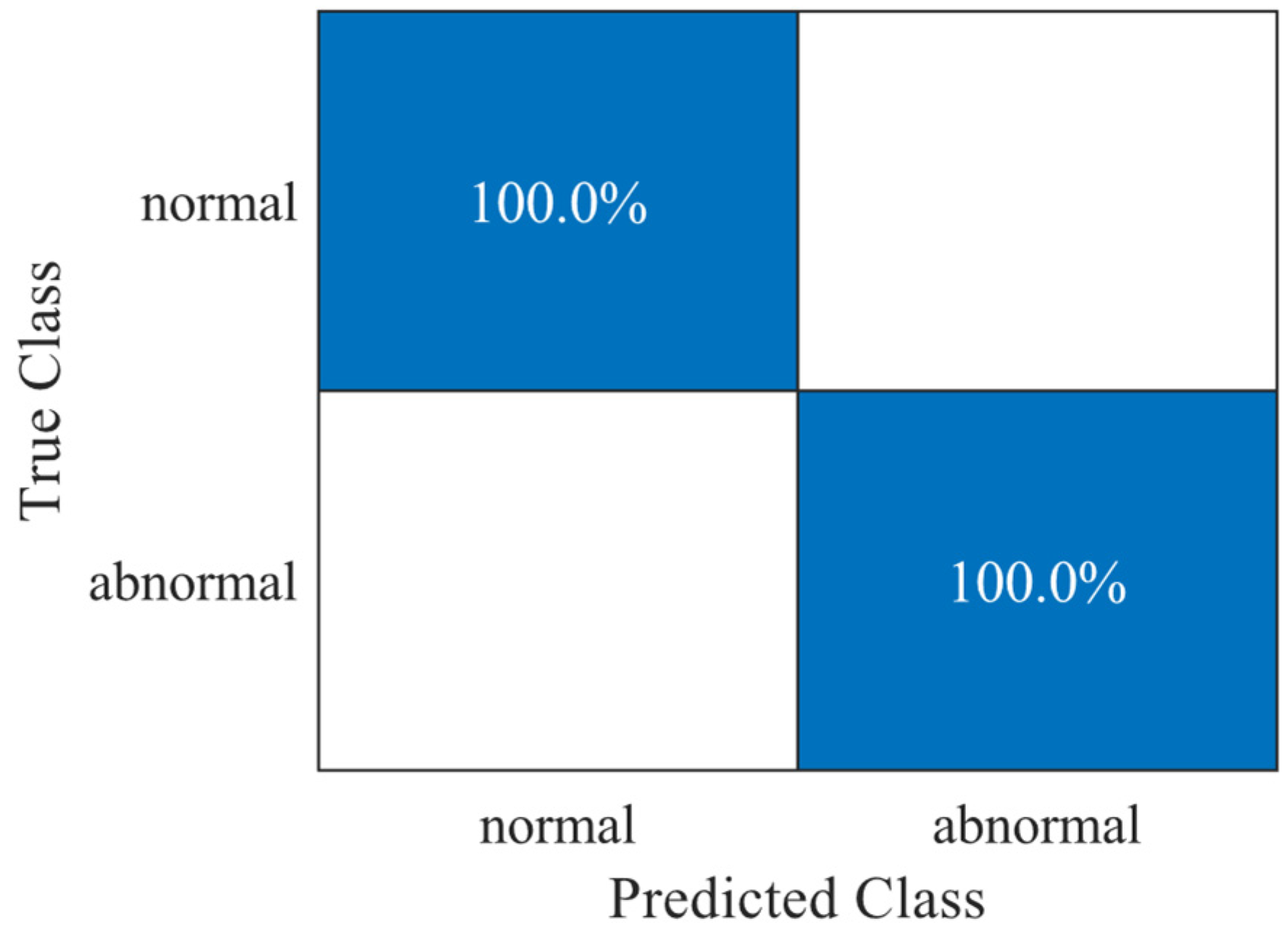
It is difficult to determine the accuracy of OSVM in detecting anomalies, as it uses semi-supervised learning where no data are labeled as “abnormal” and therefore cannot be used to validate the results. The anomalies detected in the tests can be marked for subsequent evaluation. Figure 4 shows that normal data can be clearly distinguished from abnormal data. Other anomalies, such as damaged components of the test bench, also resulted in a detected anomaly. Of the nine test runs carried out, it can generally be said that no anomaly remained undetected.

The validation accuracy and the loss for the trained LSTM networks for the respective tests are determined in

Table 7. Validation accuracy and loss of the trained LSTM networks of the associated tests.

DUT (N)	Validation Accuracy	Validation Loss	Value
1 (468)	99.82%	0.0213	1
4 (177)	99.81%	0.0292	14
7 (394)	99.02%	0.0339	2
9 (362)	99.98%	0.0009	0.3

. To calculate the accuracy, the trained model is applied to its own mixed data set, which contains a label of the actual class. The loss is formed by cross entropy of the predicted and the actual class and should be minimized in the training process. Both the high accuracy of over 99% and the low loss show that the trained models work with great precision.

5. Conclusions

The results show that the selected PdM methods are meaningful in the EHAP. During the test series, they were able to contribute to a better assessment of wear behavior and estimate the condition of the axle. Despite the limitations that the test runs have high variability and that no exact damage cases could be defined in the data, such as a missing tooth on the bevel gear, the results are satisfactory.

The OSVM is very reliable at finding anomalies. No anomaly remained undetected, so damage to the test bench and DUT could be responded to at an early stage. For the approach of specifically identifying a broken tooth, the ML method was redesigned to detect local tooth damage. In this design, the method can be used with both condition-based and statistical PdM. For circumferential tooth damage, initial signs of wear such as pitting, or even abnormal test bench components, were classified as abnormal using all seven features. However, when a pretrained model is used for circumferential tooth damage, it is not robust enough to be applied to similar DUTs. Another reason for this can be overfitting, which means that too many features have been used that negatively influence the result. In this case, it can only be used as condition-based PdM.

The LSTM network is trained on a heavily worn differential, some of which have tooth damage, and reliably recognizes comparable conditions even in other DUTs. The selected deep learning method showed no reaction to the developing damage on the test bench. This suggests that it can distinguish the DUT well from the overall system. To detect the occurred damage to the test bench, it must be trained for these cases and their effects on the torque signal.

With an outstanding performance of over 99%, the LSTM network solves the classification task between normal and abnormal data, as shown in Table 7. The performance of the ML and DL algorithms differs also in terms of calculation time, with various factors being considered. For existing trained models, a calculation time of approx. 7 s after a run is sufficiently fast to be able to intervene in the event of damage being detected. To make both methods suitable for further implementation in the automation software to perform online evaluation, the calculation time must be reduced to meet real-time requirements. One possible approach to achieve this is to reduce the number of data sequences used per run. By halving the number, the calculation time could be reduced by 20% for DL and by 50% for ML. A greater reduction and the influence on the result must be investigated further.

In addition to the certification measurements, further endurance tests for other DUTs will be carried out on the EHAP. The tests described here show that the conditions in a test series are unlikely to be identical. In addition, damage events cannot be clearly defined and sometimes occur simultaneously. For these tests, the aim should be to focus more on condition-based PdM as an anomaly detection and optimize it. The same applies to individual tests and monitoring of test bench components.

Artificially generated measurement data can be used to reinforce data. In this case, approaches for improving the PdM methods can be implemented either completely from artificial measurement data or as hybrid data sets. The creation of artificial measurement data can be either theory-based or experience-based. It is even possible to overcome data limitations using generative AI. Handling artificial measurement data can also have disadvantages such as overfitting. Precise validation of generation of artificial measurement data must be carried out before it is used further. The described procedures can be also incorporated into a Digital Twin [39]. Further improvements for the training process and for strengthening the results can be cross-DUT learning techniques or adding more inputs like a vibration signal to the algorithms.