Explicit Time Integration Method Based on Uniform Trigonometric B-Spline Function for Transient Heat Conduction Analysis

Abstract

In this paper, a new explicit time integration method for transient heat conduction analysis is proposed based on the uniform trigonometric B-spline function. The algorithmic calculation procedure for solving the heat conduction problem is given. The influence of algorithm parameters on accuracy and stability is determined by theoretical analysis and numerical experiments. With adjustable parameters, the proposed method can obtain high-order calculation accuracy and a large stability region. The local truncation error analysis of transient heat conduction shows that the proposed method has at least second-order accuracy. The numerical examples verify the effectiveness of the proposed method for linear and nonlinear heat conduction problems.

1. Introduction

Transient heat conduction phenomena are common in engineering fields, such as aerospace, metallurgy, and civil engineering. Analytical solutions are only available for linear problems with simple geometries, and experimental solutions are usually difficult to obtain for some complex heat conduction problems. The numerical method is a powerful tool to solve the transient heat conduction problem effectively.

Accurate modeling and efficient simulation are necessary for transient heat conduction. Thus, various numerical methods have been developed over the last several decades, including the finite difference method (FDM) [1,2], the finite element method (FEM) [3,4], and the meshless methods [5]. Currently, the FEM is most widely used for spatial discretization, and direct time integration is usually used for temporal discretization in numerical simulation [6].

In general, direct time integration methods can be majorly categorized into explicit and implicit methods [7]. There are some classical implicit methods, such as the backward Euler method, the Crank–Nicolson method [8], the Newmark method [9], and the generalized-α method [10]. These methods are generally unconditionally stable, allowing for large time steps in long-term simulations. However, the implicit methods often require a much larger computational effort per time step than the explicit methods [10]. The traditional explicit methods, such as the forward Euler method, the central difference method, and the Runge–Kutta method, have a simple computational formulation and high per-step efficiency [7]. However, they are conditionally stable. A small time step must be chosen in the calculation, which limits its application in long-term transient heat conduction problems. In short, various methods have their advantages and disadvantages; more detailed discussion can be found in Ref [7,11]. This paper focuses on the explicit method.

In fact, the choice of direct time integration method significantly determines computation efficiency and accuracy. As the demand for higher efficiency and accuracy increases, advanced explicit time integration methods with desirable algorithmic properties continue to emerge [12,13]. Many explicit methods with numerical dissipation characteristics have been proposed, such as the Zhai method [14], the HC method [15], the TW method [16], and the Soares method [17]. Among them, although the TW method has only first-order accuracy, its accuracy is sometimes higher than those of some second-order methods for calculation in low-frequency modes. The explicit method proposed by Noh and Bathe [6] (called the Noh–Bathe method) achieves second-order accuracy with desirable numerical dissipation, and it has a large stability region. Inspired by the Noh–Bathe method, Malakiyeh et al. [18] developed the β1/β2-Bathe method, which complements the Noh–Bathe method by introducing controllable parameters. Kim and Reddy [19] proposed four methods by using the Taylor series expansion to achieve high accuracy and controllable numerical dissipation. Li and Yu et al. [20] proposed two explicit methods with controllable numerical dissipation and a decreased time cost. Wen et al. [21] introduced “momentum corrector” technique to improve the solution accuracy for linear and nonlinear dynamic problems, achieving the high-precision simulation of discontinuous loads in structural dynamics. However, most high-order explicit methods are only designed for dynamic problems and are not applicable to heat conduction problems.

In recent years, the polynomial B-spline function has been utilized to develop excellent explicit time integration methods for linear and nonlinear dynamic analyses [22,23,24,25]. In fact, the B-spline interpolation function has high-order continuity and is advantageous for complex curve and surface fitting [26,27]. It is demonstrated that the B-spline based explicit methods have a desirable performance in improving solution accuracy for high-order physical variables and are very flexible in controlling algorithmic accuracy, stability, and numerical dissipation [28]. Especially for strong nonlinear dynamic problems, they exhibit more desirable solution accuracy [29]. Compared with the traditional B-spline function, the trigonometric B-spline function has higher accuracy in solving some linear and nonlinear initial value problems [30]. We expect a novel trigonometric B-spline function based explicit time integration method of higher accuracy to be developed. In this study, a new explicit time integration method based on uniform trigonometric B-spline function is thus developed for transient heat conduction analysis. Inspired by the “momentum corrector” technique [31], the proposed method introduces the integral form of heat conduction equations, which actually acts as an “energy corrector” to improve solution accuracy.

This paper is structured as follows. In Section 2, the design process of a new explicit time integration method based on uniform trigonometric B-spline function is presented. In Section 3, parameter selection is determined through the local truncation error and spectral radius analysis for linear problems. Then, in Section 4, various linear and nonlinear transient heat conduction problems are tested to exhibit the effectiveness and superiority of the proposed method. Finally, some concluding remarks and prospects for this study are summarized in Section 5.

2. The Proposed Method

The finite element formulation of the governing equation for the linear transient heat conduction problem can be written as follows [32]:

$$\mathit{C}\dot{\mathit{T}}+\mathit{K}\mathit{T}=\mathit{Q}$$

(1)

where C and K are the capacity and conductivity matrices, respectively. T and Q are the temperature vector and the external heat source vector, respectively.

Let the considered time domain $\left[0,{ t}_a\right]$ be divided into n subintervals $\left[t_i,t_{i+1}\right]$ by a set of equidistant knots $t_i=i∆t$, $i=\mathrm{0,1},2,\cdots ,n-1,$ where $∆t={\displaystyle \frac{t_a}{n}}$.

In each time interval $t\in \left[t_i,t_{i+1}\right]$, we set ${\tau }_i={\displaystyle \frac{\left(t-t_i\right)}{∆t}}.$ T and $\dot{\mathit{T}}$ are approximated by the uniform trigonometric B-spline function as follows [33]:

$$\left\{\begin{array}{c}T\left(t\right)={\mathit{B}}_1^i{R}_1\left({\tau }_i\right)+{\mathit{B}}_2^i{R}_2\left({\tau }_i\right)+{\mathit{B}}_3^i{R}_3\left({\tau }_i\right)\\ \dot{\mathit{T}}\left(t\right)={\mathit{B}}_1^i{\dot{R}}_1\left({\tau }_i\right)+{\mathit{B}}_2^i{\dot{R}}_2\left({\tau }_i\right)+{\mathit{B}}_3^i{\dot{R}}_3\left({\tau }_i\right)\end{array}\right.$$

(2)

where ${\mathit{B}}_1^i$, ${\mathit{B}}_2^i$, and ${\mathit{B}}_3^i$ represent the coefficients of uniform trigonometric B-spline, and $R_1$, $R_2$, and $R_3$ represent the piecewise uniform trigonometric B-spline functions expressed as follows:

$$\left\{\begin{array}{c}{R}_1={\displaystyle \frac{1}{2}}\left(1-\mathrm{s}\mathrm{i}\mathrm{n}\left(\eta \tau \right)\right) \\ R_2={\displaystyle \frac{1}{2}}\left(\mathrm{s}\mathrm{i}\mathrm{n}\left(\eta \tau \right)+\mathrm{c}\mathrm{o}\mathrm{s}\left(\eta \tau \right)\right)\\ R_3={\displaystyle \frac{1}{2}}\left(1-\mathrm{c}\mathrm{o}\mathrm{s}\left(\eta \tau \right)\right) \end{array}\right.$$

(3)

where $\eta$ is a free parameter. For simplicity, we select $\eta ={\displaystyle \frac{\pi }{2}}$ in this study.

Combining $t=t_i$ with Equation (2) begets the following:

$$\left[\begin{array}{c}T\left(t_i\right)\\ ∆t\cdot \dot{\mathit{T}}\left(t_i\right)\end{array}\right]=\mathit{P}\cdot \left[\begin{array}{c}{\mathit{B}}_1^i\\ {\mathit{B}}_2^i\end{array}\right]$$

(4)

where

$$\mathit{P}=\left[\begin{array}{cc}{\displaystyle \frac{1}{2}}& {\displaystyle \frac{1}{2}}\\ {\displaystyle \frac{-\eta }{2}}& {\displaystyle \frac{\eta }{2}}\end{array}\right]$$

(5)

It is noteworthy that when $t=t_i$, we have $R_3\left(0\right)=0$ and ${\dot{R}}_3\left(0\right)=0$. With Equation (4), ${\mathit{B}}_1^i$ and ${\mathit{B}}_2^i$ are calculated as follows:

$$\left[\begin{array}{c}{\mathit{B}}_1^i\\ {\mathit{B}}_2^i\end{array}\right]={\mathit{P}}^{-1}\cdot \left[\begin{array}{c}T\left(t_i\right)\\ ∆t\cdot \dot{\mathit{T}}\left(t_i\right)\end{array}\right]$$

(6)

where

$${\mathit{P}}^{-1}=\left[\begin{array}{cc}1& {\displaystyle \frac{-1}{\eta }}\\ 1& {\displaystyle \frac{1}{\eta }}\end{array}\right]$$

(7)

Substituting Equation (6) into Equation (2) begets the following:

$${\dot{\mathit{T}}}_B\left(t\right)={\displaystyle \frac{-\eta \mathrm{s}\mathrm{i}\mathrm{n}\left(\eta \tau \right)}{2∆t}}\cdot \mathit{T}\left(t_i\right)+{\displaystyle \frac{2\mathrm{c}\mathrm{o}\mathrm{s}\left(\eta \tau \right)-\mathrm{s}\mathrm{i}\mathrm{n}\left(\eta \tau \right)}{2}}\cdot \dot{\mathit{T}}\left(t_i\right)+{\displaystyle \frac{\eta \mathrm{s}\mathrm{i}\mathrm{n}\left(\eta \tau \right)}{2}}\cdot {\mathit{B}}_3^i$$

(8)

where the subscript ‘B’ denotes the approximated physical variables obtained from the trigonometric B-spline function.

The integral weak form of Equation (1) is adopted as follows:

$${\int }_{t_i}^{t_{i+1}}\mathit{C}\dot{\mathit{T}}\left(t\right)+\mathit{K}\mathit{T}\left(t\right)dt={\int }_{t_i}^{t_{i+1}}\mathit{Q}\left(t\right)dt$$

(9)

In order to simplify the integral calculation, we introduce Taylor series expansion approximation here; thus, the temperature vector function can be approximated as follows:

$$\mathit{T}\left(t\right)=\mathit{T}\left(t_i\right)+\left(t-t_i\right)\dot{\mathit{T}}\left(t_i\right)$$

(10)

Substituting Equations (8) and (10) into Equation (9) begets the following:

$${\int }_{t_i}^{t_{i+1}}\mathit{C}{\dot{\mathit{T}}}_B\left(t\right)+\mathit{K}{\mathit{T}}_T\left(t\right)dt={\int }_{t_i}^{t_{i+1}}\mathit{Q}\left(t\right)dt$$

(11)

With Equations (8), (10), and (11), the unknown coefficient ${\mathit{B}}_3^i$ can be solved by the following:

$$\begin{gathered} \mathit{C}\cdot {\displaystyle \frac{\mathrm{c}\mathrm{o}\mathrm{s}\left(\eta \right)-1}{2}}\cdot {\mathit{B}}_3^i=\left(\mathit{K}\cdot \left({\displaystyle \frac{∆t}{2}}-{\displaystyle \frac{\eta ∆t}{4}}\right)-\mathit{C}\cdot {\displaystyle \frac{\mathrm{s}\mathrm{i}\mathrm{n}\left(\eta \right)}{2}}\right)\cdot \left(\mathit{T}\left(t_i\right)-{\displaystyle \frac{∆t}{\eta }}\dot{\mathit{T}}\left(t_i\right)\right) \\ +\left(\mathit{K}\cdot \left({\displaystyle \frac{∆t}{2}}+{\displaystyle \frac{\eta ∆t}{4}}\right)+\mathit{C}\cdot \left({\displaystyle \frac{\mathrm{c}\mathrm{o}\mathrm{s}\left(\eta \right)+\mathrm{s}\mathrm{i}\mathrm{n}\left(\eta \right)-1}{2}}\right)\right)\cdot \left(\mathit{T}\left(t_i\right)+{\displaystyle \frac{∆t}{\eta }}\dot{\mathit{T}}\left(t_i\right)\right) \\ -{\int }_{t_i}^{t_{i+1}}\mathit{Q}\left(t\right)dt \end{gathered}$$

(12)

By using Equations (2) and (6), the B-spline approximations for physical variable vectors $\mathit{T}$ and $\dot{\mathit{T}}$ at $t=t_{i+1}$ are obtained as follows:

$${\mathit{T}}_B\left(t_{i+1}\right)={\displaystyle \frac{1+\mathrm{c}\mathrm{o}\mathrm{s}\left(\eta \right)}{2}}\cdot \mathit{T}\left(t_i\right)+{\displaystyle \frac{2\mathrm{s}\mathrm{i}\mathrm{n}\left(\eta \right)+\mathrm{c}\mathrm{o}\mathrm{s}\left(\eta \right)-1}{2}}\cdot {\displaystyle \frac{∆t}{\eta }}\cdot \dot{\mathit{T}}\left(t_i\right)+{\displaystyle \frac{1-\mathrm{c}\mathrm{o}\mathrm{s}\left(\eta \right)}{2}}\cdot {\mathit{B}}_3^i$$

(13)

$${\dot{\mathit{T}}}_B\left(t_{i+1}\right)={\displaystyle \frac{-\eta sin\left(\eta \right)}{2∆t}}\cdot \mathit{T}\left(t_i\right)+{\displaystyle \frac{2cos\left(\eta \right)-sin\left(\eta \right)}{2}}\cdot \dot{\mathit{T}}\left(t_i\right)+{\displaystyle \frac{\eta sin\left(\eta \right)}{2}}\cdot {\mathit{B}}_3^i$$

(14)

With Equations (1) and (10), we have the following:

$${\mathit{T}}_m\left(t_{i+1}\right)={\mathit{T}}_B\left(t_{i+1}\right)+∆t\cdot \left({\alpha }_0\dot{\mathit{T}}\left(t_i\right)+{\alpha }_1{\dot{\mathit{T}}}_B\left(t_{i+1}\right)\right)$$

(15)

$${\dot{\mathit{T}}}_m\left(t_{i+1}\right)={\mathit{C}}^{-1}\cdot \left(\mathit{Q}\left(t_{i+1}\right)-\mathit{K}{\mathit{T}}_m\left(t_{i+1}\right)\right)$$

(16)

where the subscript ‘m’ denotes the modified physical variables.

The final physical variable vectors are designed as follows:

$$\mathit{T}\left(t_{i+1}\right)={\mathit{T}}_m\left(t_{i+1}\right)+∆t\cdot \left({\beta }_0\dot{\mathit{T}}\left(t_i\right)+{\beta }_1{\dot{\mathit{T}}}_B\left(t_{i+1}\right)+{\beta }_2{\dot{\mathit{T}}}_m\left(t_{i+1}\right)\right)$$

(17)

$$\dot{\mathit{T}}\left(t_{i+1}\right)={\dot{\mathit{T}}}_m\left(t_{i+1}\right)$$

(18)

where ${\beta }_0$ is free algorithmic parameter. To achieve second-order accuracy, the parameter values are designed as follows:

$${\alpha }_0=0$$

(19)

$${\alpha }_1={\displaystyle \frac{2{\alpha }_0\mathrm{s}\mathrm{i}{\mathrm{n}}^2\left(\frac{\eta }{2}\right)}{2\mathrm{s}\mathrm{i}{\mathrm{n}}^2\left(\frac{\eta }{2}\right)-\eta \mathrm{s}\mathrm{i}\mathrm{n}\left(\eta \right)}}$$

(20)

$${\beta }_1=4{\beta }_0\cdot {\displaystyle \frac{\left(1-{\eta }^2\right)\mathrm{s}\mathrm{i}{\mathrm{n}}^2\left(\eta \right)+2\mathrm{c}\mathrm{o}\mathrm{s}\left(\eta \right)+2\eta \mathrm{s}\mathrm{i}\mathrm{n}\left(\eta \right)-\eta \mathrm{s}\mathrm{i}\mathrm{n}\left(2\eta \right)-2}{8\left(\mathrm{c}\mathrm{o}\mathrm{s}\left(\eta \right)-1\right)+\left({\eta }^3-5\eta \right)\mathrm{s}\mathrm{i}\mathrm{n}\left(2\eta \right)+\left(2{\eta }^3+10\eta \right)\mathrm{s}\mathrm{i}\mathrm{n}\left(\eta \right)+\left(4-8{\eta }^2\right)\mathrm{s}\mathrm{i}{\mathrm{n}}^2\left(\eta \right)}}$$

(21)

$${\beta }_2=-{\beta }_0+{\beta }_1+{\displaystyle \frac{{\beta }_1\eta \mathrm{s}\mathrm{i}\mathrm{n}\left(\eta \right)}{\mathrm{c}\mathrm{o}\mathrm{s}\left(\eta \right)-1}}$$

(22)

The proposed method has been fully derived now. It can be used to solve uncoupled multi-degree-of-freedom heat conduction equations. Moreover, when combined with the FEM, most linear or nonlinear heat conduction problems with different structure can also be solved with spatial and temporal discretization.

The calculation procedure of the proposed method for finite element solution of linear heat conduction equation is listed in

Table 1. The simplified calculation procedure of the proposed method.

A. Initial calculation

A.1. Obtain capacity matrix C and conductivity matrix K

A.2. Give initial values $\mathit{T}\left(t_0\right)={\mathit{T}}_0$, and calculate $\dot{\mathit{T}}\left(t_0\right)={\mathit{C}}^{-1}\left(\mathit{Q}\left(t_0\right)-\mathit{K}\mathit{T}\left(t_0\right)\right)$

A.3. Select $\eta ={\displaystyle \frac{\pi }{2}}$, and determine ${\beta }_0$ and stable time step $∆t⩽∆t_c$

B. For each time step $\left(i=1,2,\cdots ,n\right)$

B.1. Calculate unknown B-spline coefficients vector ${\mathit{B}}_3^i$ by

$\mathit{C}\cdot {\displaystyle \frac{\mathrm{c}\mathrm{o}\mathrm{s}\left(\eta \right)-1}{2}}\cdot {\mathit{B}}_3^i=\left(\mathit{K}\cdot \left({\displaystyle \frac{∆t}{2}}-{\displaystyle \frac{\eta ∆t}{4}}\right)-\mathit{C}\cdot {\displaystyle \frac{\mathrm{s}\mathrm{i}\mathrm{n}\left(\eta \right)}{2}}\right)\cdot \left(\mathit{T}\left(t_i\right)-{\displaystyle \frac{∆t}{\eta }}\dot{\mathit{T}}\left(t_i\right)\right)+\left(\mathit{K}\cdot \left({\displaystyle \frac{∆t}{2}}+{\displaystyle \frac{\eta ∆t}{4}}\right)+\mathit{C}\cdot \left({\displaystyle \frac{\mathrm{c}\mathrm{o}\mathrm{s}\left(\eta \right)+\mathrm{s}\mathrm{i}\mathrm{n}\left(\eta \right)-1}{2}}\right)\right)\cdot \left(\mathit{T}\left(t_i\right)+{\displaystyle \frac{∆t}{\eta }}\dot{\mathit{T}}\left(t_i\right)\right)-{\int }_{t_i}^{t_{i+1}}\mathit{Q}\left(t\right)dt$

B.2. Calculate the B-spline approximations of physical variable vectors as

${\mathit{T}}_B\left(t_{i+1}\right)={\displaystyle \frac{1+\mathrm{c}\mathrm{o}\mathrm{s}\left(\eta \right)}{2}}\cdot \mathit{T}\left(t_i\right)+{\displaystyle \frac{2\mathrm{s}\mathrm{i}\mathrm{n}\left(\eta \right)+\mathrm{c}\mathrm{o}\mathrm{s}\left(\eta \right)-1}{2}}\cdot {\displaystyle \frac{∆t}{\eta }}\cdot \dot{\mathit{T}}\left(t_i\right)+{\displaystyle \frac{1-\mathrm{c}\mathrm{o}\mathrm{s}\left(\eta \right)}{2}}\cdot {\mathit{B}}_3^i$

${\dot{\mathit{T}}}_B\left(t_{i+1}\right)={\displaystyle \frac{-\eta \mathrm{s}\mathrm{i}\mathrm{n}\left(\eta \right)}{2∆t}}\cdot \mathit{T}\left(t_i\right)+{\displaystyle \frac{2\mathrm{c}\mathrm{o}\mathrm{s}\left(\eta \right)-\mathrm{s}\mathrm{i}\mathrm{n}\left(\eta \right)}{2}}\cdot \dot{\mathit{T}}\left(t_i\right)+{\displaystyle \frac{\eta \mathrm{s}\mathrm{i}\mathrm{n}\left(\eta \right)}{2}}\cdot {\mathit{B}}_3^i$

B.3. Obtain the modified physical variable vectors as

${\mathit{T}}_m\left(t_{i+1}\right)={\mathit{T}}_B\left(t_{i+1}\right)+∆t\cdot \left({\alpha }_0\dot{\mathit{T}}\left(t_i\right)+{\alpha }_1{\dot{\mathit{T}}}_B\left(t_{i+1}\right)\right)$

${\dot{\mathit{T}}}_m\left(t_{i+1}\right)={\mathit{C}}^{-1}\cdot \left(\mathit{Q}\left(t_{i+1}\right)-\mathit{K}{\mathit{T}}_m\left(t_{i+1}\right)\right)$

B.4. Obtain the final physical variable vectors as

$\mathit{T}\left(t_{i+1}\right)={\mathit{T}}_m\left(t_{i+1}\right)+∆t\cdot \left({\beta }_0\dot{\mathit{T}}\left(t_i\right)+{\beta }_1{\dot{\mathit{T}}}_B\left(t_{i+1}\right)+{\beta }_2{\dot{\mathit{T}}}_m\left(t_{i+1}\right)\right)$

$\dot{\mathit{T}}\left(t_{i+1}\right)={\dot{\mathit{T}}}_m\left(t_{i+1}\right)$

.

3. Basic Properties

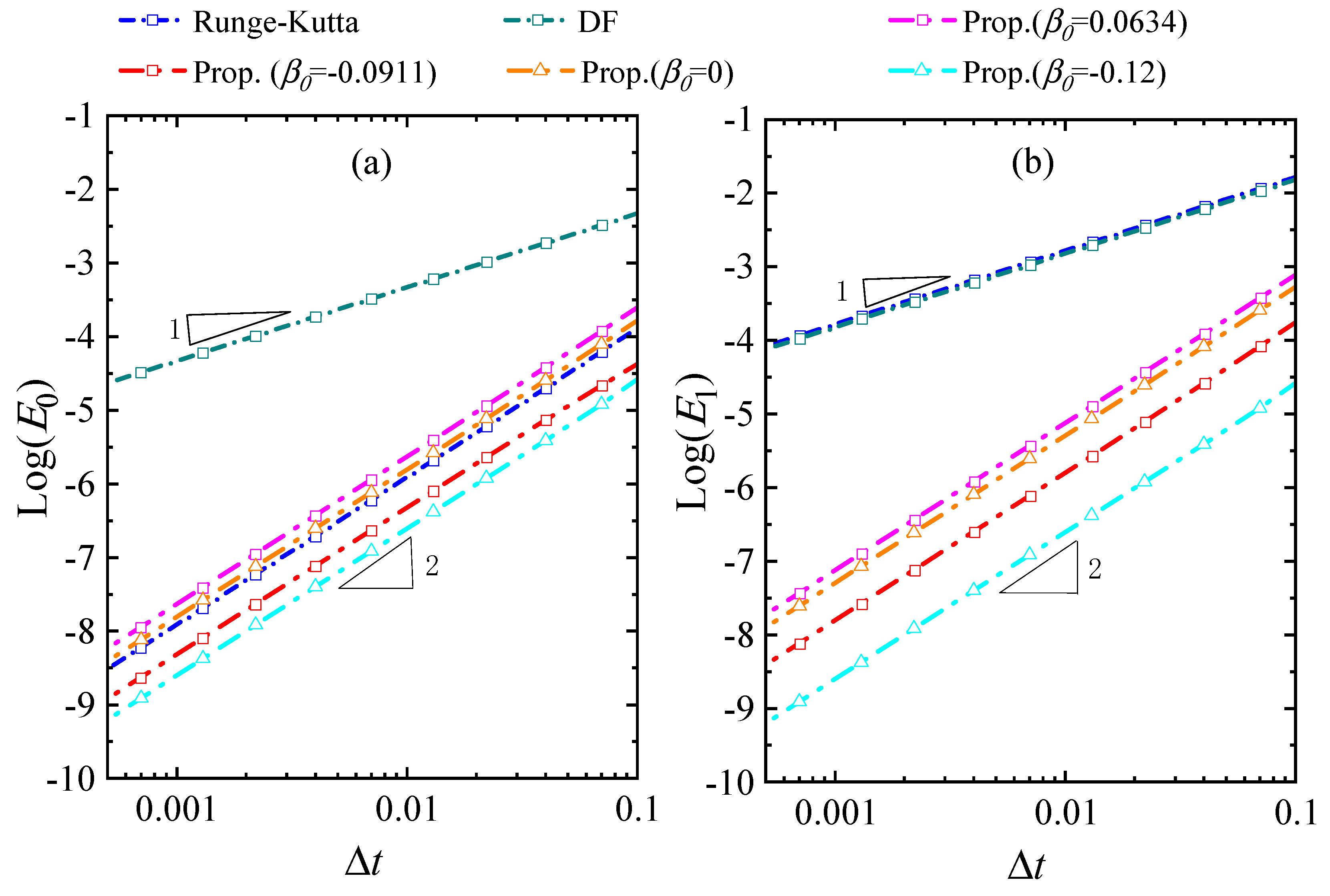
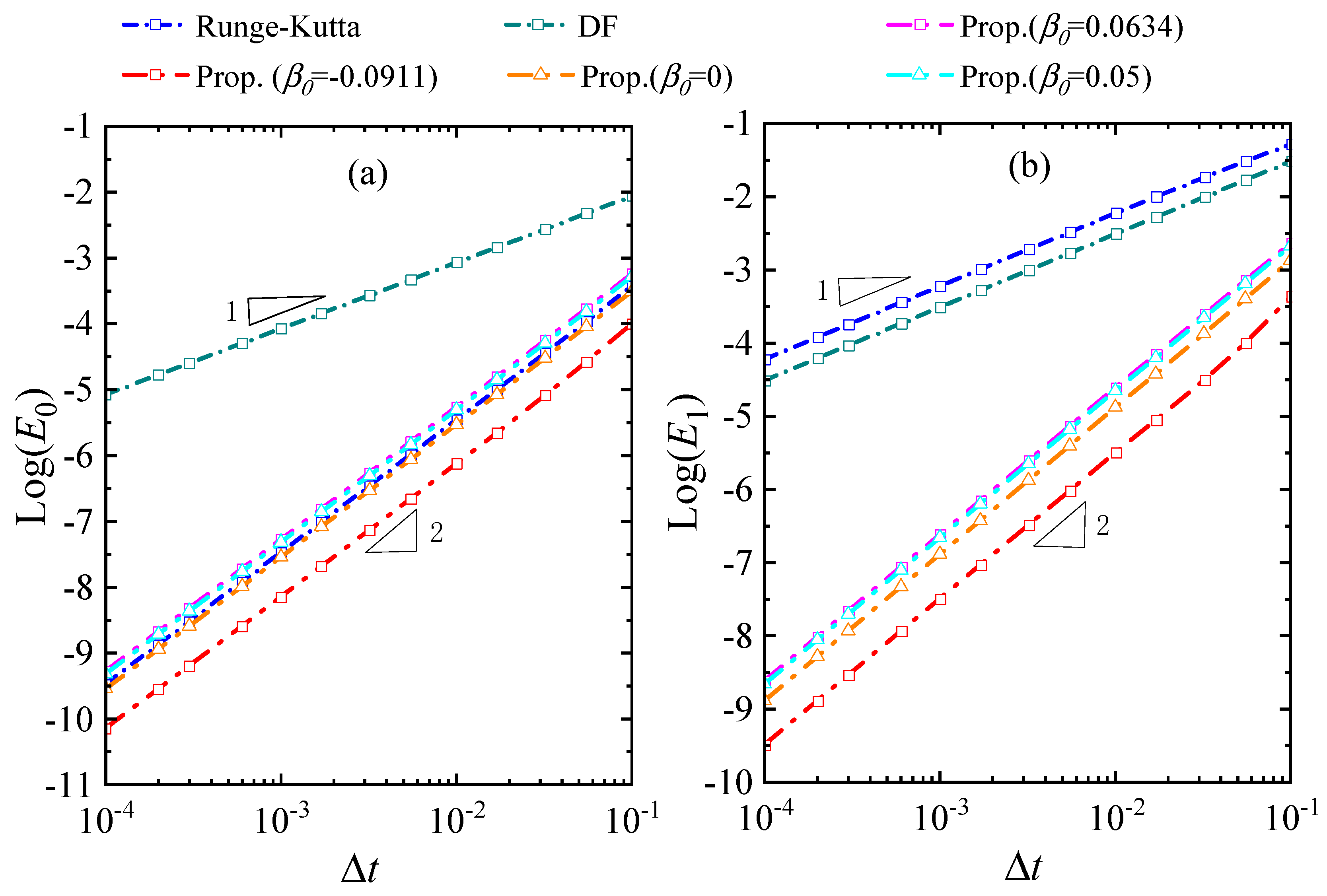
3.1. Accuracy Analysis

Consider an uncoupled single-degree-of-freedom (SDOF) system as follows:

$$\dot{T}+\omega T=q\left(t\right)$$

(23)

where $T$ is the temperature of the system. q is the external heat source. $\omega$ is thermal diffusivity, which is determined according to the actual system. The initial condition is given as follows:

$$T\left(t_i\right)=T_i$$

(24)

where $T_i$ is the initial temperature. Let $q\left(t\right)=q_0{e}^{{\omega }_{0}t}$, where $q_0$ and ${\omega }_0$ are the amplitude and frequency of the external source, respectively.

The exact solution for $t=t_{i+1}$ can be obtained as follows:

$$\left\{\begin{array}{c}\tilde{T}\left(t_{i+1}\right)\\ ∆t\cdot \dot{\tilde{T}}\left(t_{i+1}\right)\end{array}\right\}=\tilde{\mathit{A}}\left\{T\left(t_i\right)\right\}+\tilde{\mathit{R}}$$

(25)

where the superscript ‘∼’ represents the exact solution.

$$\tilde{\mathit{A}}=e^{-\omega ∆t}\left[\begin{array}{c}1\\ -\omega ∆t\end{array}\right]$$

(26)

$$\tilde{\mathit{R}}={\displaystyle \frac{q_0{e}^{-\omega ∆t}}{\omega +{\omega }_0}}\left[\begin{array}{c}{e}^{\omega ∆t+{\omega }_0∆t}-1\\ ∆t\cdot \left({\omega }_0{e}^{\omega ∆t+{\omega }_0∆t}+\omega \right)\end{array}\right]$$

(27)

For the proposed method, the numerical solution at $t=t_{i+1}$ is obtained as follows:

$$\left\{\begin{array}{c}\overline{T}\left(t_{i+1}\right)\\ ∆t\cdot \dot{\overline{T}}\left(t_{i+1}\right)\end{array}\right\}=\overline{\mathit{A}}\left\{T\left(t_i\right)\right\}+\overline{\mathit{R}}$$

(28)

where the superscript ‘-’ represents the numerical solution. The items of $\overline{\mathit{R}}$ are given in Appendix A. $\overline{\mathit{A}}$ is expressed as follows:

$$\overline{\mathit{A}}=\mathit{A}\left[\begin{array}{c}1\\ -\omega ∆t\end{array}\right]$$

(29)

where $\mathit{A}$ is the numerical amplification matrix. The items of $\mathit{A}$ are given in Appendix B.

With Taylor expansions, the differences between $\overline{\mathit{A}}$ and $\tilde{\mathit{A}}$ are obtained as follows:

$${\tilde{a}}_1-{\overline{a}}_1=\phi \left({\beta }_0\right){{\omega }^3\left(∆t\right)}^3+O\left({\left(∆t\right)}^4\right)$$

(30)

$${\tilde{a}}_2-{\overline{a}}_2={\displaystyle \frac{{\omega }^4}{6}}\cdot {\left(∆t\right)}^3+O\left({\left(∆t\right)}^4\right)$$

(31)

in which

$$\phi \left({\beta }_0\right)={\displaystyle \frac{3{\beta }_2\left(\mathrm{c}\mathrm{o}\mathrm{s}\left(\eta \right)-1\right)+\mathrm{s}in\left(\eta \right)}{6\left(\mathrm{c}\mathrm{o}\mathrm{s}\left(\eta \right)-1\right)}}$$

(32)

where ${\overline{a}}_k$ and ${\tilde{a}}_k$ represent the items of row $k$ in $\overline{\mathit{A}}$ and $\tilde{\mathit{A}}$, respectively.

Analogously, the differences between $\overline{\mathit{R}}$ and $\tilde{\mathit{R}}$ are obtained as follows:

$${\tilde{r}}_1-{\overline{r}}_1={\displaystyle \frac{q_0}{6}}\left(\left({\beta }_0-{\beta }_1-2{\beta }_2\right){{\omega }_0}^2+\left(3{\beta }_2-1\right)\left(\omega {\omega }_0-{\omega }^2\right)\right){\left(∆t\right)}^3+O\left({\left(∆t\right)}^4\right)$$

(33)

$${\tilde{r}}_2-{\overline{r}}_2={\displaystyle \frac{q_0{\omega }^2\left(\omega -{\omega }_0\right)}{6}}\cdot {\left(∆t\right)}^3+O\left({\left(∆t\right)}^4\right)$$

(34)

where ${\overline{r}}_k$ and ${\tilde{r}}_k$ represent the items of row $k$ in $\overline{\mathit{R}}$ and $\tilde{\mathit{R}}$, respectively. It can be observed that the proposed method can achieve at least second-order accuracy.

To obtain the third-order accuracy for the no external heat source case, it is required to satisfy $\phi \left({\beta }_0\right)=0$, which leads to the following:

$${\beta }_0={\displaystyle \frac{5\eta \mathrm{c}\mathrm{o}\mathrm{s}\left(\frac{\eta }{2}\right)-5\eta \mathrm{c}\mathrm{o}{\mathrm{s}}^3\left(\frac{\eta }{2}\right)-4{\eta }^2\mathrm{s}\mathrm{i}\mathrm{n}\left(\frac{\eta }{2}\right)-2\mathrm{s}\mathrm{i}{\mathrm{n}}^3\left(\frac{\eta }{2}\right)+{\eta }^3\mathrm{c}\mathrm{o}{\mathrm{s}}^3\left(\frac{\eta }{2}\right)+4{\eta }^2\mathrm{s}\mathrm{i}{\mathrm{n}}^3\left(\frac{\eta }{2}\right)}{3\eta \mathrm{c}\mathrm{o}\mathrm{s}\left(\frac{\eta }{2}\right)\left(1-\mathrm{c}\mathrm{o}{\mathrm{s}}^2\left(\frac{\eta }{2}\right)+{\eta }^2\mathrm{c}\mathrm{o}{\mathrm{s}}^2\left(\frac{\eta }{2}\right)-2\eta \mathrm{c}\mathrm{o}\mathrm{s}\left(\frac{\eta }{2}\right)\mathrm{s}\mathrm{i}\mathrm{n}\left(\frac{\eta }{2}\right)\right)}}$$

(35)

where for $\eta ={\displaystyle \frac{\pi }{2}}$, we have ${\beta }_0=-0.0911$.

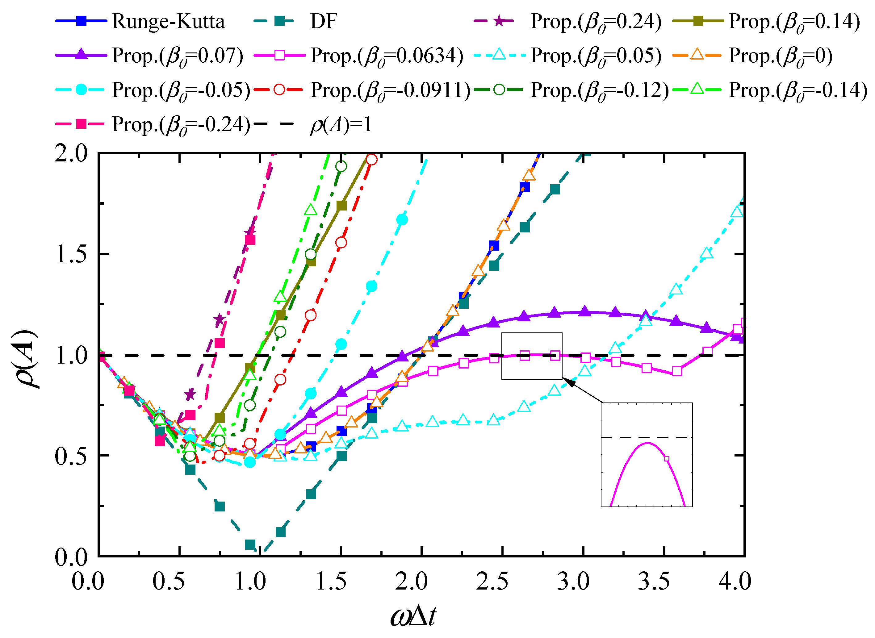
3.2. Spectral Stability

The characteristic polynomial of A is defined as follows:

$$P\left(\lambda \right)={\lambda }^2-2A_1\lambda +A_2$$

(36)

where the expressions of $A_1$ and $A_2$ are given in Appendix C. For the $\eta ={\displaystyle \frac{\pi }{2}}$ case, there are the following equations:

$$A_1=\left({\displaystyle \frac{{\beta }_2}{2}}+{\displaystyle \frac{1}{4}}\right){\left(\omega ∆t\right)}^2-\left({\displaystyle \frac{\pi {\beta }_1}{4}}+{\displaystyle \frac{{\beta }_2}{2}}+{\displaystyle \frac{1}{2}}\right)\left(\omega ∆t\right)+{\displaystyle \frac{1}{2}}$$

(37)

$$A_2=\left(-{\beta }_0+{\beta }_1-{\displaystyle \frac{\pi {\beta }_1}{4}}\right){\left(\omega ∆t\right)}^2+\left({\beta }_0-{\beta }_1\right)\left(\omega ∆t\right)$$

(38)

The spectral radius $\rho \left(\mathit{A}\right)$ is defined as follows:

$$\rho \left(\mathit{A}\right)=max\left(‖{\lambda }_1‖,‖{\lambda }_2‖\right)$$

(39)

where ${\lambda }_i\left(i=1, 2\right)$ are the roots of $P\left(\lambda \right)=0$, which are calculated using the following:

$${\lambda }_{\mathrm{1,2}}=\left(A_1\pm \sqrt{A_1^2-A_2}\right)$$

(40)

When $\rho \left(\mathit{A}\right)⩽1$, the proposed explicit method is stable. At the critical time step $∆t_c$, we have $\rho \left(\mathit{A}\left(∆t_c\right)\right)=1$.

Through mathematical solving, we found when ${\beta }_0=0.0634$, the maximal stable region for the proposed method is obtained. For comparison, the spectral radius curves from the DF method, the Runge–Kutta method (second-order), and the proposed method are plotted in Figure 1. It is found that the ${\beta }_0=0$ case shows an identical spectral radius as the Runge–Kutta method. Among all the considered methods, the ${\beta }_0=0.0634$ case of the proposed method displays a maximal stable region. For clarity, the $\omega ∆t_c$ values for various ${\beta }_0$ cases of the proposed method are provided in

Table 2. ωΔt_c for various parameter values of the proposed method.

β0	−0.24	−0.14	−0.12	−0.0911	−0.05	0	0.05	0.0634	0.07	0.14	0.24
ωΔtc	0.723	0.986	1.062	1.199	1.464	2	3.154	3.731	1.910	0.980	0.660

.

4. Illustrative Numerical Examples

In this section, some heat conduction examples are tested to evaluate the performance of the proposed method. These examples include two linear SDOF systems, a nonlinear SDOF system, a linear multi-degree-of-freedom (MDOF) system, a one-dimensional (1D) linear problem, a 1D nonlinear problem, two two-dimensional (2D) linear problem, and a three-dimensional (3D) linear problem. Some competitive methods, including the DF method and the second-order Runge–Kutta method [7], are also considered for comparison.

For the proposed method, the parameter cases are selected with the following consideration: (1) the ${\beta }_0=0.0634$ case with the maximal stable region; (2) ${\beta }_0=-0.0911$ case with third-order accuracy; (3) the ${\beta }_0=0$ case with the same spectral stability as the Runge–Kutta method; and (4) the other ${\beta }_0$ cases are exclusively selected according to the practical problems.

To characterize the accuracy of numerical results, we define the relative and global error norms as follows [29]:

$${\epsilon }_0=\left|{\displaystyle \frac{{\overline{T}}_i-{\tilde{T}}_i}{{\tilde{T}}_i}}\right|,{\epsilon }_1=\left|{\displaystyle \frac{{\dot{\overline{T}}}_i-{\dot{\tilde{T}}}_i}{{\dot{\tilde{T}}}_i}}\right|$$

(41)

and

$$E_0=\sqrt{{\displaystyle \frac{\sum _{i=1}^{NT}{\left({\overline{T}}_i-{\tilde{T}}_i\right)}^2}{\sum _{i=1}^{NT}{\left({\tilde{T}}_i\right)}^2}}},E_1=\sqrt{{\displaystyle \frac{\sum _{i=1}^{NT}{\left({\dot{\overline{T}}}_i-{\dot{\tilde{T}}}_i\right)}^2}{\sum _{i=1}^{NT}{\left({\dot{\tilde{T}}}_i\right)}^2}}}$$

(42)

where ${\overline{T}}_i$ and ${\tilde{T}}_i$ represent the numerical and exact solutions of temperature at time $t_i$, respectively. ${\dot{\overline{T}}}_i$ and ${\dot{\tilde{T}}}_i$ represent the numerical and exact solutions of temperature derivative, respectively. NT is the total number of discrete times. For complex problems, exact or analytical solutions are difficult to obtain, so a quasi-exact solution for reference is obtained using the Crank–Nicolson method [8] with very small time step.

4.1. A Linear SDOF System with Simple External Heat Source

In this section, a linear SDOF system is considered for the test [34].

$$\dot{T}+\omega T=F\left(t\right),T_0=15,\omega =1$$

(43)

Firstly, $F\left(t\right)=20\mathrm{c}\mathrm{o}\mathrm{s}\left(0.3t\right)$ is considered, and the exact solution of Equation (43) can be given as follows:

$$T\left(t\right)=\left(T_0-{\displaystyle \frac{2000\omega }{9+100{\omega }^2}}\right)e^{-\omega t}+{\displaystyle \frac{200\left[10\omega cos\left(0.3t\right)+3sin\left(0.3t\right)\right]}{9+100{\omega }^2}}$$

(44)

A time history of 0–40 s is considered. Figure 2 shows the global errors from all the considered methods.

It is observed that the DF method achieves first-order accuracy. The Runge–Kutta method achieves second-order accuracy for temperature and first-order accuracy for the temperature derivative. The proposed methods provide second-order accuracy for all the physical variables. It is worth noting that the proposed method ${(\beta }_0=-0.12$) can provide the highest calculation accuracy among all the considered methods. It can be seen that the Runge–Kutta method has a similar accuracy as the proposed method ${(\beta }_0=0$) for temperature. However, for temperature derivative, the accuracy of the proposed method ${(\beta }_0=0$) is much higher than that of the Runge–Kutta method.

Then, a parabolic heat source $F\left(t\right)=-t^2+10t$ is adopted, and the exact solution of Equation (43) is as follows:

$$T\left(t\right)=\left(T_0+{\displaystyle \frac{10\omega +2}{{\omega }^3}}\right)e^{-\omega t}-{\displaystyle \frac{t^2}{{\omega }^2}}+{\displaystyle \frac{\left(10\omega +2\right)\left(\omega t-1\right)}{{\omega }^3}}$$

(45)

Figure 3 shows the global errors from all the considered methods. It is observed that the proposed method also exhibits higher accuracy than the other methods. Moreover, the ${\beta }_0=-0.0911$ case of the proposed method can achieve the highest accuracy.

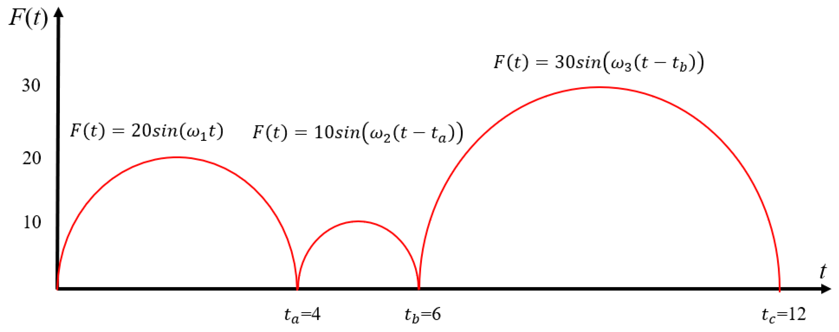
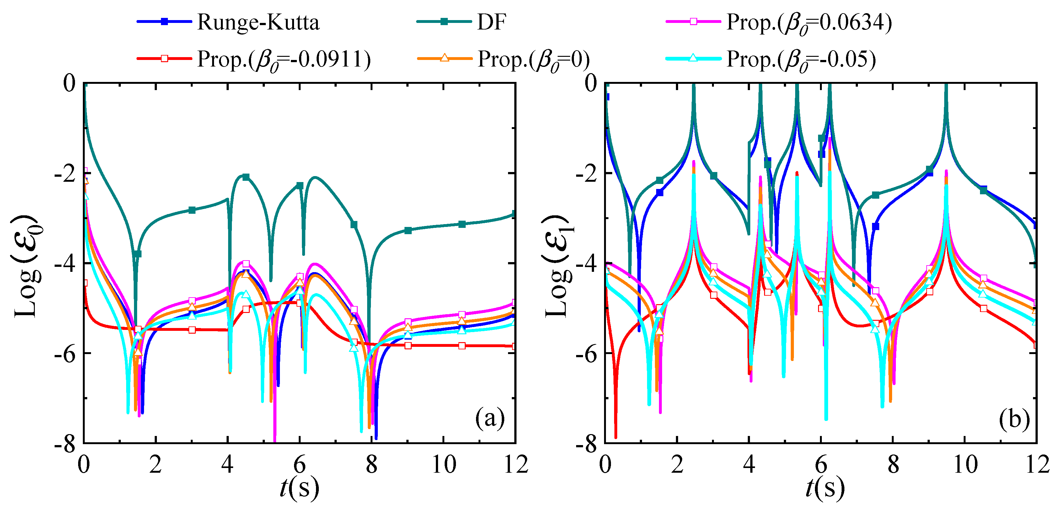
4.2. A Linear SDOF System with Complex External Heat Source

Here, we consider an SDOF system with an external heat source described by piecewise trigonometric functions [29]. The governing equation can be written as follows:

$$\dot{T}+\omega T=F\left(t\right),T_0=0$$

(46)

where $\omega =2$, and $F\left(t\right)$ is given as follows:

$$F\left(t\right)=\left\{\begin{array}{c}20sin\left({\omega }_{1}t\right), 0<t\le t_a\\ 10sin\left({\omega }_2\left(t-t_a\right)\right),t_a<t\le t_b\\ 30sin\left({\omega }_3\left(t-t_b\right)\right),t_b<t\le t_c\end{array}\right.$$

(47)

where ${\omega }_1={\displaystyle \frac{\pi }{2}}$, ${\omega }_2={\displaystyle \frac{\pi }{4}}$, ${\omega }_3={\displaystyle \frac{\pi }{6}}$. $F\left(t\right)$ is plotted in Figure 4.

The exact solution for this problem is obtained as follows:

$$T\left(t\right)=\left\{\begin{array}{c}20\left({\displaystyle \frac{\omega sin\left({\omega }_{1}t\right)-{\omega }_{1}cos\left({\omega }_{1}t\right)}{{{\omega }_1}^2+{\omega }^2}}+{\displaystyle \frac{{\omega }_1}{{{\omega }_1}^2+{\omega }^2}}\cdot e^{-\omega t}\right), 0<t\le t_a\\ 10\left({\displaystyle \frac{\omega sin\left({\omega }_2\left(t-t_a\right)\right)-{\omega }_{2}cos\left({\omega }_2\left(t-t_a\right)\right)}{{{\omega }_2}^2+{k\omega }^2}}+\left({\displaystyle \frac{T_a}{10}}+{\displaystyle \frac{{\omega }_2}{{{\omega }_2}^2+{\omega }^2}}\right)\cdot e^{-\omega \left(t-t_a\right)}\right),t_a<t\le t_b\\ 30\left({\displaystyle \frac{\omega sin\left({\omega }_3\left(t-t_b\right)\right)-{\omega }_{3}cos\left({\omega }_3\left(t-t_b\right)\right)}{{{\omega }_3}^2+{\omega }^2}}+\left({\displaystyle \frac{T_b}{30}}+{\displaystyle \frac{{\omega }_3}{{{\omega }_3}^2+{\omega }^2}}\right)\cdot e^{-\omega \left(t-t_b\right)}\right),t_b<t\le t_c\end{array}\right.$$

(48)

where

$$T_a=20\left({\displaystyle \frac{\omega sin\left({\omega }_1{t}_a\right)-{\omega }_1\mathrm{c}\mathrm{o}\mathrm{s}\left({\omega }_1{t}_a\right)}{{{\omega }_1}^2+{\omega }^2}}+{\displaystyle \frac{{\omega }_1}{{{\omega }_1}^2+{\omega }^2}}\cdot e^{-\omega t_a}\right)$$

(49)

$$T_b=10\left({\displaystyle \frac{\omega sin\left({\omega }_2\left(t_b-t_a\right)\right)-{\omega }_2\mathrm{c}\mathrm{o}\mathrm{s}\left({\omega }_2\left(t_b-t_a\right)\right)}{{{\omega }_2}^2+{\omega }^2}}+\left({\displaystyle \frac{T_a}{10}}+{\displaystyle \frac{{\omega }_2}{{{\omega }_2}^2+{\omega }^2}}\right)\cdot e^{-\omega \left(t_b-t_a\right)}\right)$$

(50)

The time step size Δt = 1 × 10⁻² s is selected. Figure 5 displays the log-form relative errors from the various methods. It is illustrated that among all the considered methods, the proposed method achieves the highest accuracy for both temperature and the temperature derivative, which demonstrates effectiveness of the proposed method for complex heat source problems.

4.3. A Nonlinear SDOF System

Here, a nonlinear radiation system is considered. The governing equation can be described by [34,35] the following:

$$\dot{T}+\sigma ϵ\left(T^4-T_{\mathrm{\infty }}^4\right)=0$$

(51)

where σ is a Stefan–Boltzmann constant, and ϵ is the emissivity of the surface. $T_{\mathrm{\infty }}$ is the ambient temperature which is chosen as $T_{\mathrm{\infty }}=0$. Then, the exact solution of Equation (51) can be obtained as follows:

$$T\left(t\right)={\displaystyle \frac{T_0}{{\left(3\sigma ϵT_0^{3}t+1\right)}^{1/3}}}$$

(52)

where $\sigma =5.6703e^{-8},ϵ=0.5$, and $T_0=250$. Here, the time history of 0.0–10.0 s is tested.

In Figure 6, the global error results from all the methods are plotted. Similar to the solution of the linear SDOF system, the DF method provides first-order accuracy for all the physical variables. The Runge–Kutta method only provides second-order accuracy for temperature. The proposed methods achieve second-order accuracy for temperature and its derivative. It is observed that the proposed method ${(\beta }_0=-0.0911)$ can achieve the highest accuracy.

4.4. A Linear MDOF System

A two-DOF (two nodes) system with no external heat source is considered. The time history for test is 0.0–5.0 s. The basic parameters of the system are $K=\left[\begin{array}{cc}-998& -1998\\ 999& 1999\end{array}\right]$. The governing equation is given as follows [36]:

$$\left[\begin{array}{c}{\dot{T}}_1\\ {\dot{T}}_2\end{array}\right]+K\left[\begin{array}{c}{T}_1\\ T_2\end{array}\right]=0$$

(53)

The initial temperature is $\left[\begin{array}{c}{T}_1\\ T_2\end{array}\right]=\left[\begin{array}{c}1\\ 0\end{array}\right]$, the analytical solution of Equation (53) can be obtained as follows:

$$\left[\begin{array}{c}{T}_1\\ T_2\end{array}\right]=\left[\begin{array}{c}2e^{-t}-e^{-1000t}\\ -e^{-t}+e^{-1000t}\end{array}\right]$$

(54)

In Figure 7 and Figure 8, the global error results of all the methods are illustrated. It can be observed that the proposed method ${(\beta }_0=-0.0911$) has third-order accuracy, which is much higher than those of the other methods. This is consistent with the accuracy analysis in Section 3.1.

For fair comparison, in

Table 3. The computational time cost of the various methods for different time steps.

Δt	Runge–Kutta	DF	Prop.
			β0 = 0.0634	β0 = −0.0911	β0 = 0	β0 = 0.05
0.001	0.02819	0.01735	0.06422	0.06313	0.06437	0.06566
0.0005	0.05590	0.03203	0.12570	0.12448	0.12256	0.12639
0.0001	0.25360	0.14495	0.59931	0.60162	0.59537	0.59457

, the time costs of the various methods under the same $\mathsf{\Delta }t$ are shown to illustrate computation efficiency of the proposed method. It is observed that all the methods have small computational costs. The proposed method achieves a notable accuracy improvement with minimal efficiency loss.

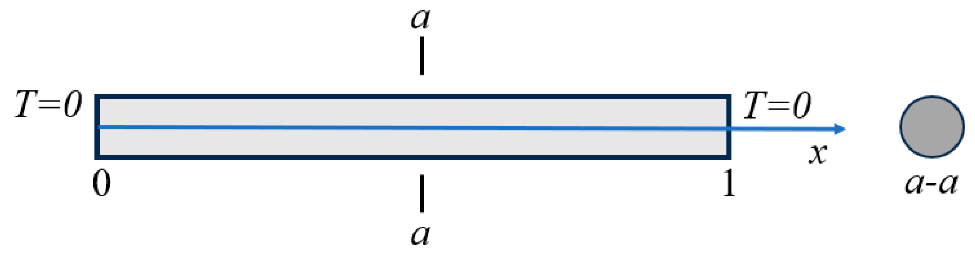
4.5. A Linear 1D System

In this example, we analyze a uniform 1D bar over a time history from 0.0 s to 1.0 s. The bar, as shown in Figure 9, has length L = 1, with both ends maintained at a fixed temperature of 0 K. The governing equation for this problem can be written as follows:

$${\displaystyle \frac{\partial T}{\partial t}}={\displaystyle \frac{{\partial }^{2}T}{\partial x^2}}$$

(55)

The initial temperature distribution within the bar is given by the following [36,37]:

$$T\left(x,0\right)=sin\left(\pi x\right),0<x<L$$

(56)

The exact solution can be obtained as follows:

$$T\left(x,t\right)=\mathrm{s}\mathrm{i}\mathrm{n}\left(\pi x\right)e^{-{\pi }^{2}t}$$

(57)

The bar is discretized by 40 two-node bar elements. The same time step size Δt = 5 × 10⁻⁵ s is selected for all the considered methods to satisfy stability.

Figure 10 shows the relative error results at point $x=0.5$. It is observed that the ${\beta }_0=-0.0911$ case achieves a similar accuracy as the DF method, and the ${\beta }_0=0$ case achieves a similar accuracy as the Runge–Kutta method. It is noteworthy that the ${\beta }_0=0.14$ case can give the highest accuracy. Figure 11 displays the relative errors for temperature and its derivative along the entire rod at t = 0.5 s. The curves show that the proposed method maintains good accuracy for both temperature and its derivative throughout the bar. Especially, the ${\beta }_0=0.14$ case exhibits the highest solution accuracy.

4.6. A Nonlinear 1D System

Here, a nonlinear 1D bar with temperature-dependent material parameters is considered. The time history of 0.0–0.5 s is tested. The geometric size and boundary conditions of the bar are same as those of the linear 1D bar, as shown in Figure 9. The governing equation can be written as follows [35,38]:

$${\displaystyle \frac{\partial T}{\partial t}}={\displaystyle \frac{\partial }{\partial x}}\left(\left(1+T\right){\displaystyle \frac{\partial T}{\partial x}}\right)$$

(58)

The initial conditions are given as follows:

$$T\left(x,0\right)=1$$

(59)

In analysis, 20 two-node bar elements are employed for spatial discretization, and time step size Δt = 1 × 10⁻⁴ s is selected for all the methods.

In Figure 12, the relative errors of temperature and its derivative at $x=0.5$ are plotted. It is observed that the proposed method can provide more accurate solutions than those of the other methods. Especially, the ${\beta }_0=0.05$ case exhibits the highest accuracy for temperature and its derivative.

4.7. A 2D Square Plate

Consider a homogeneous square plate, as shown in Figure 13. The boundaries at $x=0$ and $y=1$ are insulated, and the side boundary at $x=1$ undergoes convection with a heat flux q(t) = cos(10t) [35,39]. The bottom boundary maintains a temperature field of $T=0$. The governing equation and the initial conditions are as follows:

$${\displaystyle \frac{\partial T}{\partial t}}={\displaystyle \frac{{\partial }^{2}T}{\partial x^2}}+{\displaystyle \frac{{\partial }^{2}T}{\partial y^2}},T\left(x,y,0\right)=0$$

(60)

The model is discretized by 100 four-node finite elements. A time step size Δt = 3 × 10⁻⁴ s and a time duration of 0.0–1.5 s is considered.

Figure 14 and Figure 15 illustrate the relative errors of temperature and its derivative at the point $\left(x,y\right)=\left(0.5, 0.5\right)$, respectively. It is observed that the proposed method ${(\beta }_0=-0.24)$ demonstrates higher accuracy than those of the other methods.

4.8. A 2D Air Fin Heat Dissipation Structure

Figure 16 shows a rectangular air fin heat dissipation structure (0.09 m × 0.06 m), which is frequently used in electronic chip cooling systems [40]. The geometric dimensions and boundary conditions of the structure are also illustrated, and the structure is discretized with 272 three-node triangular elements. The bottom boundary is prescribed with periodic heat flux density $q\left(t\right)=50\sin \left(t\right)+10$ kW. All the other faces experience heat convection, with a convection heat transfer coefficient h = 200 W/m²·K and an ambient temperature T_∞ = 0 K. The initial temperature for all the nodes is T₀ = 37 K. The material properties are given as follows: isotropic thermal conductivity ω = 120 W/m·K, density ρ = 3000 kg/m³, and specific heat capacity c = 1000 J/kg·K. The governing equation is given as follows:

$$\rho c{\displaystyle \frac{\partial T}{\partial t}}=\omega \left({\displaystyle \frac{{\partial }^{2}T}{\partial x^2}}+{\displaystyle \frac{{\partial }^{2}T}{\partial y^2}}\right)$$

(61)

A time step size Δt = 1 × 10⁻² s and a time duration of 0.0–30.0 s are considered. In Figure 17, the relative errors from the various methods at node A are presented. It is observed that the proposed method ${(\beta }_0=0)$ exhibits the highest accuracy for temperature, and the proposed method ${(\beta }_0=-0.0911)$ demonstrates a higher accuracy than those of the other methods for the temperature derivative.

Figure 18 illustrates the relative errors at node B. It is observed that the ${\beta }_0=-0.0911$ case of the proposed method exhibits the highest accuracy for temperature, and the ${\beta }_0=-0.14$ case provides highest accurate solutions for the temperature derivative.

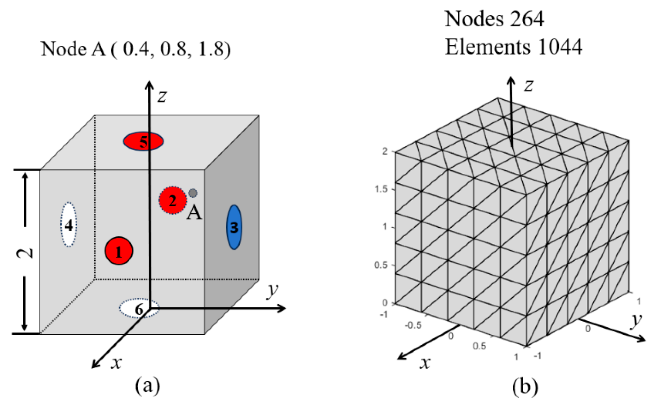
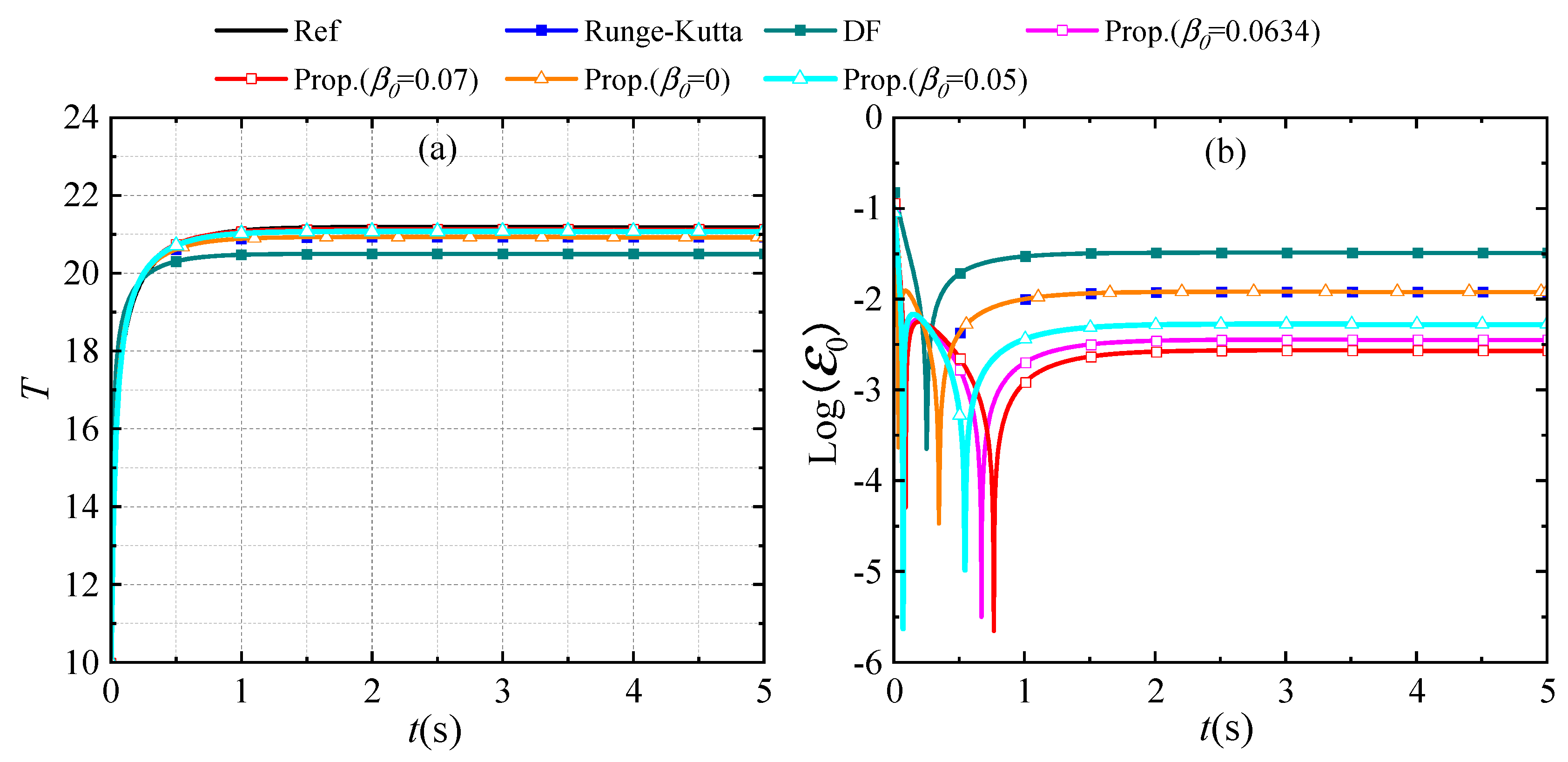
4.9. A 3D Cube Model

Here, a 3D cube model, as shown in Figure 19, is considered for the heat conduction test [41]. The dimensionless geometric configuration is shown in this figure. The governing equation and the initial conditions are given as follows:

$${\displaystyle \frac{\partial T}{\partial t}}={\displaystyle \frac{{\partial }^{2}T}{\partial x^2}}+{\displaystyle \frac{{\partial }^{2}T}{\partial y^2}}+{\displaystyle \frac{{\partial }^{2}T}{\partial z^2}},T\left(x,y,z,0\right)=10$$

(62)

A fixed temperature T = 20 is imposed on surfaces 1, 2, and 5. The heat flux density q_n = −50 acts on surface 3. The adiabatic boundary acts on surfaces 4 and 6. As shown in Figure 19b, the structure is discretized with 1044 four-node tetrahedral finite elements. The internal node A is considered for the test. Δt = 5 × 10⁻³ s and a time duration of 0.0–5.0s are selected.

In Figure 20a, the temperatures from the various methods at node A are presented. It is observed that the calculation results of the DF method obviously deviate from the reference solution, while the other methods have little deviation. In Figure 20b, relative error curves of temperature are illustrated. It is observed that the proposed method demonstrates slightly higher temperature accuracy than those of the other methods. The proposed method ${(\beta }_0=0.07)$ exhibits the highest accuracy for temperature.

5. Conclusions

This study introduces a new explicit time integration scheme based on uniform trigonometric B-spline interpolation for transient heat conduction problems. The proposed method exhibits a desirable performance in both accuracy and stability. Through the numerical experiments and theoretical analysis, the following conclusions can be drawn.

(1)

The proposed method has one free parameter (${\beta }_0$) that can be used to control the basic algorithmic properties. With specific parameters, the proposed method demonstrates superior stability compared to those of the traditional methods.

(2)

Through numerical analyses, we recommend the ${\beta }_0=0.0634$ case of the proposed method for large-scale systems. It allows for a large time step and can trade-off efficiency and accuracy. For uncoupled multi-degree-of-freedom problems, especially those without heat sources, the 0.0911 case is suggested, as it can significantly enhance accuracy.

(3)

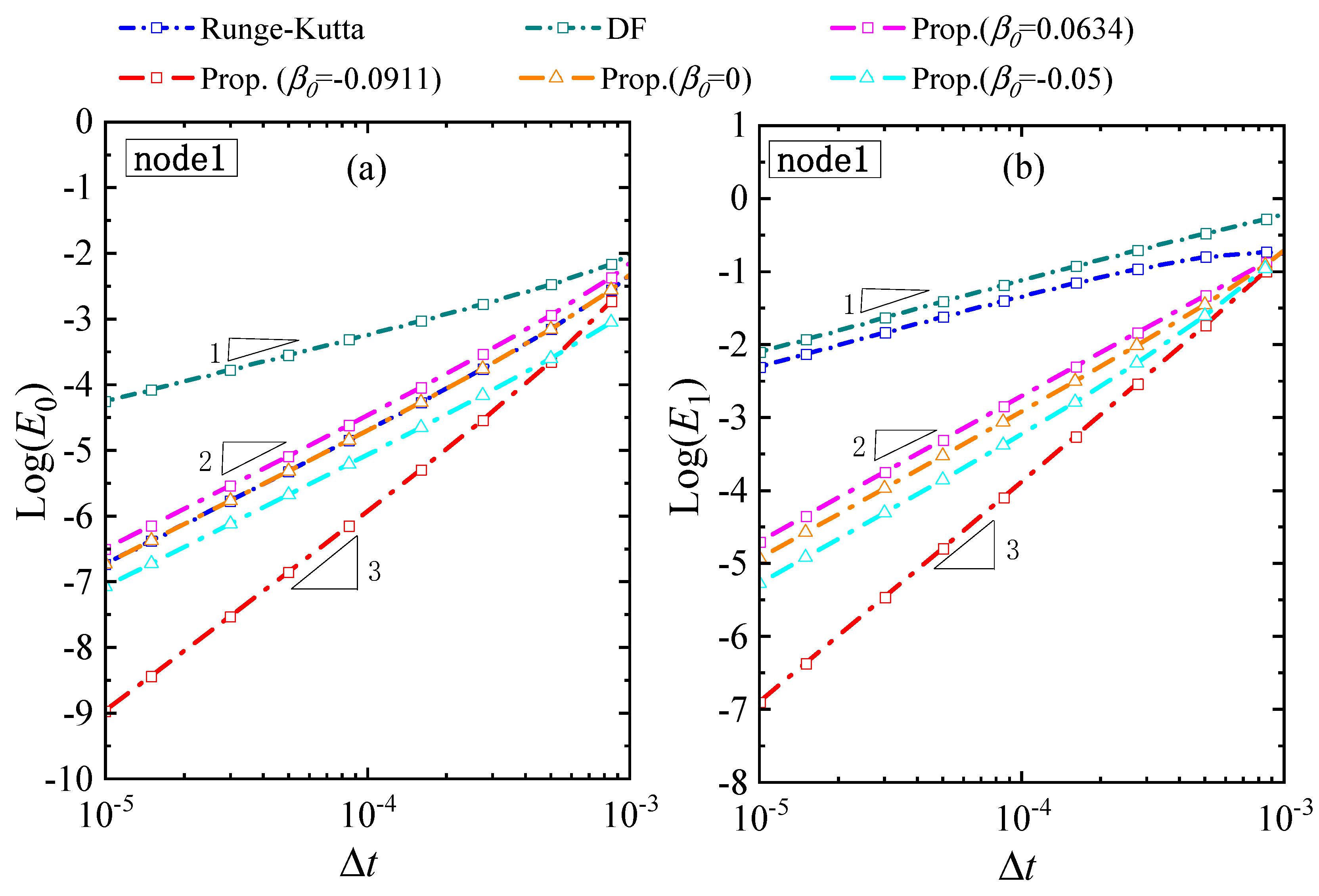
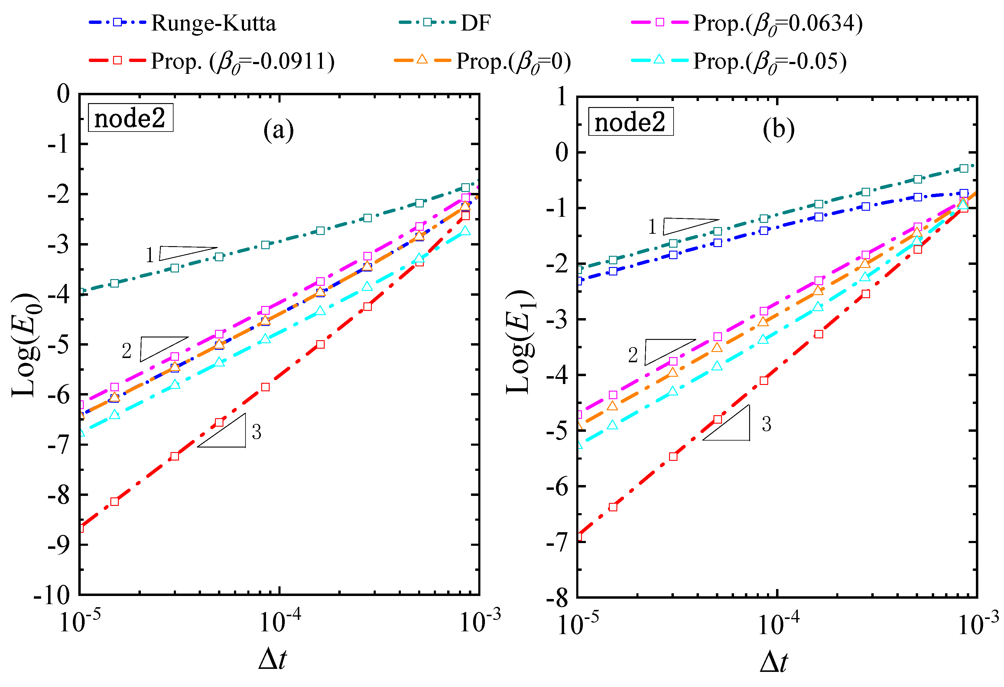
Through theoretical analysis, the proposed method achieves at least second-order accuracy for temperature and its derivative. In some special cases, it can reach third-order accuracy for temperature.

(4)

For linear systems, the proposed method achieves desirable accuracy. As for nonlinear systems, the proposed method is effective and provides desirable solution accuracy.

(5)

In the proposed method, the integral weak form of the heat conduction equations is introduced to capture the variation in external heat source, which intrinsically improves the computation accuracy.

(6)

In future research, the proposed method may be integrated with other high-order spatial elements (numerical manifold elements [42], quasi-smooth manifold elements [43], etc.) to further improve the solution accuracy for complex transient heat conduction problems.

References

1. Lei, J.; Wang, Q.; Liu, X.; Gu, Y.; Fan, C.-M. A Novel Space-Time Generalized FDM for Transient Heat Conduction Problems. Eng. Anal. Bound. Elem. 2020, 119, 1–12. [Google Scholar] [CrossRef]
2. Kubacka, E.; Ostrowski, P. Heat Conduction Issue in Biperiodic Composite Using Finite Difference Method. Compos. Struct. 2021, 261, 113310. [Google Scholar] [CrossRef]
3. Zhang, J.; Chauhan, S. Fast Explicit Dynamics Finite Element Algorithm for Transient Heat Transfer. Int. J. Therm. Sci. 2019, 139, 160–175. [Google Scholar] [CrossRef]
4. Suvin, V.; Ooi, E.T.; Song, C.; Natarajan, S. Temperature-Dependent Nonlinear Transient Heat Conduction Using the Scaled Boundary Finite Element Method. Int. J. Heat Mass Transf. 2025, 243, 126780. [Google Scholar] [CrossRef]
5. Meng, Z.; Ma, Y.; Ma, L. A Fast Interpolating Meshless Method for 3D Heat Conduction Equations. Eng. Anal. Bound. Elem. 2022, 145, 352–362. [Google Scholar] [CrossRef]
6. Noh, G.; Bathe, K.-J. An Explicit Time Integration Scheme for the Analysis of Wave Propagations. Comput. Struct. 2013, 129, 178–193. [Google Scholar] [CrossRef]
7. Time Discretization of Equations of Motion: Overview and Conventional Practices. In Advances in Computational Dynamics of Particles, Materials and Structures; John Wiley & Sons, Ltd.: Hoboken, NJ, USA, 2012; pp. 493–552. ISBN 978-1-119-96589-3.
8. Crank, J.; Nicolson, P. A Practical Method for Numerical Evaluation of Solutions of Partial Differential Equations of the Heat-Conduction Type. Math. Proc. Camb. Phil. Soc. 1947, 43, 50–67. [Google Scholar] [CrossRef]
9. Newmark, N.M. A Method of Computation for Structural Dynamics. J. Eng. Mech. Div. 1959, 85, 67–94. [Google Scholar] [CrossRef]
10. Chung, J.; Hulbert, G.M. A Time Integration Algorithm for Structural Dynamics with Improved Numerical Dissipation: The Generalized-α Method. J. Appl. Mech. 1993, 60, 371–375. [Google Scholar] [CrossRef]
11. Zhang, J.; Liu, Y.; Liu, D. Accuracy of a Composite Implicit Time Integration Scheme for Structural Dynamics. Int. J. Numer. Methods Eng. 2017, 109, 368–406. [Google Scholar] [CrossRef]
12. Wen, W.; Wu, L.; Liu, T.; Deng, S.; Duan, S. A Novel Three Sub-Step Explicit Time Integration Method for Wave Propagation and Dynamic Problems. Int. J. Numer. Methods Eng. 2023, 124, 3299–3328. [Google Scholar] [CrossRef]
13. Liu, T.; Wang, P.; Wen, W. An Improved Time-Marching Formulation Based on an Explicit Time Integration Method for Dynamic Analysis of Non-Viscous Damping Systems. Mech. Syst. Signal Process. 2023, 191, 110195. [Google Scholar] [CrossRef]
14. Zhai, W.-M. Two Simple Fast Integration Methods for Large-Scale Dynamic Problems in Engineering. Int. J. Numer. Meth. Engng. 1996, 39, 4199–4214. [Google Scholar] [CrossRef]
15. Hulbert, G.M.; Chung, J. Explicit Time Integration Algorithms for Structural Dynamics with Optimal Numerical Dissipation. Comput. Methods Appl. Mech. Eng. 1996, 137, 175–188. [Google Scholar] [CrossRef]
16. Tchamwa, B.; Conway, T.; Wielgosz, C. An Accurate Explicit Direct Time Integration Method for Computational Structural Dynamics. In Proceedings of the Recent Advances in Solids and Structures, Nashville, TN, USA, 14 November 1999; American Society of Mechanical Engineers: Fairfield, NJ, USA, 1999; pp. 77–84. [Google Scholar]
17. Soares, D. A Novel Time-Marching Formulation for Wave Propagation Analysis: The Adaptive Hybrid Explicit Method. Comput. Methods Appl. Mech. Eng. 2020, 366, 113095. [Google Scholar] [CrossRef]
18. Malakiyeh, M.M.; Shojaee, S.; Hamzehei-Javaran, S.; Bathe, K.-J. The Explicit Β1/Β2-Bathe Time Integration Method. Comput. Struct. 2023, 286, 107092. [Google Scholar] [CrossRef]
19. Kim, W.; Reddy, J.N. Novel Explicit Time Integration Schemes for Efficient Transient Analyses of Structural Problems. Int. J. Mech. Sci. 2020, 172, 105429. [Google Scholar] [CrossRef]
20. Li, J.; Yu, K.; Zhao, R. Two Third-Order Explicit Integration Algorithms with Controllable Numerical Dissipation for Second-Order Nonlinear Dynamics. Comput. Methods Appl. Mech. Eng. 2022, 395, 114945. [Google Scholar] [CrossRef]
21. Liu, T.; Huang, F.; Wen, W.; Deng, S.; Duan, S.; Fang, D. An Improved Higher-Order Explicit Time Integration Method with Momentum Corrector for Linear and Nonlinear Dynamics. Appl. Math. Model. 2021, 98, 287–308. [Google Scholar] [CrossRef]
22. Wen, W.; Deng, S.; Duan, S.; Fang, D. A High-order Accurate Explicit Time Integration Method Based on Cubic B-spline Interpolation and Weighted Residual Technique for Structural Dynamics. Numer. Meth Eng. 2021, 122, 431–454. [Google Scholar] [CrossRef]
23. Liu, T.; Wang, P.; Wen, W.; Feng, F. Improved Explicit Quartic B-Spline Time Integration Scheme for Dynamic Response Analysis of Viscoelastic Systems. Mech. Syst. Signal Process. 2024, 208, 110982. [Google Scholar] [CrossRef]
24. Han, Y.; Liu, T.; Wen, W.; Liu, X. A New Family of B-Spline Based Explicit Time Integration Methods for Linear Structural Dynamic Analysis. Comput. Math. Appl. 2025, 185, 29–51. [Google Scholar] [CrossRef]
25. Liu, T.; Wang, P.; Wen, W.; Feng, F. Formulation and Analysis of a Cubic B-Spline-Based Time Integration Procedure for Structural Seismic Response Analysis. Int. J. Struct. Stab. Dyn. 2023, 23, 2350180. [Google Scholar] [CrossRef]
26. Zhang, Y.; Cao, J.; Chen, Z.; Li, X.; Zeng, X.-M. B-Spline Surface Fitting with Knot Position Optimization. Comput. Graph. 2016, 58, 73–83. [Google Scholar] [CrossRef]
27. Park, H. B-Spline Surface Fitting Based on Adaptive Knot Placement Using Dominant Columns. Comput.-Aided Des. 2011, 43, 258–264. [Google Scholar] [CrossRef]
28. Wen, W.-B.; Jian, K.-L.; Luo, S.-M. An Explicit Time Integration Method for Structural Dynamics Using Septuple B-Spline Functions. Int. J. Numer. Methods Eng. 2014, 97, 629–657. [Google Scholar] [CrossRef]
29. Wen, W.; Li, H.; Liu, T.; Deng, S.; Duan, S. A Novel Hybrid Sub-Step Explicit Time Integration Method with Cubic B-Spline Interpolation and Momentum Corrector Technique for Linear and Nonlinear Dynamics. Nonlinear Dyn. 2022, 110, 2685–2714. [Google Scholar] [CrossRef]
30. Nikolis, A. Numerical Solutions of Ordinary Differential Equations with Quadratic Trigonometric Splines. Appl. Math. E-Notes 2004, 4, 142–149. [Google Scholar]
31. Liu, T.; Wang, P.; Wen, W. A Novel Single-Step Explicit Time Integration Method Based on Momentum Corrector Technique for Structural Dynamic Analysis. Appl. Math. Model. 2023, 124, 1–23. [Google Scholar] [CrossRef]
32. Hughes, T.J.R. The Finite Element Method: Linear Static and Dynamic Finite Element Analysis; Dover Publications: Mineola, NY, USA, 2000; ISBN 978-0-486-13502-1. [Google Scholar]
33. Lü, Y.; Wang, G.; Yang, X. Uniform Trigonometric Polynomial B-Spline Curves. Sci. China Ser. F 2002, 45, 335–343. [Google Scholar] [CrossRef]
34. Wang, Y.; Maxam, D.; Tamma, K.K.; Qin, G. Design/Analysis of GEGS4-1 Time Integration Framework with Improved Stability and Solution Accuracy for First-Order Transient Systems. J. Comput. Phys. 2020, 422, 109763. [Google Scholar] [CrossRef]
35. Ji, Y.; Xing, Y. An Unconditionally Stable Method for Transient Heat Conduction. Lixue Xuebao/Chin. J. Theor. Appl. Mech. 2021, 53, 1951–1961. [Google Scholar] [CrossRef]
36. Song, Z.; Lai, S.-K.; Wu, B. A New MIB-Based Time Integration Method for Transient Heat Conduction Analysis of Discrete and Continuous Systems. Int. J. Heat Mass Transf. 2024, 222, 125153. [Google Scholar] [CrossRef]
37. Young, D.L.; Tsai, C.C.; Murugesan, K.; Fan, C.M.; Chen, C.W. Time-Dependent Fundamental Solutions for Homogeneous Diffusion Problems. Eng. Anal. Bound. Elem. 2004, 28, 1463–1473. [Google Scholar] [CrossRef]
38. Chen, B.; Gu, Y.; Guan, Z.; Zhang, H. Nonlinear Transient Heat Conduction Analysis with Precise Time Integration Method. Numer. Heat Transf. Part B Fundam. 2001, 40, 325–341. [Google Scholar] [CrossRef]
39. Li, Q.-H.; Chen, S.-S.; Kou, G.-X. Transient Heat Conduction Analysis Using the MLPG Method and Modified Precise Time Step Integration Method. J. Comput. Phys. 2011, 230, 2736–2750. [Google Scholar] [CrossRef]
40. Yang, K.; Jiang, G.-H.; Li, H.-Y.; Zhang, Z.; Gao, X.-W. Element Differential Method for Solving Transient Heat Conduction Problems. Int. J. Heat Mass Transf. 2018, 127, 1189–1197. [Google Scholar] [CrossRef]
41. Sun, W.; Qu, W.; Gu, Y.; Li, P.-W. An Arbitrary Order Numerical Framework for Transient Heat Conduction Problems. Int. J. Heat Mass Transf. 2024, 218, 124798. [Google Scholar] [CrossRef]
42. Zhao, S.; Kong, H.; Zheng, H. The MLS Based Numerical Manifold Method for Bending Analysis of Thin Plates on Elastic Foundations. Eng. Anal. Bound. Elem. 2023, 153, 68–87. [Google Scholar] [CrossRef]
43. Wang, P.; Han, X.; Wen, W.; Wang, B.; Liang, J. Galerkin-Based Quasi-Smooth Manifold Element(QSME)Method for Anisotropic Heat Conduction Problems in Composites with Complex Geometry. Appl. Math. Mech. (Engl. Ed.) 2024, 45, 137–154. [Google Scholar] [CrossRef]
Figure 1. The spectral radii of the proposed method and the other competitive methods versus ωΔt.
Applsci 15 05227 g001
Figure 2. Global errors from various methods for linear SDOF system with trigonometric function heat source. (a) Temperature (b) Temperature derivative.
Applsci 15 05227 g002
Figure 3. Global errors from various methods for linear SDOF system with parabolic heat source. (a) Temperature (b) Temperature derivative.
Applsci 15 05227 g003
Figure 4. The external heat source described by piecewise trigonometric functions.
Applsci 15 05227 g004
Figure 5. The relative errors from the various methods for the SDOF system with a complex external heat source. (a) Temperature (b) Temperature derivative.
Applsci 15 05227 g005
Figure 6. The global errors from the various methods for the nonlinear SDOF system. (a) Temperature (b) Temperature derivative.
Applsci 15 05227 g006
Figure 7. The global errors from the various methods for the MDOF system at node 1. (a) Temperature (b) Temperature derivative.
Applsci 15 05227 g007
Figure 8. The global errors from the various methods for the MDOF system at node 2. (a) Temperature (b) Temperature derivative.
Applsci 15 05227 g008
Figure 9. Geometric dimensions and boundary conditions of 1D bar.
Applsci 15 05227 g009
Figure 10. Relative errors from various methods for linear 1D system at point x = 0.5. (a) Temperature (b) Temperature derivative.
Applsci 15 05227 g010
Figure 11. The relative errors from the various methods along the entire bar at t = 0.5 s. (a) Temperature (b) Temperature derivative.
Applsci 15 05227 g011
Figure 12. Relative errors from various methods for nonlinear 1D system at x = 0.5. (a) Temperature (b) Temperature derivative.
Applsci 15 05227 g012
Figure 13. Geometric dimensions and boundary conditions of 2D square plate.
Applsci 15 05227 g013
Figure 14. The relative errors of temperature from the various methods for the 2D square plate problem at the point (x, y) = (0.5, 0.5).
Applsci 15 05227 g014
Figure 15. The relative errors of temperature derivative from the various methods for the 2D square plate problem at the point (x, y) = (0.5, 0.5).
Applsci 15 05227 g015
Figure 16. Geometric dimensions, boundary conditions, and FE mesh for 2D air fin heat dissipation structure.
Applsci 15 05227 g016
Figure 17. The relative errors from the various methods for the 2D air fin heat dissipation structure at node A. (a) Temperature (b) Temperature derivative.
Applsci 15 05227 g017
Figure 18. The relative errors from the various methods for the 2D air fin heat dissipation structure at node B. (a) Temperature (b) Temperature derivative.
Applsci 15 05227 g018
Figure 19. A 3D cube model. (a) The geometric configuration; (b) FE mesh.
Applsci 15 05227 g019
Figure 20. The temperature and its relative errors from the various methods for the 3D cube model. (a) Temperature (b) Relative errors of temperature.
Applsci 15 05227 g020