
Adaptive Shadow Compensation Method in Hyperspectral Images via Multi-Exposure Fusion and Edge Fusion


Abstract
1. Introduction
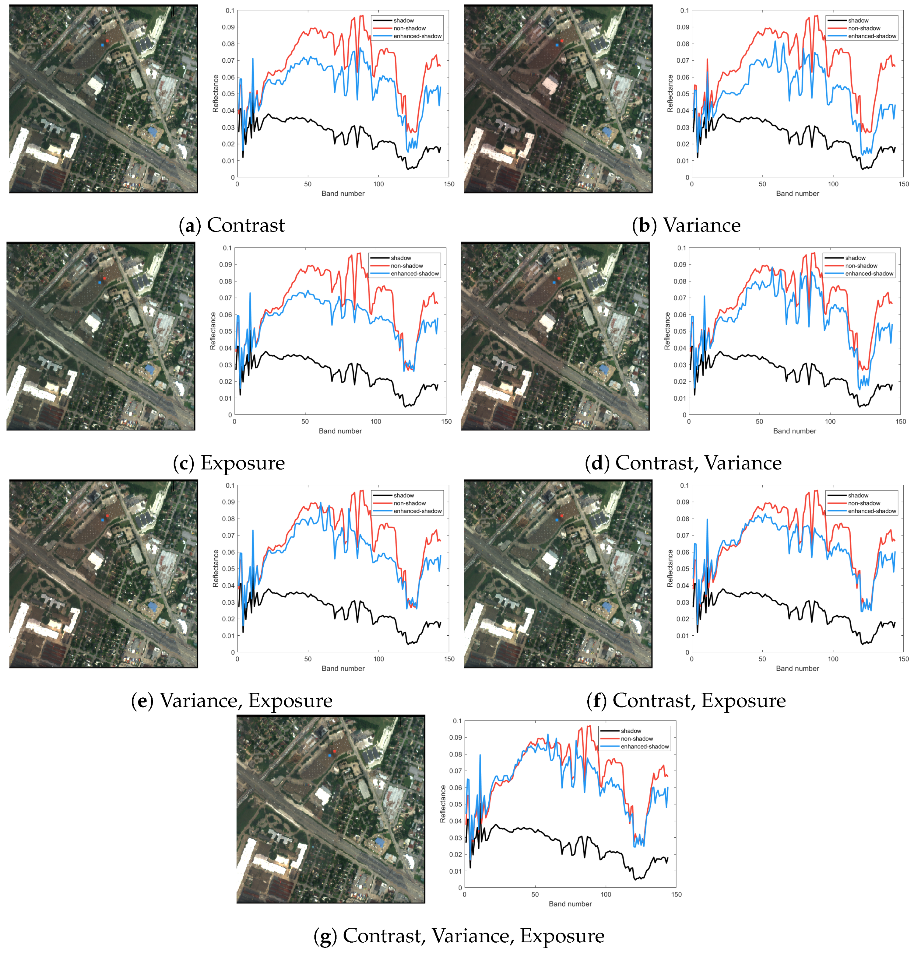
- We introduce a shadow compensation method for hyperspectral images utilizing multi-exposure fusion. This method adaptively computes exposure coefficients and effectively merges exposure sequences by employing spectral variance as the fusion weight, thus mitigating nonlinear attenuation in shadow regions.
- We propose an edge fusion method using the p-Laplacian operator to achieve smooth transitions and seamless merging between shadowed and non-shadowed areas.
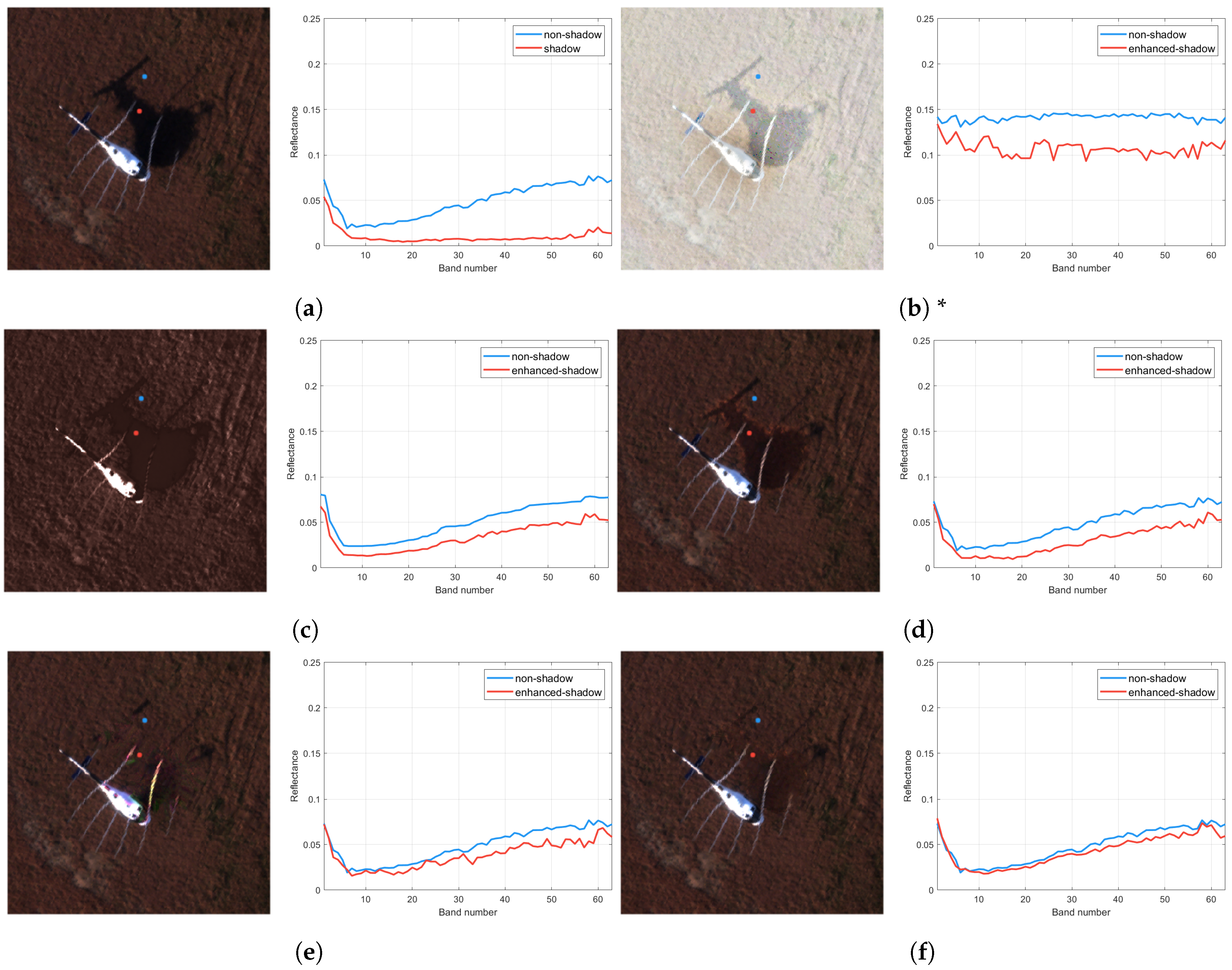
- To address the issue that existing datasets cannot evaluate spectral fidelity after shadow compensation, we develop a hyperspectral image dataset with a uniform background to validate different methods using spectral similarity metrics.
- Experimental results from both the public and proposed dataset demonstrate that our method can effectively compensate shadows, improving classification performance in hyperspectral images.
2. Related Work
2.1. Shadow Detection
2.2. Shadow Compensation
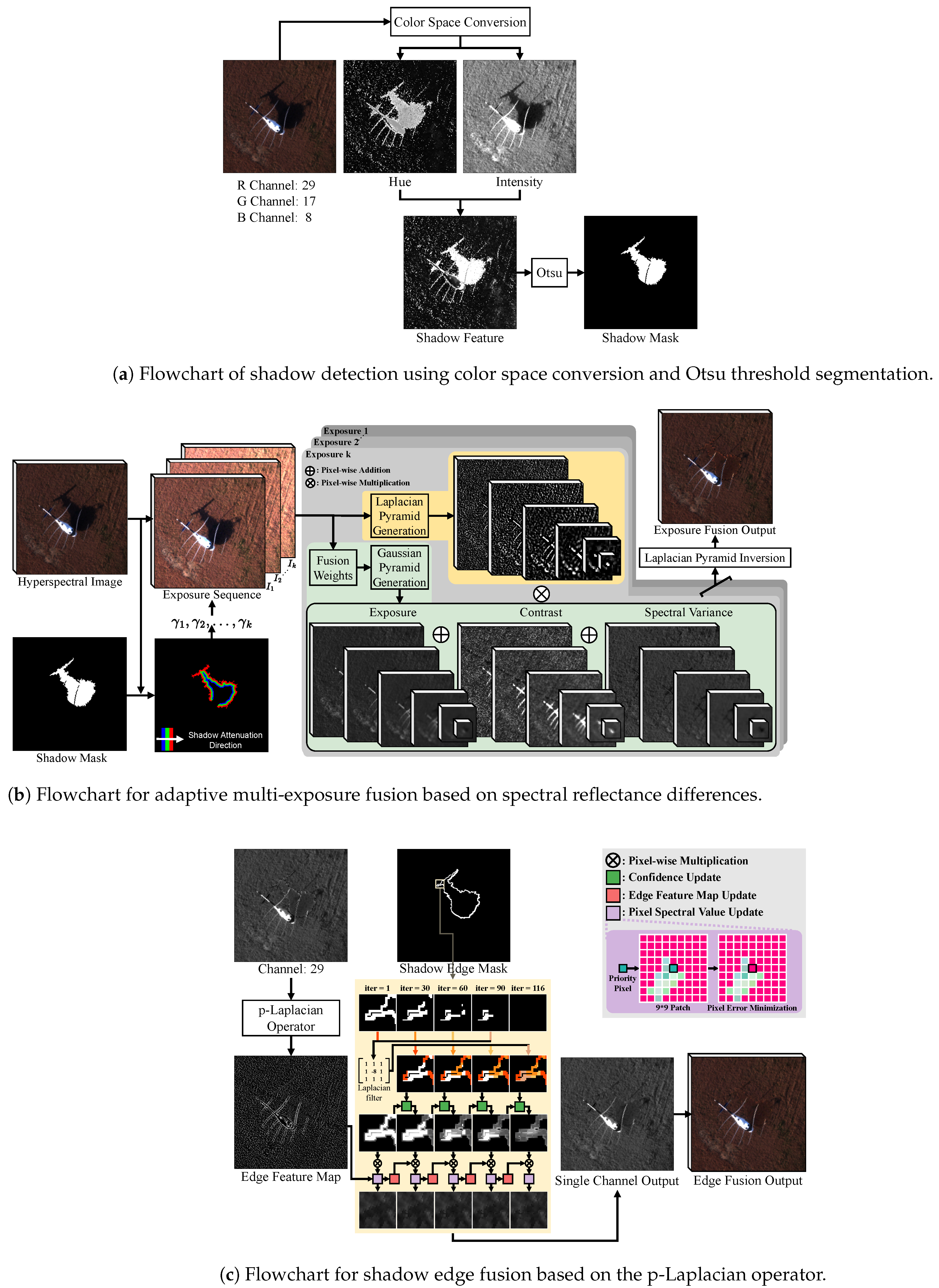
3. Method
3.1. Overall Architecture
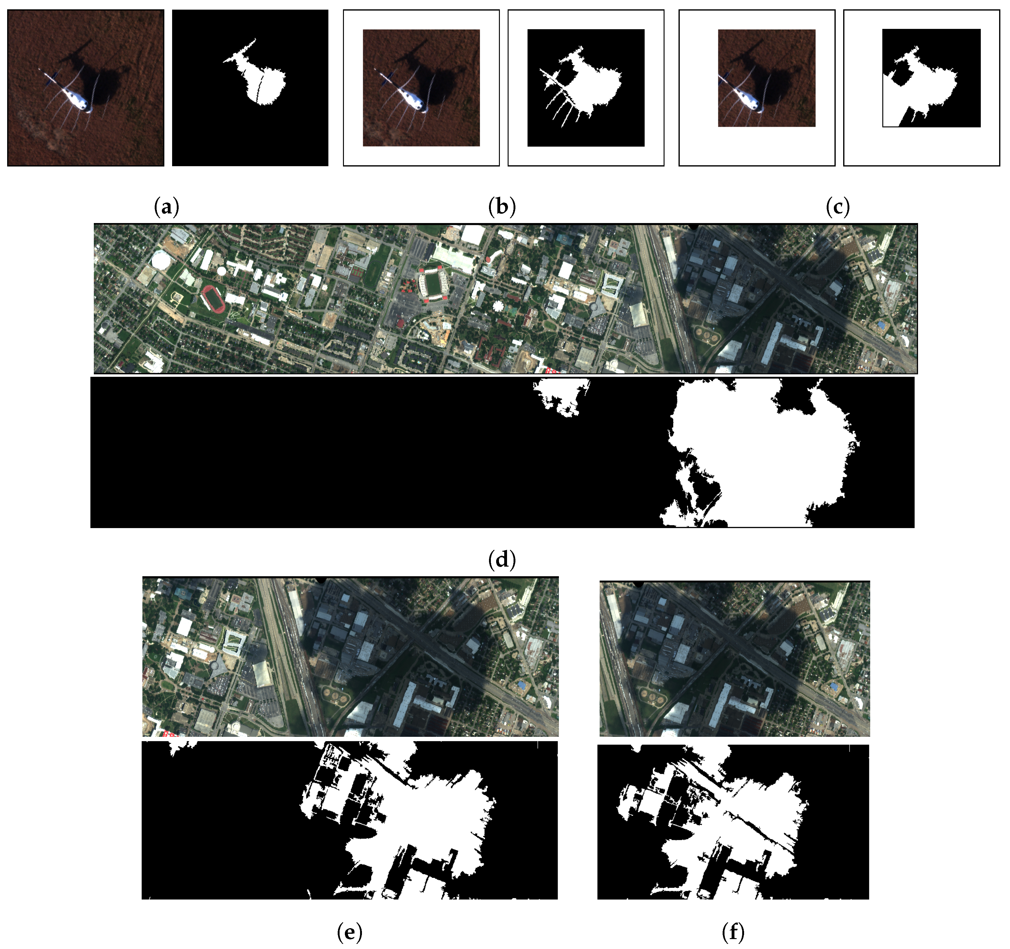
3.2. Shadow Detection
3.3. Shadow Compensation
3.3.1. Multi-Exposure Fusion
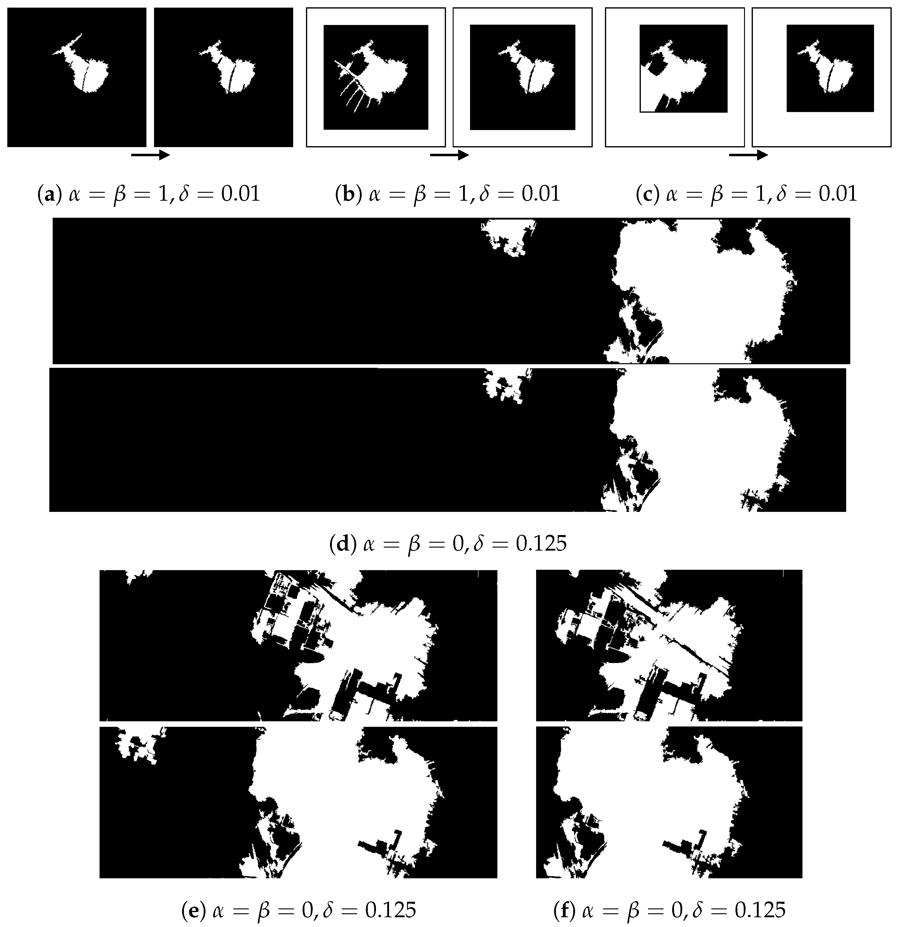
3.3.2. Edge Fusion
| Algorithm 1 Edge fusion algorithm |
|
4. Experiment
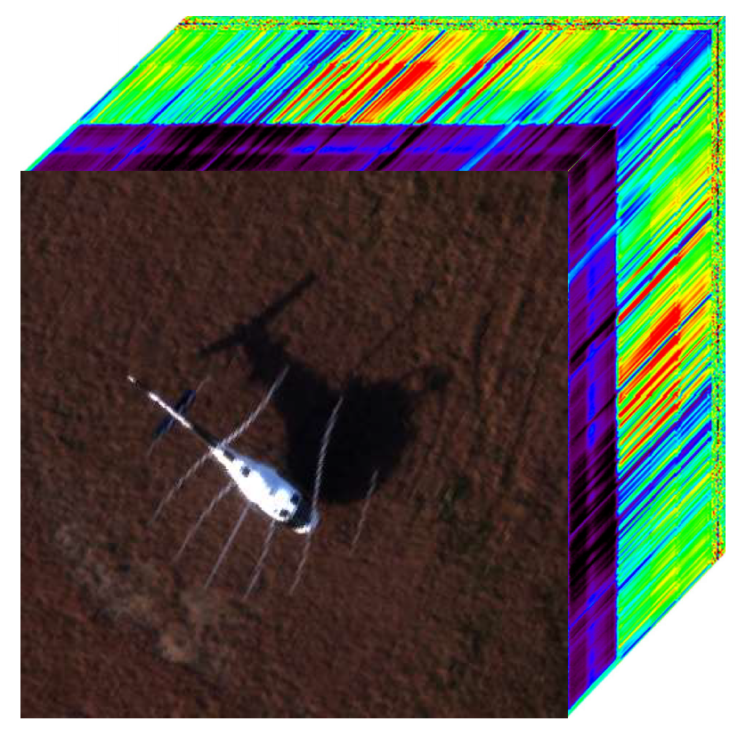
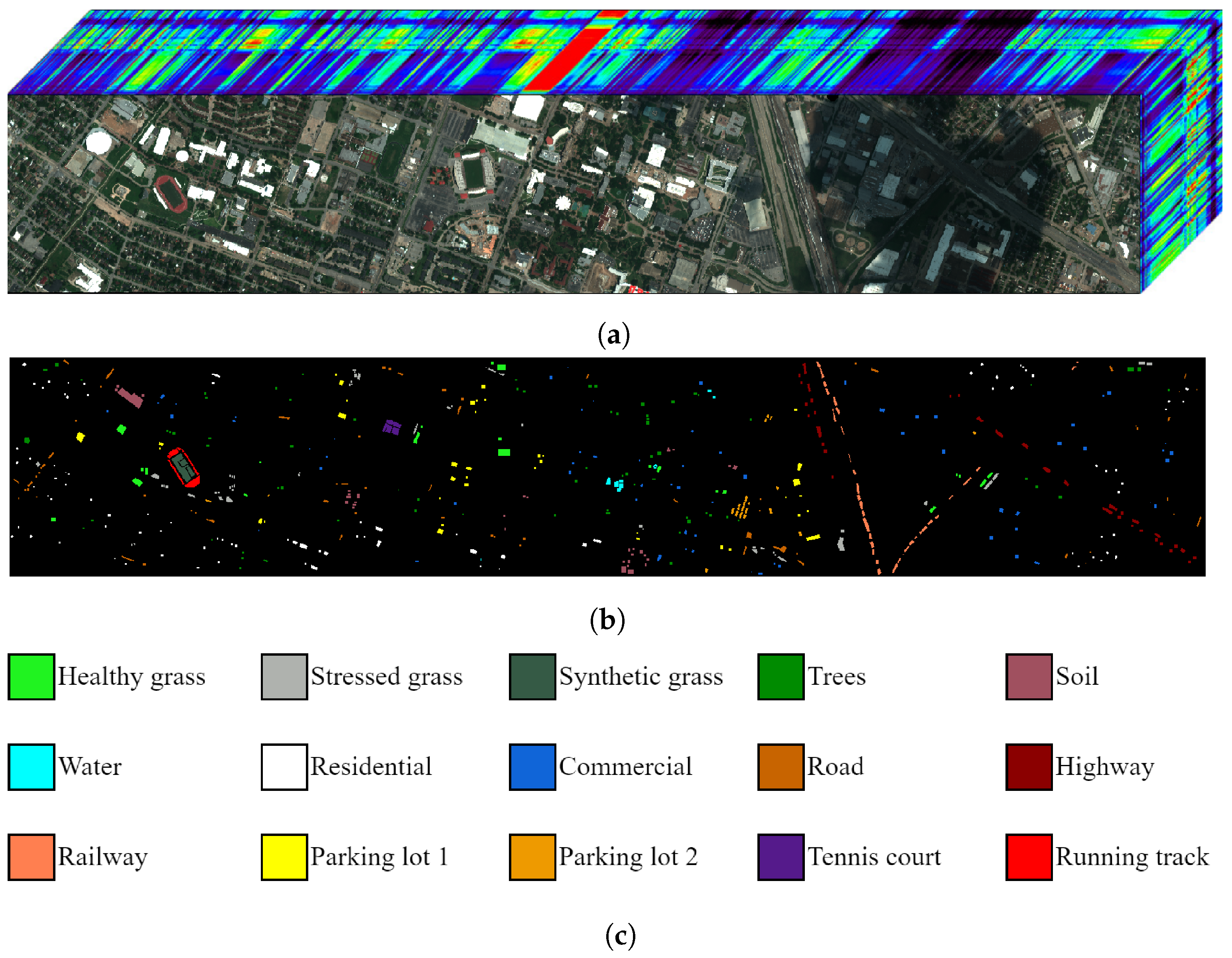
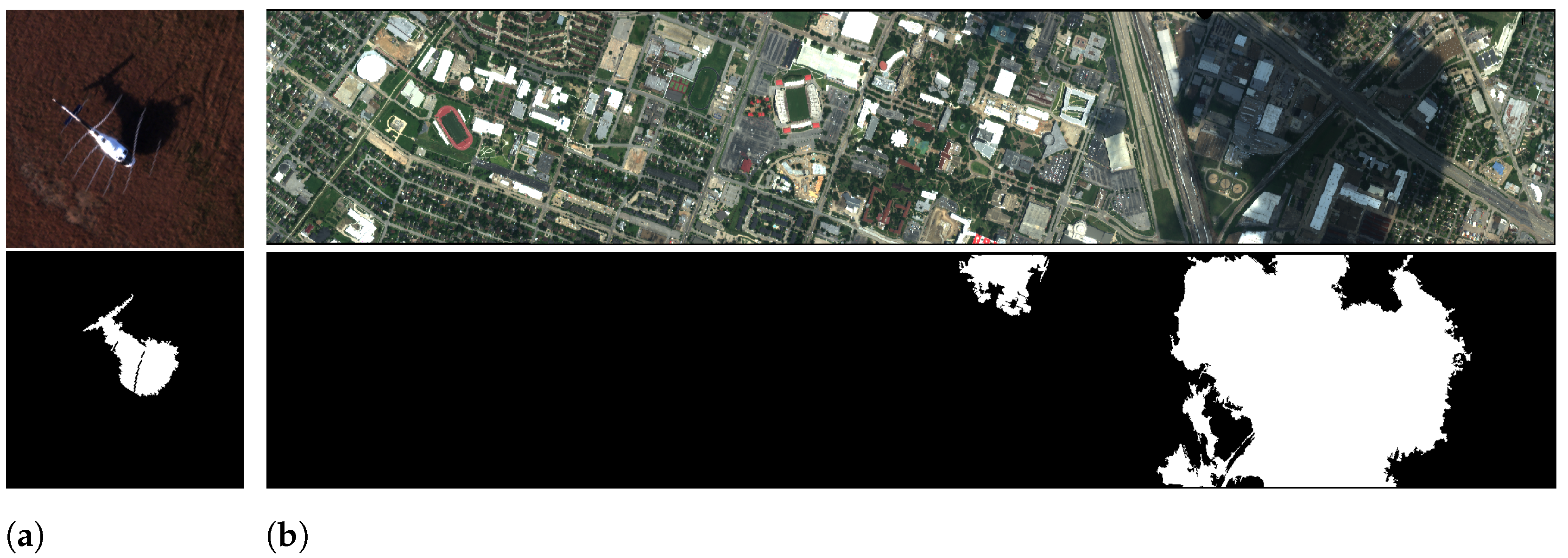
4.1. Dataset
4.1.1. Airport Dataset
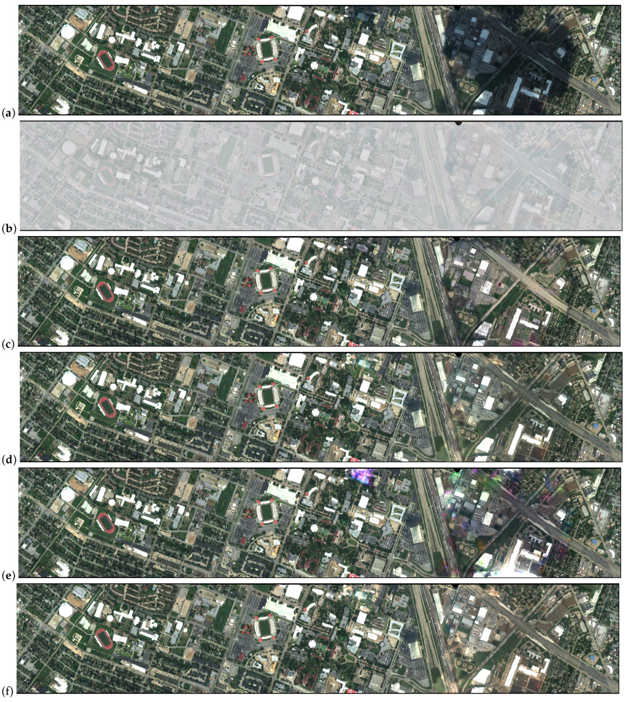
4.1.2. Houston Dataset
4.2. Evaluation Metrics
4.2.1. Classification Evaluation
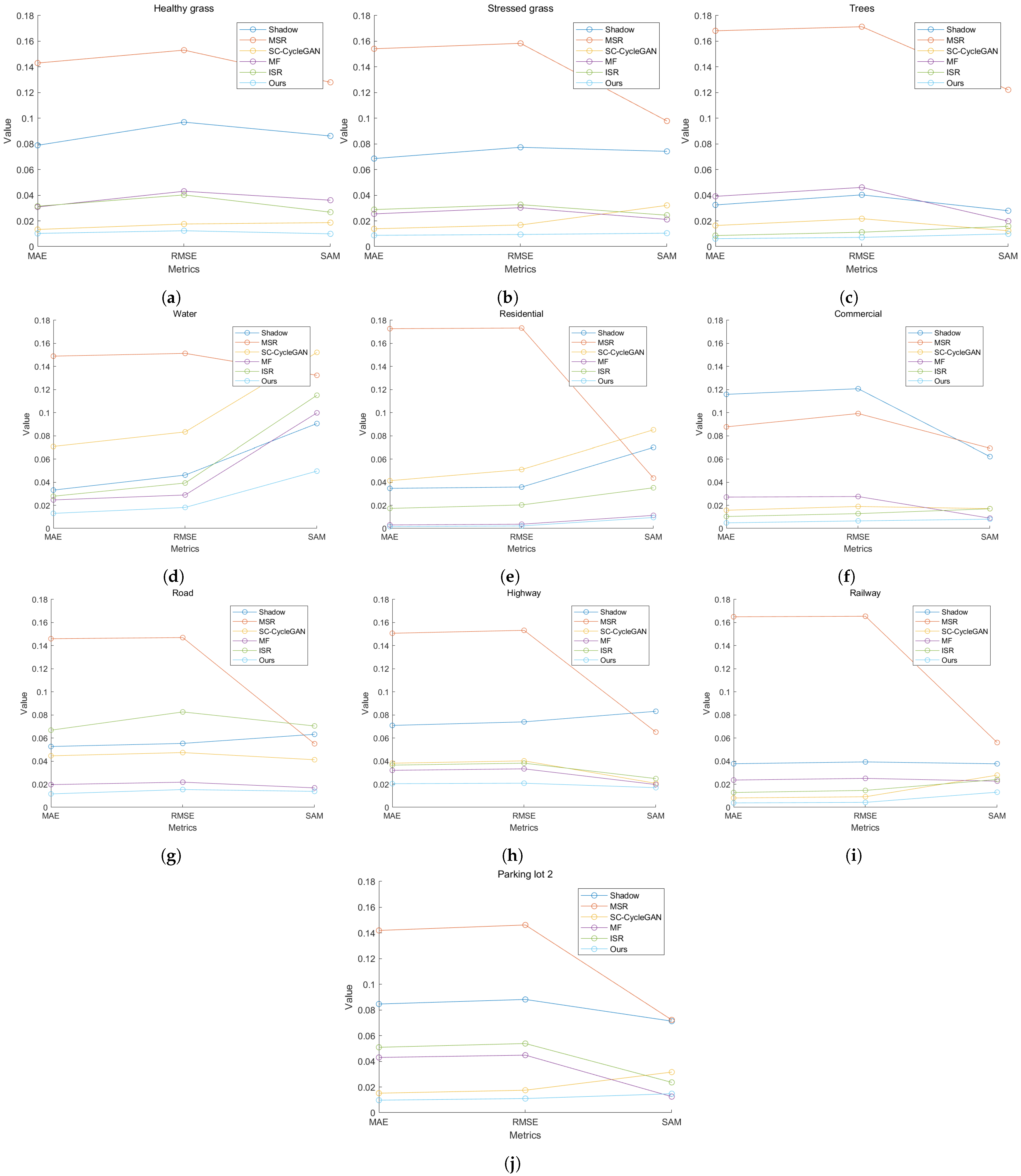
4.2.2. Spectral Similarity
4.3. Implementation Details
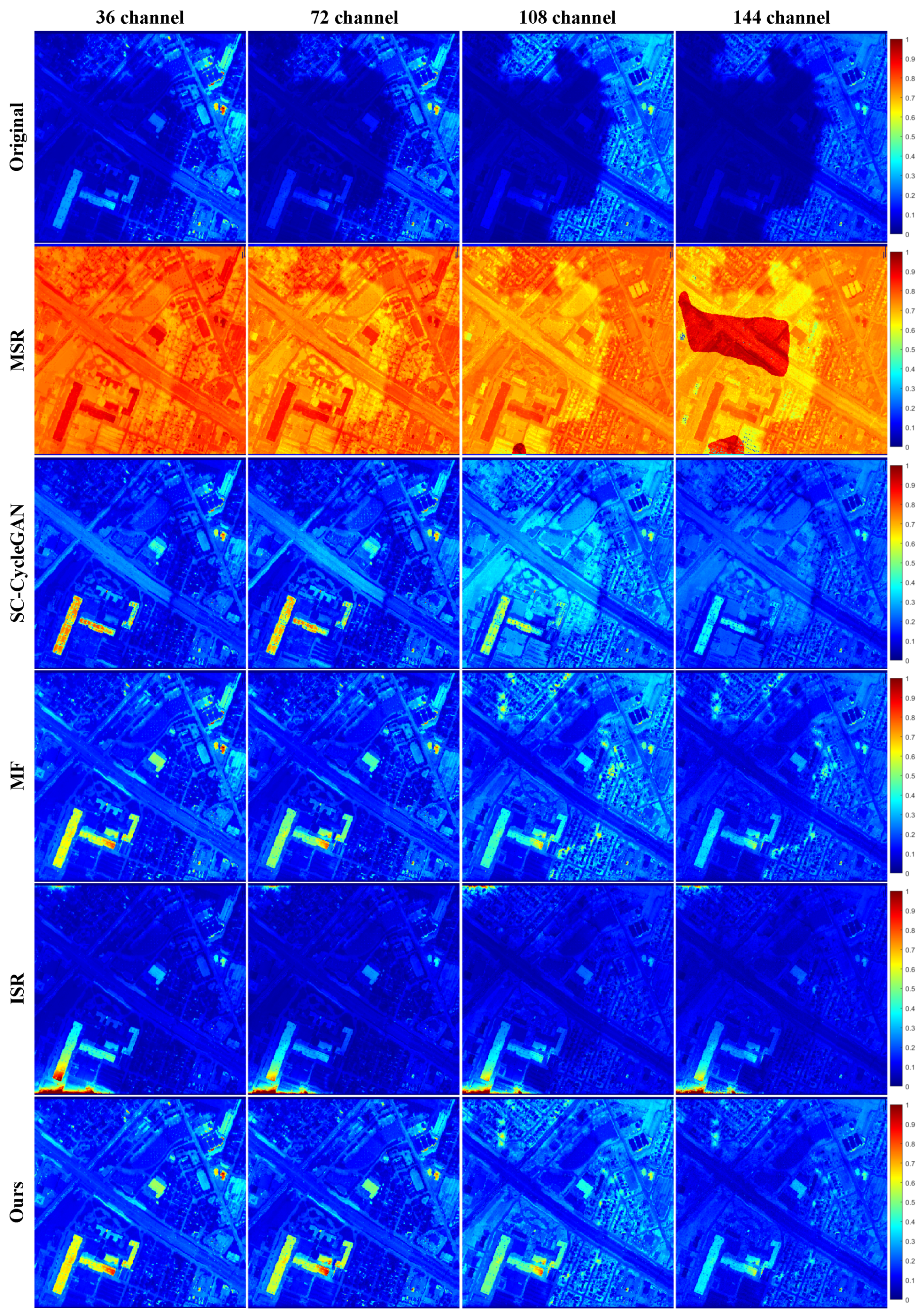
4.4. Results Discussion
4.5. Discussion of Limitations and Future Analysis
5. Conclusions
Author Contributions
Funding
Institutional Review Board Statement
Informed Consent Statement
Data Availability Statement
Acknowledgments
Conflicts of Interest
Abbreviations
| NIR | Near-infrared |
| CycleGAN | Cycle-Consistent Generative Adversarial Network |
| IOOPL | Inner-Outer Outline Profile Line |
| SC-CycleGAN | Shadow compensation via cycle-consistent adversarial networks |
| HSI | Hue, Saturation, and Intensity |
| TAM | Tricolor Attenuation Model |
| DSM | Digital Surface Model |
| SVM | Support Vector Machine |
| GMM | Gaussian Mixture Models |
| GRSS | IEEE Geoscience and Remote Sensing Society |
| OA | Overall Accuracy |
| AA | Average Accuracy |
| MAE | Mean Absolute Error |
| RMSE | Root Mean Squared Error |
| SAM | Spectral Angle Mapper |
| MSR | Multi-scale Retinex |
| MF | Multi-exposure Fusion |
| ISR | Interactive shadow removal |
References
- ElMasry, G.; Sun, D.W. Principles of hyperspectral imaging technology. In Hyperspectral Imaging for Food Quality Analysis and Control; Elsevier: Amsterdam, The Netherlands, 2010; pp. 3–43. [Google Scholar] [CrossRef]
- Landgrebe, D. Hyperspectral image data analysis. IEEE Signal Process. Mag. 2002, 19, 17–28. [Google Scholar] [CrossRef]
- Goetz, A.F.; Vane, G.; Solomon, J.E.; Rock, B.N. Imaging spectrometry for earth remote sensing. Science 1985, 228, 1147–1153. [Google Scholar] [CrossRef]
- Dale, L.M.; Thewis, A.; Boudry, C.; Rotar, I.; Dardenne, P.; Baeten, V.; Pierna, J.A.F. Hyperspectral imaging applications in agriculture and agro-food product quality and safety control: A review. Appl. Spectrosc. Rev. 2013, 48, 142–159. [Google Scholar] [CrossRef]
- Zhang, B.; Wu, D.; Zhang, L.; Jiao, Q.; Li, Q. Application of hyperspectral remote sensing for environment monitoring in mining areas. Environ. Earth Sci. 2012, 65, 649–658. [Google Scholar] [CrossRef]
- Yuen, P.W.; Richardson, M. An introduction to hyperspectral imaging and its application for security, surveillance and target acquisition. Imaging Sci. J. 2010, 58, 241–253. [Google Scholar] [CrossRef]
- Qiao, X.; Yuan, D.; Li, H. Urban shadow detection and classification using hyperspectral image. J. Indian Soc. Remote Sens. 2017, 45, 945–952. [Google Scholar] [CrossRef]
- Duan, P.; Hu, S.; Kang, X.; Li, S. Shadow removal of hyperspectral remote sensing images with multiexposure fusion. IEEE Trans. Geosci. Remote Sens. 2022, 60, 1–11. [Google Scholar] [CrossRef]
- Fredembach, C.; Süsstrunk, S. Automatic and Accurate Shadow Detection from (Potentially) a Single Image Using Near-Infrared Information. 2010. Available online: https://infoscience.epfl.ch/record/165527 (accessed on 28 October 2023).
- Richter, R.; Müller, A. De-shadowing of satellite/airborne imagery. Int. J. Remote Sens. 2005, 26, 3137–3148. [Google Scholar] [CrossRef]
- Dare, P.M. Shadow analysis in high-resolution satellite imagery of urban areas. Photogramm. Eng. Remote Sens. 2005, 71, 169–177. [Google Scholar] [CrossRef]
- Zhang, H.; Sun, K.; Li, W. Object-oriented shadow detection and removal from urban high-resolution remote sensing images. IEEE Trans. Geosci. Remote Sens. 2014, 52, 6972–6982. [Google Scholar] [CrossRef]
- Wang, Q.; Yan, L.; Yuan, Q.; Ma, Z. An automatic shadow detection method for VHR remote sensing orthoimagery. Remote Sens. 2017, 9, 469. [Google Scholar] [CrossRef]
- Zhou, T.; Fu, H.; Sun, C.; Wang, S. Shadow detection and compensation from remote sensing images under complex urban conditions. Remote Sens. 2021, 13, 699. [Google Scholar] [CrossRef]
- Zhao, M.; Chen, J.; Rahardja, S. Hyperspectral shadow removal via nonlinear unmixing. IEEE Geosci. Remote Sens. Lett. 2020, 18, 881–885. [Google Scholar] [CrossRef]
- Zhao, M.; Yan, L.; Chen, J. Hyperspectral image shadow compensation via cycle-consistent adversarial networks. Neurocomputing 2021, 450, 61–69. [Google Scholar] [CrossRef]
- Windrim, L.; Ramakrishnan, R.; Melkumyan, A.; Murphy, R.J. A physics-based deep learning approach to shadow invariant representations of hyperspectral images. IEEE Trans. Image Process. 2017, 27, 665–677. [Google Scholar] [CrossRef] [PubMed]
- Roper, T.; Andrews, M. Shadow modelling and correction techniques in hyperspectral imaging. Electron. Lett. 2013, 49, 458–460. [Google Scholar] [CrossRef]
- Arévalo, V.; González, J.; Ambrosio, G. Shadow detection in colour high-resolution satellite images. Int. J. Remote Sens. 2008, 29, 1945–1963. [Google Scholar] [CrossRef]
- Tian, J.; Sun, J.; Tang, Y. Tricolor attenuation model for shadow detection. IEEE Trans. Image Process. 2009, 18, 2355–2363. [Google Scholar] [CrossRef]
- Huang, J.; Xie, W.; Tang, L. Detection of and compensation for shadows in colored urban aerial images. In Proceedings of the Fifth World Congress on Intelligent Control and Automation (IEEE Cat. No. 04EX788), Hangzhou, China, 15–19 June 2004; IEEE: New York, NY, USA, 2004; Volume 4, pp. 3098–3100. [Google Scholar] [CrossRef]
- Tsai, V.J. A comparative study on shadow compensation of color aerial images in invariant color models. IEEE Trans. Geosci. Remote Sens. 2006, 44, 1661–1671. [Google Scholar] [CrossRef]
- Tolt, G.; Shimoni, M.; Ahlberg, J. A shadow detection method for remote sensing images using VHR hyperspectral and LIDAR data. In Proceedings of the 2011 IEEE International Geoscience and Remote Sensing Symposium, Vancouver, BC, Canada, 24–29 July 2011; IEEE: New York, NY, USA, 2011; pp. 4423–4426. [Google Scholar] [CrossRef]
- Li, Y.; Gong, P.; Sasagawa, T. Integrated shadow removal based on photogrammetry and image analysis. Int. J. Remote Sens. 2005, 26, 3911–3929. [Google Scholar] [CrossRef]
- Martel-Brisson, N.; Zaccarin, A. Moving cast shadow detection from a gaussian mixture shadow model. In Proceedings of the 2005 IEEE Computer Society Conference on Computer Vision and Pattern Recognition (CVPR’05), San Diego, CA, USA, 20–25 June 2005; IEEE: New York, NY, USA, 2005; Volume 2, pp. 643–648. [Google Scholar]
- Wu, T.P.; Tang, C.K. A bayesian approach for shadow extraction from a single image. In Proceedings of the Tenth IEEE International Conference on Computer Vision (ICCV’05) Volume 1, Beijing, China, 17–21 October 2005; IEEE: New York, NY, USA, 2005; Volume 1, pp. 480–487. [Google Scholar] [CrossRef]
- Zhan, Q.; Shi, W.; Xiao, Y. Quantitative analysis of shadow effects in high-resolution images of urban areas. Int. Arch. Photogramm. Remote Sens. 2005, 36, 1–6. [Google Scholar]
- Zhou, W.; Huang, G.; Troy, A.; Cadenasso, M. Object-based land cover classification of shaded areas in high spatial resolution imagery of urban areas: A comparison study. Remote Sens. Environ. 2009, 113, 1769–1777. [Google Scholar] [CrossRef]
- Liu, Y.; Bioucas-Dias, J.; Li, J.; Plaza, A. Hyperspectral cloud shadow removal based on linear unmixing. In Proceedings of the 2017 IEEE International Geoscience and Remote Sensing Symposium (IGARSS), Fort Worth, TX, USA, 23–28 July 2017; IEEE: New York, NY, USA, 2017; pp. 1000–1003. [Google Scholar] [CrossRef]
- Zhang, G.; Cerra, D.; Müller, R. Shadow detection and restoration for hyperspectral images based on nonlinear spectral unmixing. Remote Sens. 2020, 12, 3985. [Google Scholar] [CrossRef]
- Yamazaki, F.; Liu, W.; Takasaki, M. Characteristics of shadow and removal of its effects for remote sensing imagery. In Proceedings of the 2009 IEEE International Geoscience and Remote Sensing Symposium, Cape Town, South Africa, 12–17 July 2009; IEEE: New York, NY, USA, 2009; Volume 4, pp. IV–426. [Google Scholar] [CrossRef]
- Finlayson, G.D.; Hordley, S.D.; Lu, C.; Drew, M.S. On the removal of shadows from images. IEEE Trans. Pattern Anal. Mach. Intell. 2005, 28, 59–68. [Google Scholar] [CrossRef] [PubMed]
- Hartzell, P.; Glennie, C.; Khan, S. Terrestrial hyperspectral image shadow restoration through lidar fusion. Remote Sens. 2017, 9, 421. [Google Scholar] [CrossRef]
- Jia, S.; Jiang, S.; Lin, Z.; Li, N.; Xu, M.; Yu, S. A survey: Deep learning for hyperspectral image classification with few labeled samples. Neurocomputing 2021, 448, 179–204. [Google Scholar] [CrossRef]
- He, J.; Yuan, Q.; Li, J.; Xiao, Y.; Liu, D.; Shen, H.; Zhang, L. Spectral super-resolution meets deep learning: Achievements and challenges. Inf. Fusion 2023, 97, 101812. [Google Scholar] [CrossRef]
- Friman, O.; Tolt, G.; Ahlberg, J. Illumination and shadow compensation of hyperspectral images using a digital surface model and non-linear least squares estimation. In Proceedings of the Image and Signal Processing for Remote Sensing XVII; SPIE: Bellingham, WA, USA, 2011; Volume 8180, pp. 183–190. [Google Scholar] [CrossRef]
- Uezato, T.; Yokoya, N.; He, W. Illumination invariant hyperspectral image unmixing based on a digital surface model. IEEE Trans. Image Process. 2020, 29, 3652–3664. [Google Scholar] [CrossRef] [PubMed]
- Kang, X.; Huang, Y.; Li, S.; Lin, H.; Benediktsson, J.A. Extended random walker for shadow detection in very high resolution remote sensing images. IEEE Trans. Geosci. Remote Sens. 2017, 56, 867–876. [Google Scholar] [CrossRef]
- Otsu, N. A threshold selection method from gray-level histograms. IEEE Trans. Syst. Man Cybern. 1979, 9, 62–66. [Google Scholar] [CrossRef]
- Mertens, T.; Kautz, J.; Van Reeth, F. Exposure fusion: A simple and practical alternative to high dynamic range photography. In Proceedings of the Computer Graphics Forum; Wiley Online Library: Oxford, UK, 2009; Volume 28, pp. 161–171. [Google Scholar] [CrossRef]
- Melgani, F.; Bruzzone, L. Classification of hyperspectral remote sensing images with support vector machines. IEEE Trans. Geosci. Remote Sens. 2004, 42, 1778–1790. [Google Scholar] [CrossRef]
- Kruse, F.A.; Lefkoff, A.; Boardman, J.; Heidebrecht, K.; Shapiro, A.; Barloon, P.; Goetz, A. The spectral image processing system (SIPS)—interactive visualization and analysis of imaging spectrometer data. Remote Sens. Environ. 1993, 44, 145–163. [Google Scholar] [CrossRef]
- Lin, H.; Shi, Z. Multi-scale retinex improvement for nighttime image enhancement. Optik 2014, 125, 7143–7148. [Google Scholar] [CrossRef]
- Gong, H.; Cosker, D. Interactive removal and ground truth for difficult shadow scenes. JOSA A 2016, 33, 1798–1811. [Google Scholar] [CrossRef] [PubMed]

| Metrics | Original | MSR | SC-Cyc. | MF | ISR | Ours |
|---|---|---|---|---|---|---|
| MAE (20 px) | 0.0344 | 0.1299 | 0.0114 | 0.0150 | 0.0113 | 0.0082 |
| RMSE (20 px) | 0.0382 | 0.1383 | 0.0119 | 0.0159 | 0.0131 | 0.0099 |
| SAM (20 px) | 0.6867 | 0.0856 | 0.0598 | 0.1789 | 0.1655 | 0.0490 |
| MAE (50 px) | 0.0333 | 0.1362 | 0.0089 | 0.0137 | 0.0103 | 0.0077 |
| RMSE (50 px) | 0.0369 | 0.1462 | 0.0094 | 0.0146 | 0.0122 | 0.0094 |
| SAM (50 px) | 0.6702 | 0.0984 | 0.0513 | 0.1725 | 0.1615 | 0.0500 |
| MAE (100 px) | 0.0346 | 0.1394 | 0.0101 | 0.0140 | 0.0102 | 0.0078 |
| RMSE (100 px) | 0.0383 | 0.1497 | 0.0106 | 0.0149 | 0.0121 | 0.0095 |
| SAM (100 px) | 0.6760 | 0.0988 | 0.0550 | 0.1749 | 0.1628 | 0.0511 |
| Accuracies of Non-Shadowed (%) | Accuracies of Shadowed (%) | |||||||||||
|---|---|---|---|---|---|---|---|---|---|---|---|---|
| Class Name | Origi. | MSR | SC-Cyc. | MF | ISR | Ours | Origi. | MSR | SC-Cyc. | MF | ISR | Ours |
| Healthy grass | 98.08 | 0.00 | 97.75 | 97.81 | 97.91 | 97.86 | 12.92 | 0.00 | 25.28 | 54.49 | 16.85 | 51.12 |
| Stressed grass | 98.27 | 0.00 | 98.32 | 98.43 | 98.38 | 98.22 | 18.29 | 0.00 | 32.93 | 54.88 | 47.56 | 75.00 |
| Synthetic grass | 88.46 | 0.00 | 88.49 | 88.79 | 88.46 | 88.03 | - | - | - | - | - | - |
| Trees | 98.12 | 0.00 | 97.96 | 98.37 | 98.38 | 98.17 | 41.13 | 0.00 | 42.74 | 75.00 | 37.10 | 67.74 |
| Soil | 91.42 | 0.00 | 91.46 | 86.15 | 85.25 | 91.82 | - | - | - | - | - | - |
| Water | 98.11 | 0.00 | 98.11 | 97.67 | 97.67 | 98.53 | 12.50 | 0.00 | 5.00 | 2.50 | 0.00 | 22.50 |
| Residential | 72.73 | 0.00 | 72.76 | 75.27 | 74.73 | 71.79 | 10.00 | 0.00 | 16.25 | 51.25 | 18.75 | 71.25 |
| Commercial | 55.34 | 11.19 | 54.51 | 55.84 | 56.14 | 55.72 | 53.73 | 0.00 | 69.96 | 71.49 | 70.61 | 74.78 |
| Road | 67.48 | 0.00 | 67.39 | 66.86 | 66.69 | 68.19 | 8.11 | 18.92 | 2.70 | 29.73 | 16.22 | 56.76 |
| Highway | 43.68 | 0.00 | 43.34 | 45.11 | 43.93 | 43.55 | 4.29 | 0.00 | 3.07 | 78.53 | 6.13 | 85.28 |
| Railway | 60.61 | 0.00 | 61.01 | 53.22 | 51.34 | 60.34 | 3.91 | 0.00 | 3.26 | 47.88 | 8.14 | 67.10 |
| Parking lot 1 | 48.16 | 0.00 | 48.17 | 49.13 | 47.80 | 47.88 | - | - | - | - | - | - |
| Parking lot 2 | 15.46 | 0.00 | 13.20 | 16.35 | 17.23 | 16.35 | 0.00 | 5.00 | 0.00 | 10.00 | 5.00 | 15.00 |
| Tennis court | 85.64 | 0.00 | 85.19 | 85.89 | 85.61 | 85.08 | - | - | - | - | - | - |
| Running track | 99.10 | 0.00 | 99.02 | 89.97 | 98.31 | 99.11 | - | - | - | - | - | - |
| OA | 77.12 | 5.93 | 77.05 | 76.43 | 75.96 | 77.09 | 22.58 | 0.46 | 29.27 | 61.43 | 31.35 | 70.03 |
| AA | 71.30 | 6.25 | 71.18 | 70.65 | 70.30 | 71.32 | 16.49 | 2.39 | 20.12 | 47.58 | 22.64 | 58.65 |
| Kappa | 75.22 | 0.00 | 75.14 | 74.47 | 73.96 | 75.18 | 7.38 | 0.00 | 15.39 | 53.86 | 17.88 | 64.15 |
| Datasets | MSR | SC-Cyc. | MF | ISR | Ours 1 | Ours 2 |
|---|---|---|---|---|---|---|
| Airport | 68.21 | 2375.14 | 13.22 | 921.35 | 19.25 | 8.17 |
| Houston | 237.31 | 101,723.52 | 172.48 | 6632.19 | 234.23 | 101.18 |
Disclaimer/Publisher’s Note: The statements, opinions and data contained in all publications are solely those of the individual author(s) and contributor(s) and not of MDPI and/or the editor(s). MDPI and/or the editor(s) disclaim responsibility for any injury to people or property resulting from any ideas, methods, instructions or products referred to in the content. |
© 2024 by the authors. Licensee MDPI, Basel, Switzerland. This article is an open access article distributed under the terms and conditions of the Creative Commons Attribution (CC BY) license (https://creativecommons.org/licenses/by/4.0/).
Share and Cite
Meng, Y.; Li , G.; Huang, W. Adaptive Shadow Compensation Method in Hyperspectral Images via Multi-Exposure Fusion and Edge Fusion. Appl. Sci. 2024, 14, 3890. https://doi.org/10.3390/app14093890
Meng Y, Li G, Huang W. Adaptive Shadow Compensation Method in Hyperspectral Images via Multi-Exposure Fusion and Edge Fusion. Applied Sciences. 2024; 14(9):3890. https://doi.org/10.3390/app14093890
Chicago/Turabian StyleMeng, Yan, Guanyi Li , and Wei Huang. 2024. "Adaptive Shadow Compensation Method in Hyperspectral Images via Multi-Exposure Fusion and Edge Fusion" Applied Sciences 14, no. 9: 3890. https://doi.org/10.3390/app14093890
APA StyleMeng, Y., Li , G., & Huang, W. (2024). Adaptive Shadow Compensation Method in Hyperspectral Images via Multi-Exposure Fusion and Edge Fusion. Applied Sciences, 14(9), 3890. https://doi.org/10.3390/app14093890