Fatigue Crack and Residual Life Prediction Based on an Adaptive Dynamic Bayesian Network

Abstract

Monitoring the health status of aerospace structures during their service lives is a critical endeavor, aimed at precisely evaluating their operational condition through observation data and physical modeling. This study proposes a probabilistic assessment approach utilizing Dynamic Bayesian Networks (DBNs), enhanced by an improved adaptive particle filtering technique. This approach combines physical modeling with various predictive sources, encompassing cognitive uncertainties inherent in stochastic predictions and crack propagation forecasts. By employing crack observation data, it facilitates predictions of crack growth and the residual life of metal structure. To demonstrate the efficacy of this method, the research leverages data from three-point bending and single-edge tension fatigue tests. It gathers data on crack length during the fatigue crack progression, integrating these findings with digital twin theory to forecast the residual fatigue life of the specimens. The outcomes show that the adaptive DBN model can precisely predict fatigue crack propagation in test specimens, offering a potential tool for the online health assessment and life evaluation for aerospace structures.

1. Introduction

Modern aerospace vehicles must withstand complex service environments, posing an increasingly strict requirement for structural performance. As the service load condition becomes severer, coupled with inevitable defects and residual stresses from manufacturing processes, the degradation of material and structural performance is an issue that cannot be ignored. The harsh service environment can generate structural damage in terms of cracks, delamination, etc., which poses a serious threat to structural safety and integrity. On the other hand, the reusability of aerospace structures has been a core concern in recent years [1]. Reusability is achieved through a combination of a “safety factor + regular maintenance” approach, that is, by increasing the safety margin to enhance structural durability and ensuring reliability through inspections and maintenance [2]. This challenge necessitates a deep understanding of the service environment and load-bearing capacity of structures, as well as effective prediction and management of potential damages. To further enhance the confidence in structural integrity assessments, structural health monitoring technologies for real-time monitoring and evaluation of the service state of structures play a significant role in improving structural performance, ensuring service safety, and reducing maintenance costs [3].

Currently, there are two main methods for structural health monitoring [4]: one is based on artificial intelligence data analysis, and the other is based on physical models (PMs). However, the use of pure data-driven models can be expensive, as it requires costly experiments to obtain data. Meanwhile, simulation-driven PM/FEM models have modeling errors that deviate from actual structures. Practical systems inevitably encounter uncertainties [5], such as sensor noise, material defects, mechanical damage, vibration, and load interference, which can interfere with their diagnostic reasoning and health assessment. Additionally, real-world systems are dynamic and change over time with their health status. Therefore, there is a crucial need to combine physical models with data-driven models to solve health monitoring problems.

Recently, the concept of digital twins has gained widespread attention in the field of intelligent manufacturing due to the development of communication technology in intelligent algorithms [6,7]. Digital twins establish an interactive relationship between the physical and digital worlds. They provide simulation models based on physical mechanisms and health monitoring services for data obtained in the physical world. Complex systems collect sensor data from the physical world and send them to digital twin virtual models through communication technology. The digital twin virtual model processes these data, updates the simulated physical model in real time, and sends control commands to provide optimization and decision support for physical systems.

The U.S. Air Force adopted the “Airframe Digital Twin” (ADT) for aircraft design, maintenance, and performance prediction. It employs digital twins to replicate the physical and mechanical attributes of aircraft, enabling the prediction of structural fatigue cracks and extension of the aircraft’s remaining service life [8,9,10]. The ADT encompasses three core modules: online monitoring, condition assessment, and lifespan prediction. It integrates aerodynamic and finite element analyses along with other structural models, which monitor the evolution of fatigue, vibration, and other material states in flight structures. Through dynamic updates incorporating specific geometry, material properties, flight history, and maintenance data, the ADT precisely forecasts aircraft behavior. This allows decision-makers to tailor personalized management strategies for each aircraft, thereby prolonging service life and reducing maintenance expenses.

Various types of sensors are utilized within the monitoring data collection module of ADT systems for the identification of damage, including ultrasonic sensors, X-ray devices, piezoelectric sensors, fiber Bragg gratings, and distributed fiber optics [11,12,13,14,15]. These sophisticated sensing devices enable the timely detection of crack damages, thus providing a robust guarantee for the safety assessment of structures.

However, due to uncertainties associated with, e.g., material geometry, internal defects, irregular damages, and mechanical environments, the prediction of damage evolution in aerospace structures exhibits unsatisfactory accuracy. Therefore, it is necessary to establish a probabilistic model that integrates diagnosis and prediction, which can reduce the uncertainty of time-independent state variables through continuous observation (diagnosis) and probabilistically predicts the evolution of future crack damages (prognosis), thereby obtaining a more accurate assessment of the structural health state with multiple sources of uncertainty.

Within the digital twin framework, the Dynamic Bayesian Network (DBN) is among the most widely applied probabilistic methods [16,17]. Its robust system reliability framework makes it a primary method for representing and managing uncertainties in physical models (related to geometry, materials, connection stiffness, etc.) in digital twins. DBNs excel at providing direct representations of complex systems and are highly effective in identifying inter-component relationships, making them suitable for monitoring, diagnosis, and prediction tasks in uncertain environments. A unique advantage of DBNs is their ability to integrate a wide range of information sources, including experimental data, historical records, and expert opinions, which is particularly valuable in fault-tolerant systems where data are often sparse and varied. Additionally, DBNs stand out for their capability to model the temporal dynamics of cascading events, offering a more accurate description of how systems evolve over time. This enhances prediction accuracy and aids in better decision-making, resource planning, and allocation in complex and evolving systems.

Wei et al. [18] proposed an object-oriented modeling approach, building a DBN for the entire aviation system health in a bottom–up manner based on Bayesian theory, and validated its effectiveness and robustness through experiments on a specific aviation fuel delivery system. Yu et al. [19] introduced a digital twin health monitoring method based on non-parametric Bayesian networks, combining an improved Gaussian particle filter and a Dirichlet process mixture model for real-time model updating, significantly enhancing monitoring accuracy. Karve et al. [20] developed an intelligent task planning method based on digital twins, employing a DBN to predict the probability distribution of crack propagation, considering the quantification of uncertainties and encompassing damage diagnosis, prediction, and task optimization, to optimize fatigue crack growth and maintenance intervals. Rabiei et al. [21] proposed a DBN framework for the online integration of health assessment information from empirical crack growth models, structural health monitoring, and regular inspections, updating crack size distribution and model parameters for prediction. Boris et al. [22] introduced a framework utilizing a DBN with MCMC for predicting and updating crack length in fatigued structural components, including parameter probability density identification and updating. Lee et al. [23] proposed a Bayesian method to estimate initial crack length distribution for PRA of repaired structures, improving parameter selection and analyzing KT-1 aircraft repair risk.

However, Bayesian networks have some defects. For instance, they are highly dependent on prior probabilities, and prior probabilities often depend on assumptions, leading to poor prediction results. Moreover, the large noise of dynamic measurement data acquisition and the calculation time cost of Bayesian distribution steps make online real-time Bayesian network systems less accurate and precise than offline Bayesian monitoring systems [24], especially for data that are more dependent on manual observation, such as cracks, which are often scarce, and it is challenging to meet the needs of Bayesian networks for a large amount of observation data.

To overcome existing limitations, this study introduces an innovative adaptive DBN model aimed at crafting a predictive module for tracking the evolution of fatigue crack damage in the digital twin systems of aerospace structures. This sophisticated model merges adaptive particle filtering with a comprehensive range of cognitive uncertainties found in crack propagation equations, spanning material characteristics, geometric configurations, model parameters, measurements, and load conditions. It adeptly monitors the progression of time-variant state variables while minimizing uncertainties in time-invariant states (diagnosis). Moreover, the model leverages real-time updates, drawing from calibrated probability distributions of parameters and forecasts, to provide probabilistic estimates of fatigue crack growth and the remaining lifespan (prognosis). Each update introduces new particles to mitigate particle impoverishment, thus ensuring more accurate predictions. The validity and applicability of this model were confirmed using data from three-point bending and single-edge crack fatigue experiments. The findings reveal that the model precisely forecasts the velocity of damage crack progression, offering a feasible tool for the real-time evaluation of structural health and lifespan assessment.

2. Principle and Methods

2.1. Fatigue Crack Growth Theory

In general, the fatigue failure of materials will go through three stages: crack initiation, stable expansion, and rapid unstable failure of cracks. Due to the relatively short time of rapid unstable failure of cracks, the fatigue life is often calculated by selecting the crack initiation life (from the beginning of use to the appearance of engineering detectable cracks) and the crack expansion life (from detectable cracks to critical crack size), as shown in Figure 1.

The mechanism of crack formation life is quite complex. From the beginning of crack nucleation to the point where microscopic cracks expand into macroscopic cracks, it accounts for the largest proportion of fatigue life. Crack nucleation is mainly caused by local stress and strain concentration, and the existence of tiny inclusions or voids in engineering materials has a great influence on the crack nucleation process, resulting in a large degree of discreteness in crack formation life. The length range of microscopic cracks is generally 10–100 μm, which is at the same order of magnitude as the size of the plastic zone at the crack tip. Currently, there are two commonly used methods for estimating crack formation life without obvious macroscopic cracks. The first method is to use the relationship curve between external constant amplitude cyclic stress amplitude S and fatigue life N (referred to as S-N curve) as the main design basis for anti-fatigue design methods. This method has a long history and is still adopted by many anti-fatigue design specifications today. The other method is to assume a reasonable microscopic crack size based on experience (such as a microscopic crack length of 0.0588 inches commonly used in flight structures as the minimum observation size) and use the formula for macroscopic crack extension in fracture mechanics to calculate residual life.

Therefore, whether it is the fatigue life prediction of cracks that assumes reasonable microcrack sizes or the prediction of macroscopic crack fatigue life, it ultimately comes down to the study of the crack propagation rate. Currently, within the category of online elastic fracture mechanics, the strength of the crack tip singularity is characterized by a single parameter, stress intensity factor K. Therefore, many scholars consider linking the fatigue crack propagation rate with K and then propose a series of fatigue crack propagation rate formulas, such as the most basic and commonly used Paris’ law [25], the Forman law [26], and the Walker law [27] that considers the influence of stress ratio R and strength factor threshold K_th, as well as the full crack propagation formula and Nasgro law [28] that integrates simulation software.

According to Paris’ law [25], the crack growth is described by the following:

$$\frac{da}{dN}=\mathrm{C}{\left(\Delta K\right)}^m$$

(1)

where $K=F\sigma \sqrt{\pi a}$ is the stress intensity factor. F is the shape factor. σ is the equivalent stress, which is the stress at the crack location calculated without cracks. a is the crack length. C and m are material parameters determined by experiments. da/dN is the fatigue crack propagation rate. This formula expresses the fatigue crack propagation rate in the form of a power function of the stress intensity factor amplitude ΔK, which describes the law of crack propagation well and has the advantage of convenient calculation. Therefore, it is still widely used in engineering structural fatigue life prediction.

Fatigue crack growth life is the total number of load cycles from the initial crack a₀ to the critical crack length a_c. First, Equation (2) is used to obtain the size of critical crack size a_c.

$$a_c=\frac{1}{\pi }{\left(\frac{K_C}{F{\sigma }_{\max }}\right)}^2$$

(2)

where σ_max is the maximum cyclic stress. K_C is the fracture toughness of the material.

According to crack growth Equation (1), the theoretical formula for predicting residual life is as follows:

$$N={\displaystyle {\int }_{a_0}^{a_c}\frac{da}{C{\left(\Delta K\right)}^m}}$$

(3)

Walker considered the influence of stress amplitude on crack propagation and incorporated the stress ratio R into the Paris’ law, referred to as the Walker law [27], as follows:

$$\frac{da}{dN}=\mathrm{C}{\left({\left(1-R\right)}^{\alpha }\Delta K\right)}^m$$

(4)

However, these laws have some limitations, and the accuracy is different under different crack conditions. For the complex crack conditions in practice, which law can obtain more accurate results is a problem to be solved.

2.2. Brief Introduction to Dynamic Bayesian Network

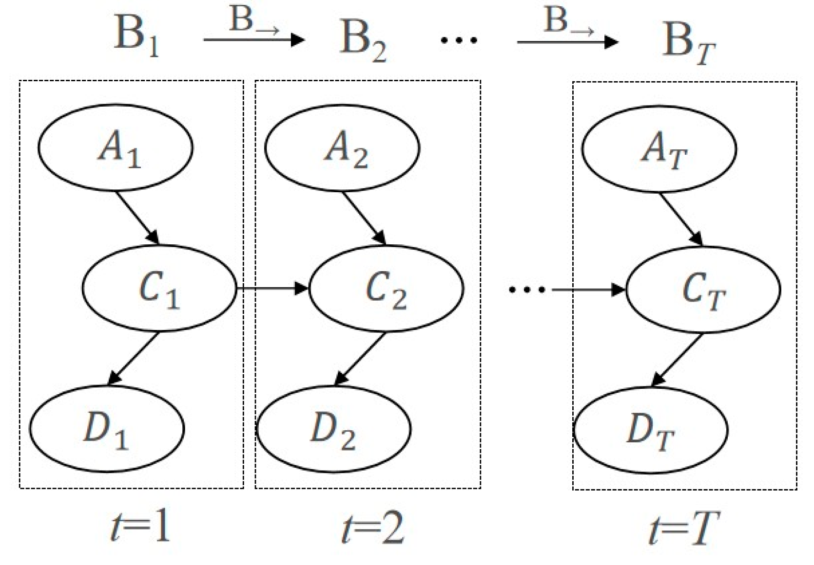
Figure 2 illustrates a simple example of a DBN. Nodes A_i and C_i represent hidden variables, indicating states that cannot be directly observed. In some cases, the variable C_i corresponds to a physical model, and A_i represents parameters of C_i. The node D_i denotes observed variables. The subscripts correspond to different moments. The arrows between nodes describe the conditional dependencies between variables, pointing from parent nodes to child nodes. This directionality from “cause” to “effect” signifies a causal relationship or non-conditional independence between parent and child nodes, which is mathematically characterized by conditional probability distributions (CPDs). Variables with the same subscript form an independent BN, and BNs across different time slices are also connected by arrows, depicting the influence of variables from one moment to the next.

According to Figure 2, a DBN consists of two parts [29]: prior network B and transition network B_→. The prior network defines the joint probability distribution C₁ of the initial state B₁ at t = 1. According to Bayesian inference, the probability formula for the hidden variable C can be written on the prior network as follows:

$$\mathrm{P}(C\left|A,D\right.)=\frac{\mathrm{P}(D\left|C,A\right.)\mathrm{P}(A\left|C\right.)}{\mathrm{P}(D\left|A\right.)}$$

(5)

The transition network defines the transition probability between C_t and C_t+1 at t and t + 1, respectively. That is to say, the DBN composed of (B|B_→) is a semi-infinite network structure on B₁, B₂, …, B_t(t = 1, 2, …∞). Based on the first-order Markov assumption, the probability of variable C at the next moment only depends on the current moment and is independent of the past moments, that is, $\mathrm{P}(C_{t+1}\left|C_{1:t}\right.)=\mathrm{P}(C_{t+1}\left|C_t\right.)$. The probability formula for variable a on the transition network can be articulated as follows:

$$\mathrm{P}(C_{1:t})={\displaystyle \mathbf{\prod }_{t=2}^T\mathrm{P}(C_t\left|C_{t-1}\right.)}$$

(6)

The predictive probability distribution of the hidden variable C at cycles T can be obtained by applying the total probability theorem as follows:

$$P({\widehat{C}}_T\left|D_{1:T}\right.)={\displaystyle \int P({\widehat{C}}_T\left|A_{1:T},D_{1:T}\right.)}P(A_{1:T}\left|D_{1:T}\right.)dA$$

(7)

After obtaining the posterior probability distribution of the variable C, posterior updating and prediction of the parameter variable A can be carried out. Within a DBN, the EM algorithm, Monte Carlo method, or the Metropolis–Hastings algorithm is commonly used for sample parameter selection. However, for models involving long-term observation and updates, multiple iterations might lead to sample impoverishment, resulting in a decrease in accuracy. Therefore, this paper employs a particle filtering algorithm, replacing the backward propagation inference and the update and prediction of parameter A, as shown in Equation (7).

In DBNs, the joint probability density function across the time dimension T can be constructed by combining the prior network probability distribution Equation (6) at the beginning of the time series and the state transition network probability distribution Equation (7) between subsequent time points.

$$\mathrm{P}(A\left|C_{1:T},D\right.)=\mathrm{P}(A)\times \mathrm{P}(C_1\left|A\right.)\times {\displaystyle \mathbf{\prod }_{t=2}^T\mathrm{P}(C_t\left|C_{t-1}\right.)}\times \mathrm{P}(D\left|C_T\right.)$$

(8)

As shown, it is possible to compute the joint distribution probability of any node in the DBN.

2.3. Introduction to Particle Filter

2.3.1. Dynamic Time-Varying System Evolution Equation

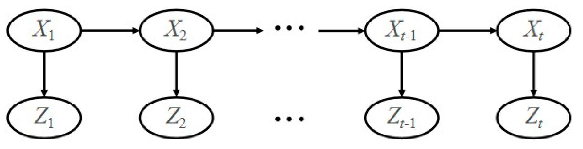
Particle filtering (PF), also known as Sequential Monte Carlo, is a general algorithm for the evolution of state variables in DBNs [30]. Particle filtering approximates probability distributions by sampling a set of random samples and then performs statistical calculations on these samples to obtain the minimum variance estimation of the state; these samples are referred to as “particles”. As the number of particles increases, the probability density function described by all particles gradually approximates the true probability distribution of the state, achieving the effect of optimal Bayesian estimation.

Assume there is a system, as shown in Figure 3, whose state variable X_t∈R^m at time t evolves from the state variable X_t−1∈R^m at time t − 1 according to the following state function:

$${\mathit{X}}_t=f\left({\mathit{X}}_t,{\mathit{v}}_{t-1}\right)$$

(9)

where the vector v_t−1∈R^m represents the noise in the state function.

The observed data Z_t∈R_n can be obtained via the following measurement function:

$${\mathit{Z}}_t=h\left({\mathit{X}}_t,{\mathit{n}}_t\right)$$

(10)

From the perspective of Bayesian theory, the state estimation problem is to calculate the credibility of the current state X_t based on a series of previously available data Z_1:t (posterior knowledge) through recursive calculation. This credibility is the probability formula P(X_t|Z_1:t), which needs to be calculated recursively through prediction and update steps.

The prediction process uses the system model (i.e., state Equation (9)) to predict the prior probability density of the state, which is to guess the future state through existing prior knowledge, that is, P(X(t)|X(t − 1)). The update process uses the latest measurement value to correct the prior probability density and obtain the posterior probability density, which is to correct the previous guess.

It is assumed that the system’s state transition follows a first-order Martov model, that is, the current state X(t) at time t is only related to the previous state X(t − 1). At the same time, it is assumed that the data Z(t) measured at time t are only related to the current state X(t), as shown in measurement equation 10 above.

Assuming that the probability density function P(X_t−1|Z_1:t−1) of time t − 1 is known, the prediction of the probability of the next state X(t) can be written as follows:

$$p({\mathit{X}}_t\left|{\mathit{Z}}_{1:t-1}\right.)={\displaystyle \int p({\mathit{X}}_t\left|{\mathit{X}}_{t-1}\right.)}p({\mathit{X}}_{t-1}\left|{\mathit{Z}}_{1:t-1}\right.)d{X}_{t-1}$$

(11)

where state X(t) is exclusively determined by X(t −1) due to the assumption of first-order Markov processes, i.e., p(X_t|X_t−1, Z_1:t−1) = p(X_t| X_t−1).

After obtaining the new measurement data Z_t at time t, the correction of the prediction of formula 10 based on the measurement data can be stated as follows:

$$p({\mathit{X}}_t\left|{\mathit{Z}}_{1:t}\right.)=\frac{p({\mathit{Z}}_t\left|{\mathit{X}}_t\right.)p({\mathit{X}}_t\left|{\mathit{Z}}_{1:t-1}\right.)}{p({\mathit{Z}}_t\left|{\mathit{Z}}_{1:t-1}\right.)}$$

(12)

where $p({\mathit{Z}}_k\left|{\mathit{Z}}_{1:k-1}\right.)={\displaystyle \int p({\mathit{Z}}_k\left|{\mathit{X}}_k\right.)}p({\mathit{X}}_k\left|{\mathit{Z}}_{1:k-1}\right.)d{X}_t$. The filtering update is now complete.

For generic nonlinear and non-Gaussian systems, it is challenging to arrive at the analytical solution of the posterior probability because the derivation above involves integration for continuous variables. Monte Carlo sampling must be used to address this issue.

2.3.2. Monte Carlo Sampling

The goal of Monte Carlo sampling is to sample the target probability distribution and calculate the target’s expected value. When the number of samples N is large enough, the above formula approximates the true probability of winning. The Monte Carlo method is a mathematical method for calculating the odds of multiple possible outcomes occurring in an uncertain process through repeated random sampling.

$$E\left(f\left({\mathit{X}}_N\right)\right)\approx \frac{1}{N}{\displaystyle \sum _{i=1}^N{\displaystyle \int f\left({\mathit{X}}_N\right)\delta \left({\mathit{X}}_N-{\mathit{X}}_N^i\right)}}d{X}_N$$

(13)

2.3.3. Sequential Importance Sampling

The most basic particle filtering algorithm for sampling in posterior probability distribution is Sequential Importance Sampling (SIS) [31]. Assuming that N samples can be sampled from the posterior probability, the calculation of posterior probability can be represented as follows:

$$P({\mathit{X}}_t\left|{\mathit{Z}}_{1:t}\right.)=\frac{1}{N}{\displaystyle \sum _{i=1}^N{w}_t^i\delta \left({\mathit{X}}_t-{\mathit{X}}_t^i\right)}$$

(14)

where δ is the Dirac function. $w_t^i$ is the weight of the particle.

In other words, the new state ${\mathit{X}}_t^i$ of the ith particle at the time step t is sampled from the distribution with the current state and the observed value Z_1:t as parameters.

At time step t, the weight $w_t^i$ is updated from $w_{t-1}^i$ to the following:

$$w_t^i\propto w_{t-1}^i\frac{\mathrm{P}\left({\mathit{Z}}_t\left|{\mathit{X}}_t^i\right.\right)\mathrm{P}\left({\mathit{X}}_t^i\left|{\mathit{X}}_{t-1}^i\right.\right)}{q\left({\mathit{X}}_t^i\left|{\mathit{X}}_{t-1}^i,\right.{\mathit{Z}}_t\right)}$$

(15)

The SIS algorithm has a problem where the variance in the weights w increases with multiple iterations, and it is even possible for one weight to approach 1 while the others tend toward 0, a phenomenon known as particle degeneracy. This leads to a substantial waste of computational time on the majority of particles with excessively small weights. An effective method to mitigate particle degeneracy is through resampling [32], which involves randomly replicating particles with higher weights and eliminating those with lower weights, thereby focusing the computation as much as possible on particles that have a greater impact on the posterior probability density. In addition, the initial state ${\mathit{X}}_0^i$ is sampled from the joint prior distribution of the state variables, and the initial weight $w_0^i$ of each particle is 1/N. The pseudocode for the standard particle filter algorithm flow is as follows:

(1)

Particle set initialization, T = 0:

For i = 1, 2, …, N. Generate sampling particle ${\left\{x_0^i\right\}}_{i=1}^N$ from prior p(x₀).

(2)

For T = 1, 2, …, t. Cycle through the following steps:

①

Importance sampling for i = 1, 2, …, N. The sampling particle ${\left\{x_t^i\right\}}_{i=1}^N$ is generated from the importance probability density; the particle weight $w_t^i$ is calculated and normalized.

②

Resample: Resample the particle set $\left\{x_t^i,w_t^i\right\}$. The resampled particle set is $\left\{{\tilde{x}}_t^i,1/N\right\}$. The conversion weight ${\tilde{w}}_t$ is recorded as ${\displaystyle \sum _{i=1}^N{\tilde{w}}_t^i{x}_t^i}={\displaystyle \sum _{i=1}^N{\tilde{x}}_t^i}$.

③

Output: calculate the state estimation value at time t,${\widehat{x}}_t={\displaystyle \sum _{i=1}^N{\tilde{x}}_t^i}$.

The process of multiple resamplings tends to replicate particles with higher weights excessively, culminating in a final collection largely made up of identical particles. Such a reduction in the diversity of particles can lead to diminished predictive accuracy, a scenario referred to as particle impoverishment. The conventional approach to mitigate this involves augmenting the initial pool of particles and incorporating new particles throughout the filtering process. However, an increase in the initial particle count significantly escalates computational load, adversely affecting time efficiency. Additionally, the indiscriminate introduction of new particles can infuse the model with fresh uncertainties, impairing its convergence. To address these issues, this study introduces an adaptive strategy for the inclusion of new particles. This strategy leverages the Monte Carlo method to intersperse new particles in every filtering iteration, thereby preserving the diversity of the particle ensemble.

2.4. Dynamic Bayesian Network for Fatigue Crack Growth

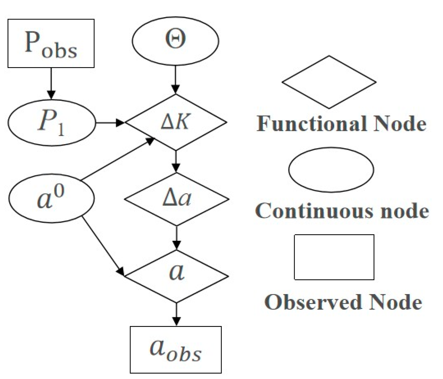
Figure 4 shows the structure of a Bayesian network for one time step. The nodes in the figure are all random nodes, indicating that the variable is random given the value of the parent node; therefore, the arrow pointing to it represents the conditional probability distribution (CPD). The variable names and value ranges of the node symbols in Figure 4 are shown in

Table 1. Bayesian network node variables.

Value	Parameter
Θ	Crack propagation parameters Θ
Δa	Crack increment
Δσ	Equivalent stress amplitude
P	Real load
Pobs	Observed load
a	Real crack length
a0	Crack length before current time step
aobs	Observed crack length
F	Crack shape factor

. Diamond nodes are function nodes, which means that the variable is a deterministic formula calculation result given the value of the parent node; therefore, the arrow pointing to it represents a deterministic function. In addition, elliptical nodes represent continuous variables. Rectangular nodes represent observed variables (such as load and crack length), where Θ refers to all uncertain material fatigue parameter variables considered in the crack propagation formula.

For ease of calculation, all uncertain factors above, except for the initial prior values of fracture toughness, tensile strength, and damage initiation displacement, are assumed to be normal distribution continuous nodes. Usually, load P and crack length a are observable nodes.

2.5. Particle Filter (PF) Equation for Crack Propagation

2.5.1. PF State Equation

The final predicted residual life in the crack propagation model is obtained by the cyclic time at which the crack with initial length a₀ reaches the critical length a_c, which can be regarded as a function of a. Therefore, the goal of particle filtering is to correct the theoretical value of the accumulated crack length output by the crack propagation formula with experimental data a_obs. The estimated crack length in the model is the theoretical length obtained by the crack propagation formula, and Θ refers to all parameters of the crack propagation formula. The process error is denoted as v_a, which is zero-mean Gaussian noise from model error. The formula for the state equation can be expressed as follows:

$$a_t=f\left(\Theta \right)+v_a$$

(16)

This error v_a is added after each theoretical crack length at output by the crack propagation formula.

2.5.2. PF Measurement Equation

The uncertainty of crack observation data depends on the instrument error of the crack observation and the influence of the simplified conversion of irregular crack shape. It is assumed that the measurement error is zero-mean Gaussian white noise, that is, ${\epsilon }_a~N\left(0,{\sigma }_a^2\right)$. The observation data can also be written as $a_{obs}=a+N\left(0,{\sigma }_a^2\right)$, which can prove the following:

$$p\left(a_{obs}\left|a\right.\right)=p\left(a\left|a_{obs}\right.\right)=\frac{1}{{\sigma }_a\sqrt{2\pi }}\exp \left(-\frac{{\left(a-a_{obs}\right)}^2}{2{\sigma }_a^2}\right)$$

(17)

Equation (17) is equivalent to

$$p\left(a_{obs}\left|a\right.\right)p\left(a\right)\propto p\left(a\left|a_{obs}\right.\right)$$

(18)

Among them, a is the real length of the crack, which is an unknown value. This error is included in the crack measurement data, that is, the real length of the crack $a=a_{obs}-{\epsilon }_a$.

ε_a is the measurement error of the crack observation data, which reflects the error between the true value and the measured value of the crack. v_a is the model error of the crack propagation formula, which reflects the error between the true value and the simulated value of the crack. Particle filtering selects whether to rely more on measurement data or model data based on their magnitude.

The crack length data are obtained from fiber optic data and experimental annotations, which brings two sources of uncertainty: measurement error and data sparsity. Similar to the uncertainty of the load, the measurement error in the crack length data depends on the accuracy of the annotation and the processing of the non-uniform crack equivalent length on the layered surface, usually assumed to have a zero-mean Gaussian distribution ${\epsilon }_a~N\left(0,{\sigma }_a^2\right)$. This method can also handle other measurement error distributions. Since crack observation requires manual collection by instruments, crack length data are rarely applicable for every time step. Even if a data point is obtained after each observation and applied to the DBN for diagnosis and prediction, data sparsity introduces data uncertainty.

2.6. Adaptive Particle Filter Correction Method Based on DBN Reasoning

In traditional filtering processes, state equations are often invariant. However, when there is a substantial error between the state equation and the actual state, the predictive accuracy and convergence speed of the filtering may not be ideal. This difference becomes minimal with continuous experimental data input, but in the absence of such data, predictions still exhibit a certain level of deviation. This deviation is particularly noticeable when experimental data are scarce. Additionally, traditional filtering fails to derive correction coefficients for the theoretical formulas associated with the filtering outcomes. To ensure the state equation is continuously updated during the filtering process, it is essential to adjust the parameters of the state equation using the filtering results from each time step. Moreover, to overcome the issue of particle depletion seen in traditional particle filtering, an adaptive sampling approach is introduced.

Assuming the use of Paris’ law, the specific state evolution Equation (9) and observation Equation (10) in Section 2.3.1’s particle filtering formula can be respectively represented as follows:

$$a_t=a_{t-1}+C{\left(\Delta K\right)}^m\cdot \Delta N+v_a^t$$

(19)

$$a_t^{obs}=a_t+{\epsilon }_a^t$$

(20)

where $a_t$ represents the calculated crack length at time t, and $a_t^{obs}$ is the observed crack length at number of cycles t. $v_a^t$ and ${\epsilon }_a^t$ denote the model error and measurement error at number of cycles t, respectively.

Then, through the SIS sampling and resampling described in Section 2.3.3, we can obtain the posterior estimate of the crack length at number of cycles t as ${\widehat{a}}_t={\displaystyle \sum _{i=1}^N{\tilde{w}}_t^i{a}_t^i}$, where $a_t^i$ represents the sample values from particle filtering and ${\tilde{w}}_t^i$ denotes the resample weights of the samples. Similarly, we can obtain the posterior estimate of the parameter ${\widehat{\Theta }}_t$ as ${\widehat{\Theta }}_t={\displaystyle \sum _{i=1}^N{\tilde{w}}_t^i{\Theta }_t^i}$, where ${\Theta }_t^i$ is the parameter corresponding to the particle filtering crack length samples $a_t^i$.

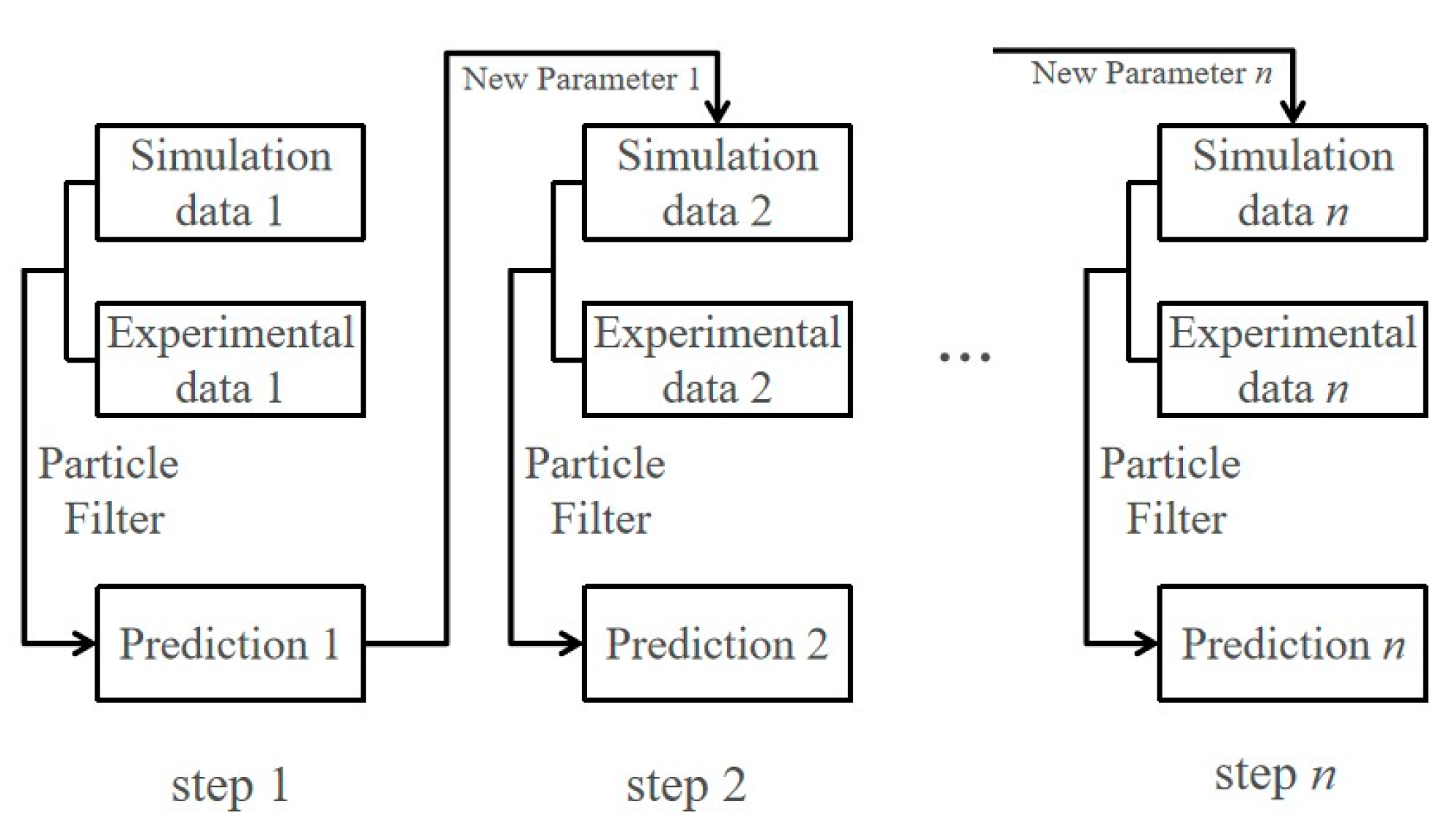
Utilizing the kernel density estimation approach enables us to derive the probability distributions of the posterior estimates for ${\widehat{a}}_t$ and ${\widehat{\Theta }}_t$, thus facilitating the DBN model’s update. Following this, the refreshed posterior parameters ${\widehat{\Theta }}_t$ will act as the preceding parameters ${\Theta }_{t+1}$ for the forthcoming DBN filtering stage in the crack propagation equation. In accordance with their probability distribution, new samples for the time t + 1 are recreated using the Monte Carlo method, paving the way for subsequent updates to the model.

f(·) represents the crack propagation formula. The whole process is shown in Figure 5:

2.7. DBN Whole Frame

This paper proposes an adaptive DBN particle filter, which uses a crack propagation formula as the system state equation of particle filtering and uses material parameters, observed cracks, and loads as input continuous node random variables. The steps of the DBN can be represented as follows:

Step 1. Through the examination of accessible materials (for instance, simulations of identical structures or fatigue expansion formulas), extensive prior data on lifespan under diverse conditions of load, stress ratio, and fracture toughness among other parameters are acquired. These data act as the preliminary parameters Θ₀ for the crack propagation equation. Subsequently, initial particles are generated from the prior probability distribution P(Θ) associated with these parameters by employing the Monte Carlo method, which initiates the values for each node within the DBN.

Step 2. Once the monitoring of crack propagation in structures commences, the equivalent stress Δσ at the crack tip is determined from the observed load $P_{obs}^t$. This value, together with additional prior parameters Θ^t, is incorporated into the crack propagation equation to derive the theoretical crack length at present, $a_t$. Subsequently, this theoretical figure and the observed experimental data also serve as the basis for the state and measurement equations in particle filtering. Employing the adaptive particle filtering technique outlined in Section 2.6, particle filtering facilitates the acquisition of the posterior estimates for the current crack extension length ${\widehat{a}}_t$ and the parameters ${\widehat{\Theta }}_t$.

Step 3. Following the acquisition of posterior parameter samples ${\widehat{\Theta }}_t$ at moment t, the probability distribution of ${\widehat{\Theta }}_t$ undergoes sampling via kernel density estimation. This process inputs the derived samples into crack propagation, serving as the prior update for the crack length particles at the forthcoming moment t + 1. This step facilitates the retrieval of the next posterior filtering values $a_{t+1}$.

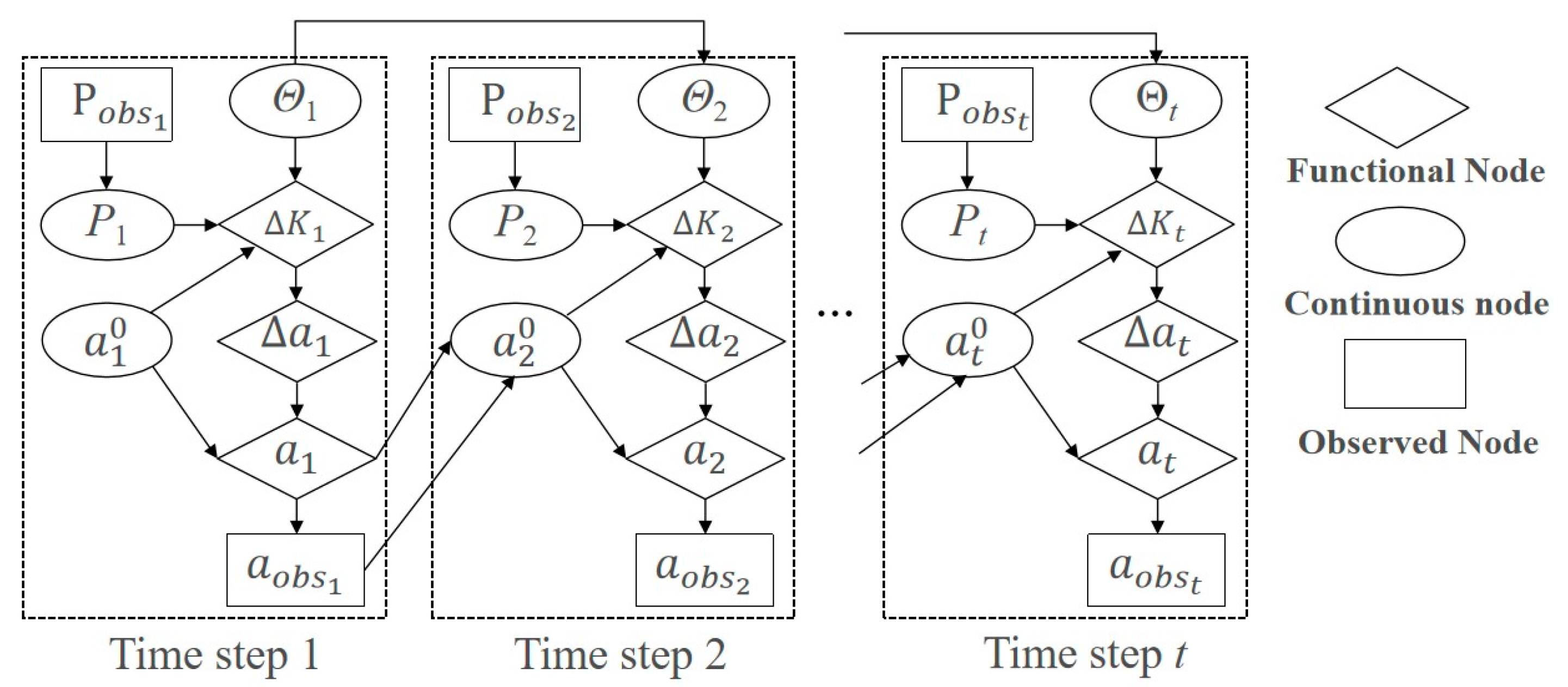
The structure of the overall DBN is shown in Figure 6. The uncertainties mentioned above in the DBN are represented by the nodes in the figure. Nodes are connected by arrows representing conditional probability distributions or deterministic functional relationships. The subscript t − 1 or t represents the time step.

In this section, the DBN model for crack propagation is validated using both single and multiple adaptive variable datasets. Section 3.1 describes the DBN model for crack propagation with a single adaptive variable. In contrast, Section 3.2 presents the DBN model for crack propagation incorporating multiple adaptive variables.

3. Fatigue Crack Propagation Experiment Verification

3.1. Single Adaptive Variable DBN Model

To validate the feasibility of the proposed method, three-point bending fatigue experiments were conducted using three specimens, as shown in Figure 7a. The dimensions of the specimens are 120 × 30 × 15 mm³, 160 × 40 × 15 mm³, and 240 × 60 × 15 mm³, with the support span S being L-0.4×W. The material of the specimens is AL6061 aluminum alloy, with an elastic modulus, E, and Poisson’s ratio, v, of 69.6 GPa and 0.33, respectively. The bending fatigue limit of the material is around 100 MPa. The initial crack length, a₀, is 10 mm, where the length of the prefabricated notch is 9 mm, and the crack length initiated by cyclic loadings, according to ASTM E1820, is 1 mm. According to ASTM E399 standards [33], the material’s fracture toughness K_IC was measured to be 34 MPa. The stress ratio R is 0.2, with maximum loads of 4500 N, 6000 N, and 9000 N. The load magnitudes make the maximum stresses at the lower sides of the specimens (without considering the crack) nearly equal (around 54 MPa).

3.1.1. Data Analysis

The crack propagation a-N curves [34] for the three specimens are shown in Figure 8. According to ASTM E399, the stress intensity factor, K, for three-point bending specimens is calculated using

$$K=\frac{3PS}{2B{W}^2}\sqrt{a}\frac{1.99-\xi \left(1-\xi \right)\left(2.15-3.93\xi +2.7{\xi }^2\right)}{\left(1+2\xi \right){\left(1-\xi \right)}^{\frac{3}{2}}}$$

(21)

where ξ = a/W with a as the crack length; P is the load amplitude. Letting K = K_IC, the critical crack lengths, a_C, of the three specimens were calculated as 20.6, 26.2, and 36.3 mm, respectively. And the measured values of a_C are 20.5, 25.9, and 36 mm. It can be seen that the measured critical crack lengths in Figure 8 are highly consistent with those calculated theoretically.

In addition, fractographs were taken of the fracture sections of the three specimens and are shown in Figure 9a–c. The areas indicating the stages of steady crack propagation and sudden specimen fracture can be well distinguished from the figures, and the regions with the distance of a_c from the lower edge of the specimens exactly locate the transition between these two stages.

Paris’ law was used as the state equation for particle filtering. Based on the experimental data, the parameters of Paris’ law were obtained based on data fitting. Specifically, the value of m in Paris’ law is approximately 3.34, and C ranges from 5 × 10⁻¹¹ to 7 × 10⁻¹¹. Within the context of the DBN, the logarithmic of parameter C is treated as a variable subject to uncertainty. For particle filtering purposes, it is initially represented by a set of uniformly distributed particles. These particles are then subject to passive, adaptive updates in sync with the revisions of the DBN model. To verify the correction ability of the method, observation was started after several cycles and DBN tracking instead of starting from scratch.

3.1.2. Uncertainty Sources Considerations

In the DBN, the error analysis of crack propagation is focused on two primary aspects: model errors and measurement errors. The model errors, particularly those arising from the limitations of Paris’ law, are identified as the core of the analysis. This includes the intrinsic limitations of the formula and the effects of structural defects on the accuracy of material parameter estimations and equivalent stress calculations, which together lead to deviations in performance evaluation. The measurement errors, such as noise from measuring instruments, irregularities in crack paths and shapes, and non-standard operations during the loading process, also significantly impact the accuracy of the assessment. To address these challenges, the DBN in this study considers the following main uncertainty factors:

• Equivalent stress at crack tip.

The equivalent stress is obtained from the calculation of alternating load, and there are errors in the selection of stress intensity criteria, structural defects, and load observation noise. According to experience, it is assumed that the variance of this error is within 10%, so the normal distribution of 10% variance is taken in this paper.

2.

The error of the parameter m for Paris’ law.

The parameter m in Paris’ law is influenced by geometric defects in the structure and material properties, leading to significant variability even within the same material and structure [35]. Therefore, in this study, based on the variability observed in experiments, the initial values of several specimens were averaged and subjected to a Gaussian distribution [36]. Subsequently, after applying filtering and DBN inference, the distribution range of the modified samples was determined through kernel density estimation.

3.

Uncertainty of crack length.

The length of the crack mainly exists in the measurement error of the crack increment in the experiment and the numerical calculation error caused by the non-uniform crack length on the left and right sides as well as the internal crack length. This error is fitted to the binary curve in line with its own trend according to the data, and the fitting variance of the measured data points is taken as 4.6% [37].

The parameter m, serving as a parameter variable within the DBN, undergoes adaptive updates following each round of filtering, whereas other uncertain elements remain unchanged, manifesting merely as errors within the particle filtering process. An initial measurement error is presumed to be 10%. Due to the incremental growth of the crack per cycle being considerably minor in comparison to the initial crack, each subsequent crack increment incorporates an additional 5% measurement error and system process error.

3.1.3. Model Results and Data Graphs

The first 90% of the cycle times are taken as the observation data of this method, and the last 10% are taken as the verification of accuracy. The change in the uncertainty parameters obtained according to DBN reasoning after filtering is shown in Figure 10. The notation “log(·)” denotes an operation using the natural logarithm.

As can be observed from Figure 10, the uncertainty range of parameter C is quickly narrowed after the first filtering. This demonstrates the efficacy of the DBN in facilitating node adjustment. With the model being updated step by step, the uncertainty range of C steadily decreased, converging after approximately 4–5 iterations. The updated value was very close to the measured data.

The final crack propagation prediction of the DBN particle filter is shown in Figure 11. Due to the scarcity of crack observation data, if there is no observation value in the current time step, the prediction value will be used instead.

As shown in Figure 11 and Figure 12, due to the lack of observational data, the fatigue crack growth and remaining life were significantly underestimated in the first 2–3 filtering processes, with prediction errors reaching as high as 20% to 30%. With the continuous collection of observational data, the uncertainty in the DBN was updated, thereby gradually improving the prediction accuracy. Especially when the filtering process exceeded six iterations, the prediction error for the residual life of specimens could be maintained below 5%, which has practical implications for the safety assessment and maintenance of structures.

3.2. Multiple Adaptive Variables DBN Model

To provide additional evidence regarding the effectiveness of the DBN particle filter, experiments from Zheng [38] were utilized to continue the validation process.

The single-edge crack growth test material is domestically sourced commercial galvanized high-strength steel wire, with a diameter of 7 mm.

For finite-width, equal-thickness strip specimens with unilateral cracks, the calculation formula for the crack form factor F can be obtained from the Stress Intensity Factor Manual, as shown below:

$$F=1.12-0.234\left(\frac{a}{b}\right)+10.55{\left(\frac{a}{b}\right)}^2-21.72{\left(\frac{a}{b}\right)}^3+30.39{\left(\frac{a}{b}\right)}^4$$

(22)

where a is the crack length and b is the specimen width.

Zheng adopts the Walker law as the prediction formula for crack propagation [27].

$$\frac{da}{dN}=C{\left[{\left(1-R\right)}^{\alpha }\Delta K\right]}^m$$

(23)

The experiment collected separate data on crack propagation at stress ratios R = 0.1, R = 0.5, and R = 0.7. The parameter m of Paris’ law is 3.3. The crack propagation data under a 220 MPa load were utilized as the validation dataset for the DBN model, as depicted in Figure 13. The author performed a parameter fitting process to determine the values of parameters C and α; the obtained values were approximately 7 × 10⁻¹³ and −0.3, respectively, with a survival rate of 95%.

The parameters in

Table 2. DBN uncertain variables.

Parameters	Initial Value	Standard Deviation	Meaning
Log(C)	−27	1	The logarithm of parameter C
α	−0.3	0.01	Stress ratio coefficient
a0	0.001	0.0001	Prefabricated crack error (mm)
aobs	0.001	0.0001	Measurement error εa

are utilized as sources of uncertainty for the DBN particle filter. The parameters C and m are adaptively updated in the DBN model update. The mean and variance of sampling for other uncertain variables remain unchanged.

The prediction results of the DBN particle filter are shown in Figure 14.

Figure 15 demonstrates that the adaptive DBN model is equally capable of accurately forecasting the actual progression of crack expansion across varying stress ratios. In comparison to the three-point bend model examined in Section 3.1, there are less observational data available for this section’s single-edge crack model. Additionally, the uncertain variable parameter Θ within the Walker law is not linear but includes a power exponent variable, which magnifies the errors. When utilizing the initial model to predict crack expansion reliability, the overlapping uncertainties of various model parameters Θ lead to a wider range of predicted crack intervals. This range only narrows, adopting a “trumpet” shape, after incorporating the next batch of observational data, which prompt an update in the model’s state. Following this update, the precision of crack predictions improves, and the uncertainty interval diminishes, demonstrating that the update enables the particles to more closely mimic the true probability distribution between two observational points. As predictions advance, the estimates increasingly diverge from the actual conditions, and the uncertainty interval expands accordingly. This expansion results from the model’s uncertainty propagation, which continually escalates the prediction errors, highlighting the importance of ongoing crack monitoring and frequent updates to the model’s state.

Figure 16 and Figure 17 showcase the variations in the probability distribution of Walker model parameters.

As depicted in Figure 16, the values of C predicted by the DBN and given in [38] are slightly different, where the predicted values are lower at R = 0.5 and 0.7 and higher at R = 0.1. This is because the C value in [38] was averaged among three experiments with different stress ratios, whereas the predicted values based on the DBN are obtained based on each individual experiment. The deviation in C is mainly attributed to the dispersion in material properties. In general, the average of the predicted values is consistent with that in [38]. For α, the predicted value is basically consistent with that in [38], as can be seen in Figure 17.

4. Discussion

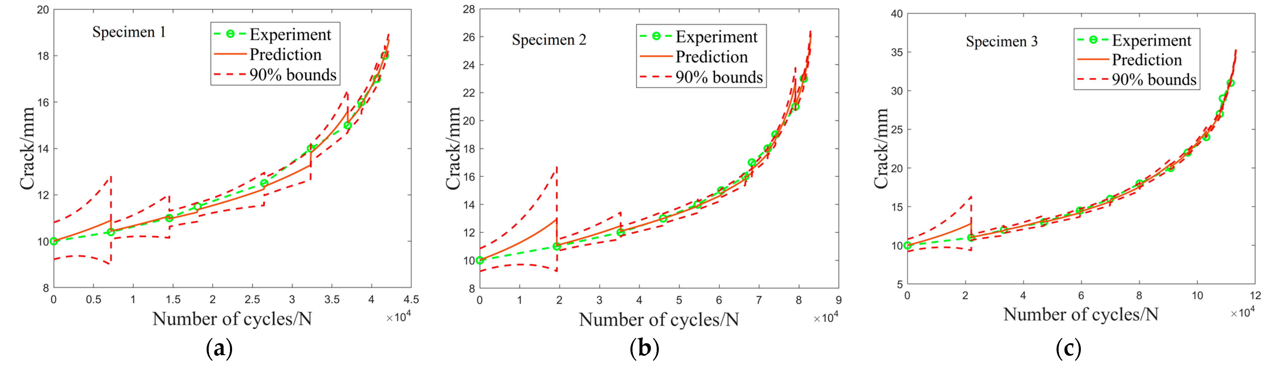
This paper presents a crack propagation prediction model using a DBN, suitable for effective tracking of damage evolution in aerospace structures. The method is validated using experimental data from three-point bending and single-edge crack tension tests. 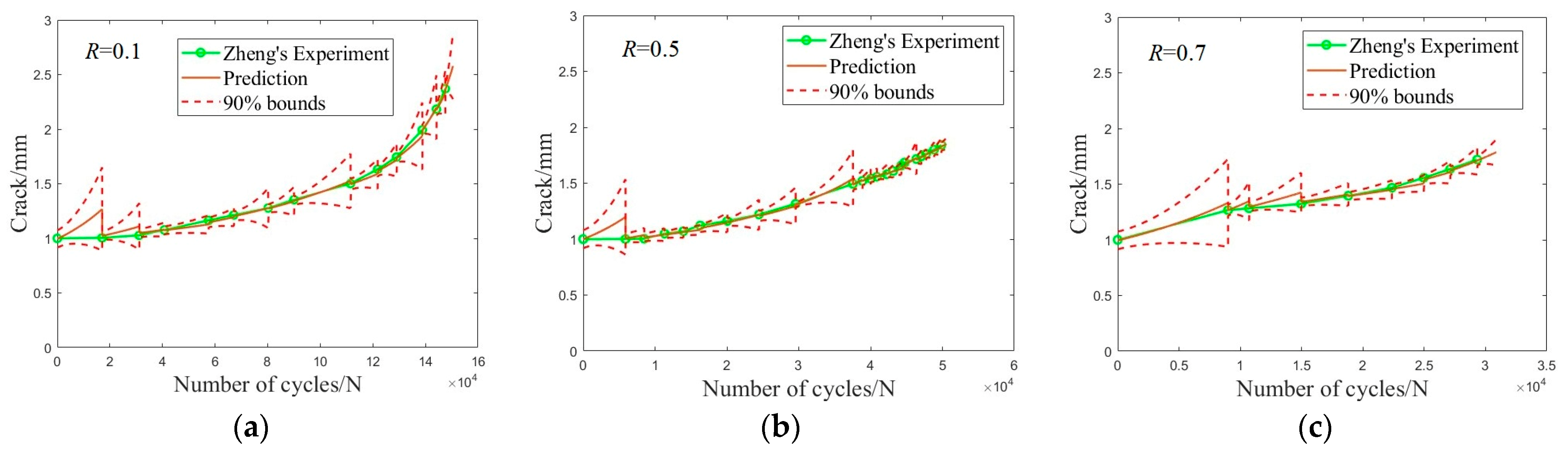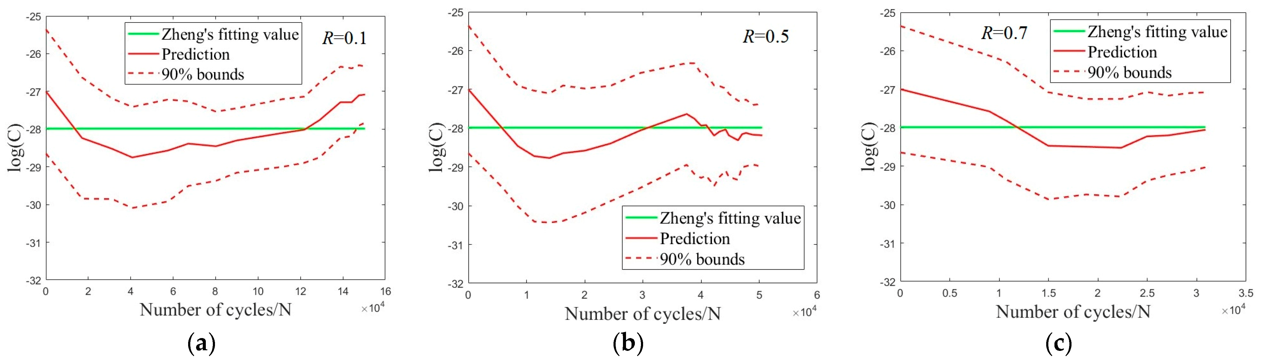The results show that through DBN particle filtering, the uncertainty interval for crack propagation in the three-point bending specimen decreased from 24% to 6%, as shown in Figure 11, and the prediction error for the lifespan was also reduced from over 30% to lower than 5%, as shown in Figure 12. In the single-edge crack experiment, although multi-source uncertain variables increased the uncertainty interval of crack propagation, the error range of the filtered uncertainty interval gradually decreased, and the prediction error for the uncertain variables, Θ, also exhibited the trend of gradual decrease and convergence. This indicates that the DBN filtering can track and correct time-dependent variables (crack length) and reduce the uncertainty of time-independent variables (parameter Θ).

By comparing the single adaptive variables and multiple adaptive variables in the two examples, it is evident that the convergence of the variables in particle filtering decreases along with the enlarged dimension of the uncertain variable space. One potential reason for this is that the interdependence and nonlinear effects among parameters increase the complexity of the system. With multiple parameters involved, the update of each parameter depends not only on its own observed data but may also be influenced by the states of other parameters. This leads to multiple possible solutions within the parameter space. A possible solution includes the improvement method of marginalizing some uncertain variables (such as the Rao-Blackwellized particle filtering method), which is a direction for future research.

As the model is continuously updated, both the parameter variables and the predicted cracks will gradually converge. However, when new uncertainties suddenly emerge, causing significant changes in the prediction outcomes, the variation in parameter means and uncertainty intervals will increase sharply until the new factors stabilize. Subsequently, the uncertainty interval gradually decreases to a new state of convergence.

5. Conclusions

This study introduces a probabilistic approach for health diagnosis and prognosis through an adaptive DBN framework. This framework employs DBNs to predict health conditions and is characterized by its capability to adaptively update parameter probability distributions and regenerate new particle samples, while integrating various sources of inference and cognitive uncertainty. It is suitable for structural health diagnosis and fatigue crack growth prediction under uncertain conditions. The particle filtering algorithm is utilized within the DBN for Bayesian inference to calibrate the physical model. The proposed method has been validated through two experimental data examples, confirming its advantages: (1) It can track the evolution of time-related state variables and reduce uncertainty variables in time-independent states (diagnosis). (2) It allows for the self-calibration of parameter probability distributions and prediction structures through real-time updates, forecasting fatigue crack growth and residual life probabilistically (prognosis), demonstrating excellent stability and robustness. (3) Adaptive updating and regeneration of particles prevent particle depletion, rendering the model’s outcomes more realistic compared to traditional particle filtering results.

In addition, the current model also has some limitations for future enhancement. Firstly, the model’s capability is limited to tracking single crack damage, overlooking the interaction and combined effects of multiple crack damages. Secondly, the experimental scenarios used in the model are relatively simple. In contrast, the operational environment of aerospace structures is evidently more complex, posing challenges for accurate simulation and prediction.