The Remaining Life Prediction of Rails Based on Convolutional Bi-Directional Long and Short-Term Memory Neural Network with Residual Self-Attention Mechanism

Abstract

In the railway industry, the rail is the basic load-bearing structure of railway tracks. The prediction of the remaining useful life (RUL) for rails is important to avoid unexpected system failures and reduce the cost of maintaining the system. However, the existing detection of rail flaws is difficult, the rail deterioration mechanisms are diverse, and the traditional data-driven methods have insufficient feature extraction. This causes low prediction accuracy. With objectives set in relation to the problems outlined above, a rail RUL prediction approach based on a convolutional bidirectional long- and short-term memory neural network with a residual self-attention (CNNBiLSTM-RSA) mechanism is designed. Firstly, the pre-processed vibration data are taken as the input for the convolutional bi-directional long- and short-term memory neural network (CNNBiLSTM) to extract the forward and backward dependencies and features of the rail data. Secondly, the RSA mechanism is introduced in order to obtain the contributions of the features at different moments during the degradation process of the rail. Finally, an end-to-end RUL prediction implementation based on the convolutional bi-directional long- and short-term memory neural network with the residual self-attention mechanism is established. The experiments were carried out using the full life-cycle data of rails collected at the railway site. The results show that the method achieves a higher accuracy in the RUL prediction of rails.

1. Introduction

Because of the significant capacity, high efficiency, energy consumption, and low transport costs of heavy rail transport, it is both widely used and valued in different countries across the world. Rail transport has been internationally recognized as the direction of development for bulk cargo transport, especially in China due to its vast, uneven distribution of resources across the country [1,2]. However, with the increase in train speeds and railway capacity, railway defects and even failures occur frequently. The type of railway section fault in mountainous areas has also changed from the previous type of rail fault—which is based on the side grinding of the upper strand of the curve, the thick edge of the lower strand, and the abrasion of the rail on the long gradient—to the rail defect—which is based on stripping off the blocks, cracks, and abrasions. The rail is an essential part of the line equipment, directly bearing the rolling stock load, so the service state of the rail directly affects the operational state of the heavy railway. Therefore, it is essential for the operation of heavy railways to accurately detect the operating condition of rails and predict their RUL [3].

The RUL of rails is realized via feature extraction, construction of life prediction models, and other techniques based on current or historical inspection data and other information. Therefore, the research focus, when considering RUL, is on how to use data-processing and -mining techniques to construct suitable models and extract typical features from rail data. Residual life prediction models are generally classified as physical model methods, statistical model methods, and data-driven methods [4]. The physical modeling approach assesses the health of a system through the construction of mathematical models based on failure mechanisms or first principles of damage [5]. Li et al. [6] proposed a numerical model based on the simulation of rail profile wear, which, by applying improved models such as Kalker’s non-Hertzian contact, simulated the shape of the worn rail profile in general agreement with the field measurements. Wang et al. [7] developed a numerical model of vehicle track based on the multi-body dynamics and the improved Archard wear formula, and a numerical model of vehicle trajectory was developed to characterize the development of high rail-side wear in a heavily trafficked transport track. This approach is highly descriptive as system degradation modeling relies on natural laws. However, the method suffers from problems, such as high cost and complexity of implementation, and is not readily accepted in engineering practice [8]. The statistical modeling method is based on historical data and statistical learning, which builds a prediction model by fitting and analyzing historical data to predict the RUL. Xu et al. [9] used an inverse Gaussian (IG) stochastic process to establish a structural resistance degradation model, which was updated in real time using the Bayesian updating theory and demonstrated the feasibility of the method with numerical examples. Due to the irregularity of the track structure damage, it is very difficult to establish the exact mathematical statistics in practical applications, and the dynamic characteristics of the machine cannot be taken into account.

In recent years, neural network methods, like convolutional neural networks (CNNs) [10,11] and recurrent neural networks (RNNs), have become the most commonly used data-driven-based methods [12]. By extracting features, they reveal potential correlations and causal relationships between the collected data and the health state of the machinery and provide an end-to-end solution for solving the RUL prediction problem [13]. Therefore, these data-driven approaches have gradually become mainstream in recent years. The long short-term memory network (long short-term memory, LSTM) [14] and its variants have all been successfully adapted to the field of RUL prediction in succession. Ma et al. [15] introduced a deep neural network based on a convolutional long short-term memory (CLSTM) network, which contains the time-frequency information as well as the temporal information of the signal. This network retains the advantages of LSTM and incorporates time-frequency features to accurately predict RUL. However, the LSTM only predicts future data by capturing past data. Bi-directional long short-term memory (BiLSTM) simultaneously acquires future and past information, demonstrating better qualities in RUL prediction [16]. Zhao et al. [17] used a BiLSTM neural network to learn intrinsic features in both directions and improved the fault recognition accuracy. Li et al. [18] proposed a multi-branch improved convolutional network (MBCNN)-BiLSTM model for predicting bearing RUL. MBCNN achieves spatial feature extraction of orientation input data, and then BiLSTM further mines the temporal features of the data, thus improving the prediction accuracy of bearing RUL. Sun et al. [19] proposed a complete ensemble empirical mode decomposition (CEEMD)-CNN-LSTM model, which was experimentally verified to have higher prediction accuracy than single CNN and LSTM. The above study shows that fully extracting data features can improve the prediction performance and achieve better prediction accuracy. Although CNNs and LSTM can extract data features well, they are not fully suitable for rail vibration signals, because CNN is deficient in temporal feature extraction and LSTM is deficient in local feature extraction. In contrast, combining the two can make better use of the advantages of both, thus improving the ability of feature extraction.

Due to the special characteristics of the existing rail inspection, the full life-cycle data of rail injury and damage have the characteristics of low frequency and long time span, and at the same time, it is difficult and costly to explore the failure mechanism of rails involving complex wheel–rail relationship problems. In addition, a series of problems, such as gradient explosion and disappearance, and large memory occupation, have not been properly solved during the process of model training. Meanwhile, if the prediction accuracy is not enough, it may cause significant economic damage and casualties. This poses a challenge to deep learning-based RUL prediction for railway tracks.

In recent years, attention has arguably become one of the most important concepts in the field of deep learning. With the development of deep neural networks, the attention mechanism has been widely used in various application areas [20]. It has been shown that the attention mechanism has better access to the extracted feature information [21]. Mnih et al. [22] proposed an attention mechanism to solve problems such as gradient vanishing and gradient explosion. The method calculates different weights given to different features of the model. Liu et al. [23] proposed an end-to-end RUL prediction method based on feature-attention, which applies the proposed feature-attention mechanism directly to the input data so as to dynamically assign greater weights to more important features during training, thereby improving the prediction performance. The residual connection can enhance the gradient propagation, thus solving the problem of the increase in network depth that can easily cause gradient disappearance and gradient explosion [24]. Xu et al. [25] proposed a CNN-LSTM-Skip model to estimate the State of Health (SOH) of lithium-ion batteries. Jump connections were added to the Convolutional Neural Network–Long Short-Term Memory (CNN-LSTM) model in order to solve the problem of neural network degradation caused by multilayer LSTM. Cao et al. [26] presented a temporal convolutional network–residual self-attention mechanism (TCN-RSA), where the RSA scans through the global information and discovers local useful information, thus achieving the function of enhancing useful information and suppressing redundant information. The above method provides ideas for solving the problem of defects in rail inspection data.

This paper presents a new approach to deriving the RUL of railway rails from the vibration information caused by wave abrasion and other injuries in heavy railways and to construct a feature extraction module, CNN-BiLSTM, which extracts the temporal features of the data and effectively extracts the forward and reverse dependencies of the data without requiring significant familiarity with the failure mechanisms of the rails. This effectively overcomes the limitations of the above literature in performing more comprehensive feature extraction from the data, including the challenge of using expert knowledge to build accurate damage-tracking models. Different attention mechanisms have satisfactory results. However, the self-attention mechanism in the above literature involves a large number of weight matrix operations; the optimization of the weight matrix optimization is usually difficult in traditional deep learning methods, the gradient of the error function must be back-propagated layer by layer, and the error function has a poorer optimization effect or the gradient disappears after back-propagation on the weight matrix. To address this problem, the RSA module is constructed, which solves the above problem by adding the residual self-attention mechanism with residual connection; at the same time, the RSA can also obtain the internal correlation features, which effectively improves the expressive ability of the model. The proposed method is validated and analyzed by experimenting with the vibration data collected by our team in a railway section. The contributions are as follows:

(1)

A CNNBiLSTM-RSA model is proposed to establish an end-to-end prediction model between monitoring the data and the remaining service life of rails by using indirect data such as vibration signals caused by rail damage. A case study of the proposed method is carried out on different types of rail damage and roll bearings, and the CNN-BiLSTM-RSA has a better nature in terms of prediction accuracy, as well as a certain generalization ability.

(2)

The CNN-BiLSTM feature extraction module is constructed to make full use of the advantages of both to enhance the feature extraction capability, which can adaptively extract features and reduce the influence of artificial factors to a certain extent.

The rest of the paper is structured as follows: The framework of the presented prediction method is presented in Section 2, and the individual components are described in detail. Section 3 presents the rail data and details the experimental results and related analyses. Finally, the conclusions are presented in Section 4.

2. RUL Prediction for Rails Based on CNNBiLSTM-RSA

Trains run on and between the track coupling process is complex and variable, thereby giving rise to various types of rail injuries. Among them, stripping, wave abrasion, fish scale, and other defects are the most common, and different types of rail defects have different impacts on line operation. For example, if the stripping length is more than 15 mm and the width is more than 3 mm, it is regarded as a slight defect and needs to be polished. When the stripping reaches a length of 25 mm and a depth of more than 3 mm, it is considered to be a serious defect and requires replacement of the rail [27]. RUL is a predictive maintenance metric used to estimate the remaining time or service life of a component or system before it reaches a critical state or a failure state. In this study, the direct structure of the data-driven approach [28] is adopted for typical injuries and damages to rails. The RUL of a railway track can be directly derived from the vibration information caused by spalling and other injuries during the whole life cycle of heavy railway rails. The method can be applied to the track life prediction of in-service railway tracks. The schematic diagram of the proposed end-to-end prediction model is shown in Figure 1. The prediction model mainly consists of a feature extraction layer, a residual self-attention module, and a fully connected layer.

The original vibration data of the rail are preprocessed as the sample of the model input. The feature extraction module is composed of a combination of CNN and BiLSTM, which effectively combines the feature processing capability of CNN and the temporal association capability of BiLSTM. This allows the model to better extract the vibration signal features from the rail. Meanwhile, to make better use of the extracted timing information, the position encoder in the transformer model is used to encode the position of the features extracted by the CNNBiLSTM model. Then, an RSA mechanism is constructed behind it to obtain the contribution of different moments in the time series. Meanwhile, residual connectivity is introduced into the CNNBiLSTM-RSA network through its feature of transmitting data across layers. This avoids the gradient vanishing problem in the network and enhances the trainability and network expressiveness of the network. Finally, the mapping between the rail features and the RUL labels is established through the fully connected layer.

2.1. Feature Extraction Module

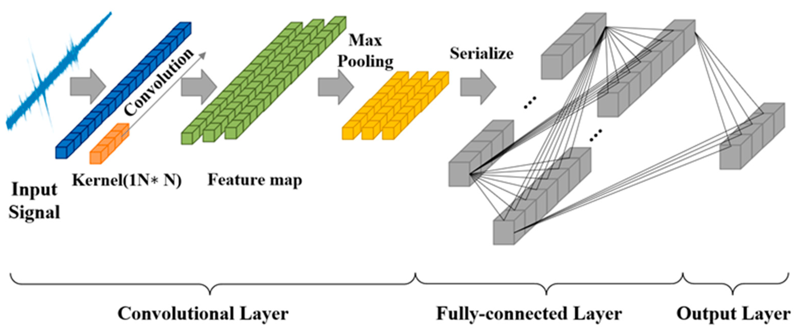
The use of expert knowledge to determine the rail degradation to manage the full life-cycle data of the rail can increase the interference of artificial factors to a certain extent. Allowing the feature extraction module to adaptively learn the fault features without any signal processing to a certain extent can avoid processing the original sample data, thereby reducing the impact of artificial factors. The CNN-BiLSTM module is constructed and includes a convolutional layer, ReLU, MAXpool, and BiLSTM layer. The rail vibration signal belongs to the single-dimensional time series signal, for which 1DCNN is usually used. A typical 1DCNN structure is illustrated in Figure 2. The input vibration signal is expressed as $X=[x_1,x_2,\cdots x_N]$. Features in different regions are extracted by multiple one-dimensional convolution kernels. The convolution operation is defined as follows:

$$X_i=f_i(w^T{x}_{i-1}+b_i),$$

(1)

where $b_i$ and $f_i$ denote the bias term and activation function, respectively. The ReLU function is expressed in the following form:

$$f(X)=\max (0,X).$$

(2)

Then, the features extracted through the convolution calculation are used as inputs for the pooling layer, the sequence is downsized, the network model is simplified by pooling calculation, and the maximum pooling is selected in this paper. A multi-layer convolutional layer and pooling layer are designed. This allows the characteristics of the rail vibration signal to be effectively extracted. Finally, the output of the pooling layer is used as the input for the fully connected layer. However, CNNs have a weak ability to associate features in long sequence information [29].

Although CNN has the ability to automatically extract features from data, it is less capable of handling time-series data with strong time dependence; in contrast, LSTM can effectively solve the long-term dependence problem due to the introduction of gating units. By combining the two, the extraction of spatial and temporal features can be enhanced and the computation time can be relatively reduced. BiLSTM and LSTM are both variants of RNNs (recurrent neural networks), which can effectively avoid the long-term dependency problem caused by gradient vanishing or gradient explosion during the training process of RNN [30]. Compared to the RNN, the LSTM enables the learning of long-term memory through gating units. Many studies have demonstrated that LSTM is effective in dealing with the temporal relationship between inputs and outputs and in learning the data correlation of the time series [31]. LSTM maintains the current recurrent neuron state based on the current inputs and the previous recurrent neuron states. The LSTM unit introduces four gating units defined as the input gate, the output gate, the forgetting gate, and the self-recycling memory unit in order to control the different memory units in their information flow interactions with each other [32]. In the hidden unit, the forgetting gate chooses which state information to keep or forget from previous time steps; the input gate determines what pattern of input vectors needs to be fed into that memory cell state; by comparison, the output gate controls how it changes other memory cell states. It is assumed that $X_t$ and $H_t$ denote sequential input data and cyclic output state at time step t, respectively. The gate, hidden output, and cell state are expressed as follows:

$$\left\{\begin{array}{l}{I}_t=\sigma (U_i{X}_t+W_i{H}_{t-1}+b_i),\hfill \\ F_t=\sigma (U_f{X}_t+W_f{H}_{t-1}+b_f),\hfill \\ O_t=\sigma (U_o{X}_t+W_o{H}_{t-1}+b_o),\hfill \\ \begin{array}{l}{\tilde{C}}_t=\tanh (U_c{X}_t+W_c{H}_{t-1}+b_c),\hfill \\ C_t=F_t\otimes C_{t-1}+I_t\otimes {\tilde{C}}_t,\hfill \\ H_t=O_t\otimes \tanh (C_t),\hfill \end{array}\hfill \end{array}\right.$$

(3)

where U denotes the weight matrix of the respective gate; $W_i$, $W_f$, $W_o$, and $W_c$ denote the corresponding recursive weight matrix of the respective gate.

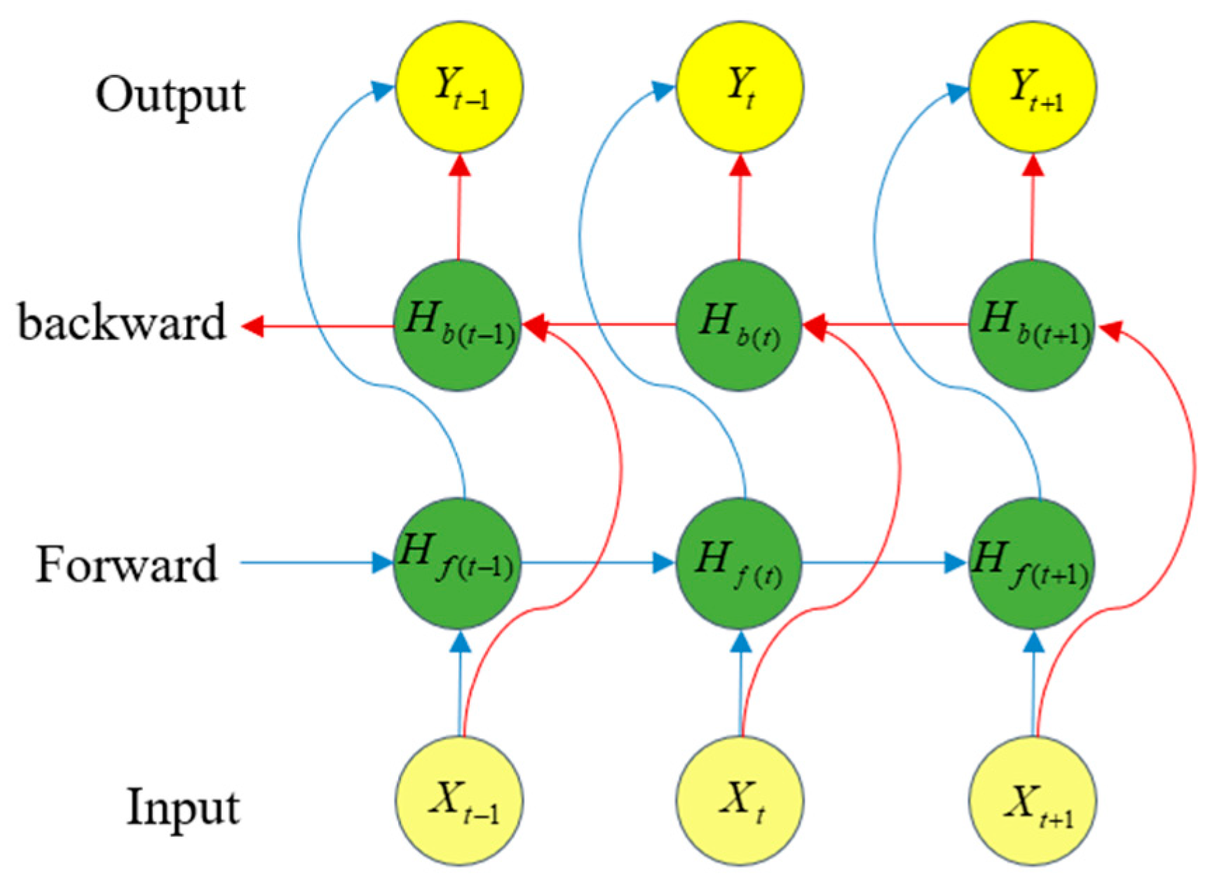
However, LSTM only uses previous information to predict the current state. It cannot use information from a future time. To address this problem, BiLSTM obtains bi-directional information from both historical and future time data and has a more powerful feature learning performance than LSTM. BiLSTM is designed with a bi-directional structure. This structure captures the time series data representations in both forward and backward directions, as shown in Figure 3. BiLSTM superimposes two parallel layers of LSTM in both the forward and backward directions of propagation. The internal state stores information from past time-series values in $H_{f(t)}$ in the forward direction; information from future sequence values is stored in $H_{b(t)}$ in the backward direction. Separate hidden states $H_{f(t)}$ and $H_{b(t)}$ at time step t are sequentially connected to obtain the final output. The recursive states of the BiLSTM are expressed as follows:

$$\begin{array}{l}{H}_{f(t)}=\psi (W_{fh}{X}_t+W_{fhh}{X}_{f(t-1)}+b_{fb}),\\ H_{b(t)}=\psi (W_{bh}{X}_t+W_{bhh}{X}_{b(t+1)}+b_b),\end{array}$$

(4)

The final output vector is obtained using the following equation:

$$Y_t=\sigma (W_{fhy}{H}_{f(t)}+W_{bhy}{H}_{b(t)}+b_y),$$

(5)

where $W_{fhy}$ and $W_{bhy}$ are the forward and backward weights, respectively, and $\sigma$ is the activation function.

2.2. Residual Self-Attention Module

In order to fit the characteristics of low frequency and long time span of the full life-cycle data of rail injury and damage, to enhance the temporal feature information, to retain the long-term dependence, and to enhance the weight of the useful information in order to improve the prediction accuracy of rail RUL, the residual self-attention module is constructed. This module consists of the residual self-attention mechanism that incorporates the residual connection, which can obtain the contribution of temporal information and improve the sensitivity of feature mapping to temporal information. Finally, the predicted value of the rail RUL is obtained by the fully connected layer.

2.2.1. Residual Connections

Due to their ability to transfer information across layers, residual connections are an effective approach for training deep networks. The residual block includes branches that lead to a number of transformations of H as shown in Figure 4. The output of the changes in H and the original output merged are expressed as follows:

$$Y=Activation(X+H(X)),$$

(6)

Typically, the network becomes more expressive and performs better as the number of layers in the network deepens. However, the increase in the number of layers brings problems such as gradient vanishing and gradient explosion. Meanwhile, residual connectivity is very beneficial for very deep networks by allowing the learning layer to modify the identity mapping without performing the entire transformation. Therefore, at the end of the CNNBiLSTM-RSA residual connections are used so as to avoid problems like gradient vanishing and gradient explosion.

2.2.2. Self-Attention Mechanism

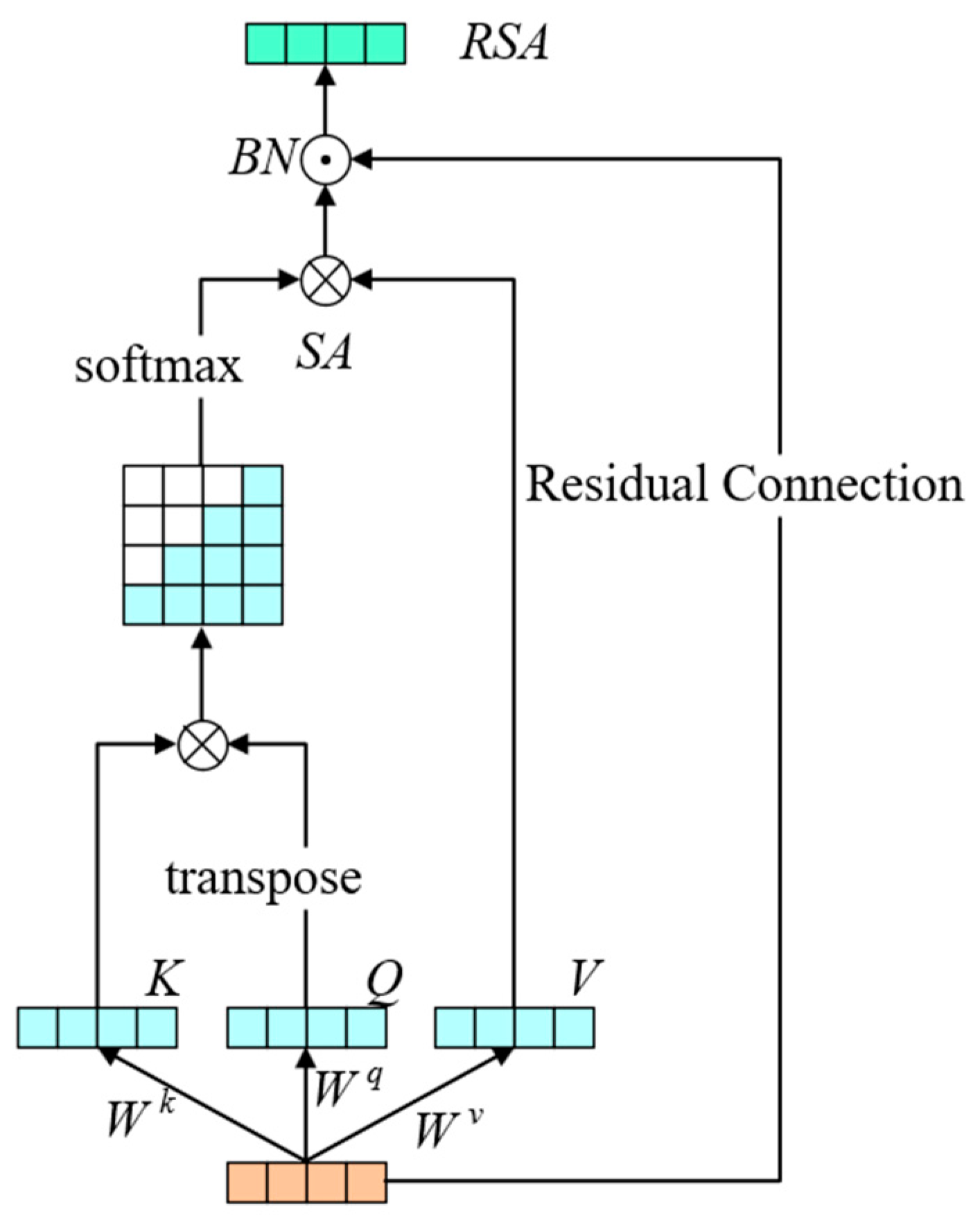
The self-attention (SA) mechanism is the central idea of the transformer model [33]. The SA mechanism allows the model to focus more on the information that contributes more to the output. The RSA mechanism module is improved to capture information with different contributions in the sequences, which improves the expressive ability of the network. This also enables the model to better learn the mapping relationship between the features and RUL labels. As shown in Figure 5, the model calculates the different weights between the elements in the sequence.

The input of the RSA mechanism consists of three parts, which are query (query, Q), key (key, K), and value (value, V) [29]. They are computed using the following equation:

$$\begin{array}{l}Q=W^{q}X,\\ K=W^{k}X,\\ V=W^{v}X,\end{array}$$

(7)

where $W^q$, $W^k$, and $W^v$ are weight matrices.

The value of SA is calculated as follows:

$$SA(Q,K,V)=soft \max (\frac{Q{K}^{\mathrm{T}}}{\sqrt{d_k}})V,$$

(8)

where $d_k$ is the dimension of the key vector; the $soft\max$ function obtains the weight of each value.

Finally, the SA and the inputs are fed through the residual connection into the batch-regression layer to compute the value of the RSA:

$$RSA=BN(SA+input).$$

(9)

In order to better utilize the timing information in the features coming out of the feature extraction module, the position encoder in the transformer model is added to encode the position of this signal feature before the RSA mechanism [34]:

$$\begin{array}{l}P{E}_{(pos,2i)}=\sin (pos/{10000}^{2i/d}),\\ P{E}_{(pos,2i+1)}=\cos (pos/{10000}^{2i/d}),\end{array}$$

(10)

where pos denotes the position number in the sequence; d denotes the dimension of the sensor; 2i denotes an even number of sensors; 2i + 1 denotes an odd number of sensors.

3. Experimental Results and Discussion

3.1. Experimental Data Presentation and Pre-Processing

The data used in the experiment include the whole life-cycle vibration data collected from a railway section, which reflects the state of the rail from normal to degraded up to the point of failure. Sensors with three channels were placed in different positions on the train to acquire vibration signals from horizontal, front–back, and vertical directions. Four working conditions are combined with different train speeds and loads, as shown in

Table 1. Heavy-haul railway rail dataset.

Operating Condition	Running Speed	No-Load		Type of Damage
condition 1	Low speed	unladen	stripping off the blocks (A_1)	Wave abrasion (B_1)	fish scale injury (C_1)
condition 2	Low speed	load	stripping off the blocks (A_2)	Wave abrasion (B_2)	fish scale injury (C_2)
condition 3	high speed	unladen	stripping off the blocks (A_3)	Wave abrasion (B_3)	fish scale injury (C_3)
condition 4	high speed	load	stripping off the blocks (A_4)	Wave abrasion (B_4)	fish scale injury (C_4)

. Under each working condition, there are three different types of rail damage: wave abrasion, fish scale injury, and pieces stripping off the blocks. The actual state of damage to the rail is shown in Figure 6. Because the shape of the rail is different under different types of damage, the corresponding input shapes of the three types of rail damage are wave abrasion, fish scale injury, and stripping off the blocks, respectively. The corresponding input shapes are 3 ∗ 5000, 3 ∗ 3000, and 3 ∗ 2500. The vibration sequence is sampled and recorded as a sample each time the detection train passes through the damaged defects. The data from the three channels of the sensor are stacked under each condition, i.e., horizontal, fore–aft, and vertical vibration signals were used simultaneously. In order to ensure that each experiment is consistent for the training and the test sets, the samples collected during the forward passage of the train are used as the training set for each condition, and the reverse passage is used as the validation and test set. When testing a certain type of damage under a certain working condition, the vibration data of other damage under the same working condition were used for training.

3.2. Experimental Equipment and Experimental Parameter Settings

The experimental environment used in this paper is described as follows.

Hardware environment: (1) 13thGen Intel^®Core^TM i5-13500HX 2.50 GHz (2) 16 GB RAM (3) RTX3080. A 64-bit operating system. The model was implemented in Python 3.10 using Pytorch 2.0.1.

Some appropriate hyperparameters are needed to be selected in the model to ensure the accuracy of the model predictions. Model performance is usually verified using grid search and cross-validation as a means of obtaining the best performance of the model. The k-values of cross-validation may affect their sensitivity to changes in the training set, which in turn affects the hyperparameter selection results; therefore, a grid search for hyperparameter selection has been applied in this paper. The training method used is multi-batch training, the number of samples in each batch is 16, the number of training batches is 100, and the initial learning rate is set to 0.001. In addition, the selected optimizer is Adam. The parameter structure of the model is demonstrated in

Table 2. Model structure parameter settings.

Feature Extraction Module	1DCNN	In_channels= 3
		Out_channels = 32
		kernel_size = 3
		padding = 1
	Max_Pooling	kernel_size = 2
	BILSTM	input_size = 32
		hidden_size = 32
		kernel_size = 2
	Batch Normalization
	Dropout
	Residual connection
	Fully connected
Train	Epoch = 100	batch_size = 16
		optimizers = Adam
		lr = 0.001

.

3.3. Evaluation Metrics

The performance of the presented method is compared with others. The mean absolute error (MAE) [35] and root-mean-square error (RMSE) [36] are selected to evaluate the performance of the methods and are defined as follows:

$$\begin{array}{l}MAE=\frac{1}{n}{\displaystyle \sum _{i=1}^n\left|r_i-{\overline{r}}_i\right|},\\ RMSE=\sqrt{\frac{1}{n}{\displaystyle \sum _{i=1}^n{(r_i-{\overline{r}}_i)}^2}},\end{array}$$

(11)

where $r_i$ and $\overline{r_i}$ are the actual and predicted RUL, respectively.

The vibration data collected in each of the three directions are stacked into one sample and the input data are normalized in the data preprocessing. In this paper, the life percentage of the rail is used as the output label [37], i.e., the actual rail RUL of the rail is normalized to a range of 0–100%. For each sample indexed, the output label is the life percentage of the rail, i.e., the ratio of the current sample indexed value to the total number of full life cycles. That is, when this ratio is 0, the rail reaches full life into failure. The normalized value is calculated as follows:

$$RUL=\frac{f(x)}{T}\ast 100$$

(12)

where f(x) is the true RUL at that time.

With the increase in the number of iterations, the loss function value decreases in the training process and gradually tends to be stable. The experimental results are demonstrated in Figure 7. As shown in Figure 7 the RUL prediction curve is better fitted to the labelled value of the actual RUL. The results preliminarily prove that the presented method effectively predicts the accurate rail RUL.

To further validate the superiority of the model, the prediction results of the model presented in this paper are compared with the CNN, the CNNLSTM network, and the CNNBiLSTM network. The RAE and RMSE values under various operating conditions are shown in Figure 8 and Figure 9.

As seen from the figure, the MAE and RMSE values of the CNNBiLSTM-RSA model are lower than those of the other three algorithms, which shows that the CNNBiLSTM-RSA model has higher prediction accuracy. This is due to the fact that the introduced RSA mechanism avoids the problems of gradient vanishing and gradient explosion that exist in typical recurrent networks.

To verify the effectiveness of RSA in improving model performance through ablation experiments, the models involved in the experiments include CNNBiLSTM networks with an RSA mechanism added to verify the effectiveness and necessity of this mechanism and the combination of CNN-BiLSTM and a traditional SA mechanism to experience the advantages of using the RSA mechanism. The MAE and RSME results of each model in this comparison experiment are shown in

Table 3. Evaluation metrics for ablation experiments under operating condition 1.

Model	Evaluation Metrics		Injury Type
		Wave abrasion	fish scale injury	stripping off the blocks
CNNBiLSTM	MAE	0.0873	0.0947	0.0919
	RMSE	0.1133	0.1230	0.1176
CNNBiLSTM-SA	MAE	0.0566	0.0719	0.0714
	RMSE	0.0797	0.1030	0.0967
CNNBiLSTM-RSA	MAE	0.0456	0.0546	0.0507
	RMSE	0.0647	0.0773	0.0711

,

Table 4. Evaluation metrics for ablation experiments under operating condition 2.

Model	Evaluation Metrics		Injury Type
		Wave abrasion	fish scale injury	stripping off the blocks
CNNBiLSTM	MAE	0.0919	0.0967	0.0939
	RMSE	0.1185	0.1234	0.1247
CNNBiLSTM-SA	MAE	0.0721	0.0851	0.0752
	RMSE	0.0907	0.1254	0.1025
CNNBiLSTM-RSA	MAE	0.0498	0.0615	0.0574
	RMSE	0.0703	0.0849	0.0744

,

Table 5. Evaluation metrics for ablation experiments under operating condition 3.

Model	Evaluation Metrics		Injury Type
		Wave abrasion	fish scale injury	stripping off the blocks
CNNBiLSTM	MAE	0.0900	0.0958	0.0930
	RMSE	0.1173	0.1205	0.1172
CNNBiLSTM-SA	MAE	0.0708	0.0832	0.0739
	RMSE	0.0915	0.1179	0.0947
CNNBiLSTM-RSA	MAE	0.0497	0.0589	0.0562
	RMSE	0.0665	0.0790	0.0758

and

Table 6. Evaluation metrics for ablation experiments under operating condition 4.

Model	Evaluation Metrics		Injury Type
		Wave abrasion	fish scale injury	stripping off the blocks
CNNBiLSTM	MAE	0.0897	0.0957	0.0929
	RMSE	0.1140	0.1218	0.1172
CNNBiLSTM-SA	MAE	0.0689	0.0739	0.0723
	RMSE	0.0960	0.0947	0.1043
CNNBiLSTM-RSA	MAE	0.0472	0.0571	0.0535
	RMSE	0.0647	0.0765	0.0698

.

Table 3, Table 4, Table 5 and Table 6 show that the MAE and RMSE of the CNNBiLSTM-RSA network are lower than those of the CNNBiLSTM-SA network without residual connection and those of the CNNBiLSTM network without added attention mechanism. This proves that the RSA mechanism predicts better than the traditional SA mechanism. Meanwhile, both RSA and SA improve the model prediction ability.

In order to verify the stability of the model presented in this paper, the model is trained independently for several cycles, and the fluctuation range of its MAE and RMSE on the test set is very small, thus proving that the model has stability.

Moreover, the IEEE PHM 2012 challenge dataset is used to validate the generalization ability of the presented method. The dataset comes from the data collected by the PRONOSTIA experimental platform for bearings running under different operating conditions through to the state of complete failure [38].

The sampling frequency of this experimental platform is 25.6 kHz, which is collected every 10 s, and the adoption time is 0.1 s each time, so the length of each sample is 2560. The details of this dataset are demonstrated in

Table 7. The original vibration signal information of the bearing in the PHM2012 is under different working conditions.

Operating Conditions	Load (N)	Speed (rpm)	Bearings	Sample Length
conditions 1	4000	1800	Bearing 1–1~1–7	2560
conditions 2	4200	1650	Bearing 2–1~2–7	2560

.

Consistent with the experimental procedure described above, data from six other bearings under the same operating conditions were used for testing a particular bearing in order to make the division of the training set and test set consistent for each experiment. The network parameters and average metrics are kept consistent with the above, while the percentage of continued service life is used as the network output. In order to verify the generalization ability, the prediction RUL method of this paper is compared with other traditional bearing prediction methods, and the results are shown in

Table 8. Comparison of RMSE results using different methods for some bearings.

Model	Evaluation Metrics	B1–5	B2–5
CNN	RMSE	0.126	0.139
LSTM	RMSE	0.114	0.121
CNN-LSTM	RMSE	0.911	0.925
CNNBiLSTM-RSA	RMSE	0.078	0.069

. The presented model shows better prediction accuracy than those of traditional bearing prediction methods in most cases. It is also verified that the model presented in this paper has a certain generalization ability and achieves the life prediction of bearings.

The above experiments show that the MAE and RMSE of the method proposed in this paper are lower than the existing state-of-the-art lifetime prediction methods. This shows that the model proposed in this paper is higher than the existing state-of-the-art methods in terms of prediction accuracy. Meanwhile, the experiments on the IEEE PHM 2012 challenge dataset [38] show that the model is highly adaptable to different datasets and has good generalization ability.

4. Conclusions

The RUL prediction of rails is crucial for the safe operation of heavy-duty trains. In order to achieve an accurate prediction of rail RUL, a method based on a CNNBiLSTM-RSA model is presented in this paper. In the suggested framework, the vibration signals are used as inputs after preprocessing, and the feature extraction capability of CNN is fully exploited. The bidirectional features of the data are captured using BiLSTM, which are combined to improve the feature extraction capability to a significant extent. Then, the RSA mechanism is used to search for important information in long sequences to improve the expressive power of the network. In particular, residual concatenation is also employed in the networks to simplify the training of the network and alleviate the overfitting problem. The effectiveness of the algorithm was verified through this study using data collected from a railway site located in China. The experimental results show that the presented CNNBiLSTM-RSA model has better performance than the traditional data-driven methods in terms of prediction accuracy.

This study takes into account the characteristics and complexity of the rail vibration signal of heavy railways to construct CNNBILSTM-RSA which can accurately predict the rail RUL and carry out rigorous experimental verifications. The CNNBILSTM-RSA can accurately predict the RUL of rails and has been rigorously verified in the experiments. It plays an important role in promoting the intelligent fault diagnosis method. The results of this paper can be used as a basis for further exploration of new research ideas. The current railway operation and maintenance of rail replacement mostly rely on statistics using the total volume of traffic and other traditional ways. This paper provides a new approach to railway operation and maintenance and represents a step toward diversifying the process with intelligent new attempts and effective supplements.

Although the method is very accurate for rail RUL prediction, pre-training with unsupervised data can improve the model performance and reduce the training time, which will be carried out in the future.

References

1. Kang, X.; Xuan, Y. China’s heavy railway technology development trend. Chin. Railw. 2013, 2013, 1–5. [Google Scholar]
2. Raymond, G. Research on geotextiles for heavy haul railways. Can. Geotech. J. 1984, 21, 259–276. [Google Scholar] [CrossRef]
3. Alvarez, C.; Lopez-Campos, M.; Stegmaier, R.; Mancilla-David, F.; Schurch, R.; Angulo, A. A Condition-Based Maintenance Model Including Resource Constraints on the Number of Inspections. IEEE Trans. Reliab. 2020, 69, 1165–1176. [Google Scholar] [CrossRef]
4. Peng, Y.; Liu, D.; Peng, X. A review: Prognostics and health management. J. Electron. Meas. Instrum. 2010, 24, 1–9. [Google Scholar] [CrossRef]
5. Cubillo, A.; Perinpanayagam, S.; Esperon-Miguez, M. A review of physics-based models in prognostics: Application to gears and bearings of rotating machinery. Adv. Mech. Eng. 2016, 8, 1687814016664660. [Google Scholar] [CrossRef]
6. Li, X.; Yang, T.; Zhang, J.; Cao, Y.; Wen, Z.; Jin, X. Rail wear on the curve of a heavy haul line—Numerical simulations and comparison with field measurements. Wear 2016, 366, 131–138. [Google Scholar] [CrossRef]
7. Wang, S.; Qian, Y.; Feng, Q.; Guo, F.; Rizos, D.; Luo, X. Investigating high rail side wear in urban transit track through numerical simulation and field monitoring. Wear 2021, 470, 203643. [Google Scholar] [CrossRef]
8. Elattar, H.M.; Elminir, H.K.; Riad, A. Prognostics: A literature review. Complex Intell. Syst. 2016, 2, 125–154. [Google Scholar] [CrossRef]
9. Xu, W.; Qian, Y.; Jin, C.; Gong, Y. Resistance degradation model of concrete beam bridge based on inverse Gaussian stochastic process. J. Southeast Univ. (Nat. Sci. Ed.) 2024, 54, 303–311. [Google Scholar]
10. Siddique, M.F.; Ahmad, Z.; Ullah, N.; Kim, J. A Hybrid Deep Learning Approach: Integrating Short-Time Fourier Transform and Continuous Wavelet Transform for Improved Pipeline Leak Detection. Sensors 2023, 23, 8079. [Google Scholar] [CrossRef]
11. Siddique, M.F.; Ahmad, Z.; Kim, J.-M. Pipeline leak diagnosis based on leak-augmented scalograms and deep learning. Eng. Appl. Comput. Fluid Mech. 2023, 17, 2225577. [Google Scholar] [CrossRef]
12. Qiu, P.; Wu, D.; Xia, Y.; Wang, J.; Shuhuai, G. Review on the Application of Recurrent Neural Networks in the Prediction of Remaining Service Life. Mod. Inf. Technol. 2023, 7, 61–66. [Google Scholar]
13. Zhao, R.; Yan, R.; Chen, Z.; Mao, K.; Wang, P.; Gao, R.X. Deep learning and its applications to machine health monitoring. Mech. Syst. Signal Process. 2019, 115, 213–237. [Google Scholar] [CrossRef]
14. Zhang, J.; Wang, P.; Yan, R.; Gao, R.X. Long short-term memory for machine remaining life prediction. J. Manuf. Syst. 2018, 48, 78–86. [Google Scholar] [CrossRef]
15. Ma, M.; Mao, Z. Deep-Convolution-Based LSTM Network for Remaining Useful Life Prediction. IEEE Trans. Ind. Inform. 2021, 17, 1658–1667. [Google Scholar] [CrossRef]
16. Siami-Namini, S.; Tavakoli, N.; Namin, A.S. The performance of LSTM and BiLSTM in forecasting time series. In Proceedings of the 2019 IEEE International Conference on Big Data (Big Data), Los Angeles, CA, USA, 9–12 December 2019; IEEE: Piscataway, NJ, USA; pp. 3285–3292. [Google Scholar]
17. Zhao, Z.; Zhao, J.; Wei, Z. Rolling bearing fault diagnosis based on BiLSM network. J. Vib. Shock. 2021, 40, 95–101. [Google Scholar]
18. Li, J.; Huang, F.; Qin, H.; Pan, J. Research on Remaining Useful Life Prediction of Bearings Based on MBCNN-BiLSTM. Appl. Sci. 2023, 13, 7706. [Google Scholar] [CrossRef]
19. Sun, B.; Liu, X.; Wang, J.; Wei, X.; Yuan, H.; Dai, H. Short-term performance degradation prediction of a commercial vehicle fuel cell system based on CNN and LSTM hybrid neural network. Int. J. Hydrog. Energy 2023, 48, 8613–8628. [Google Scholar] [CrossRef]
20. Niu, Z.; Zhong, G.; Yu, H. A review on the attention mechanism of deep learning. Neurocomputing 2021, 452, 48–62. [Google Scholar] [CrossRef]
21. Zhu, Z.; Rao, Y.; Wu, Y.; Qi, J.; Zhang, Y. Research Progress on Attention Mechanism in Deep Learning. J. Chin. Inf. Process. 2019, 33, 1–11. [Google Scholar]
22. Mnih, V.; Heess, N.; Graves, A. Recurrent models of visual attention. In Advances in Neural Information Processing Systems; MIT Press: Cambridge, MA, USA, 2014; Volume 27. [Google Scholar]
23. Chen, Y.; Peng, G.; Zhu, Z.; Li, S. A novel deep learning method based on attention mechanism for bearing remaining useful life prediction. Appl. Soft Comput. 2020, 86, 105919. [Google Scholar] [CrossRef]
24. He, K.; Zhang, X.; Ren, S.; Sun, J. Deep residual learning for image recognition. In Proceedings of the IEEE Conference on Computer Vision and Pattern Recognition, Las Vegas, NV, USA, 27–30 June 2016; pp. 770–778. [Google Scholar]
25. Xu, H.; Wu, L.; Xiong, S.; Li, W.; Garg, A.; Gao, L. An improved CNN-LSTM model-based state-of-health estimation approach for lithium-ion batteries. Energy 2023, 276, 127585. [Google Scholar] [CrossRef]
26. Cao, Y.; Ding, Y.; Jia, M.; Tian, R. A novel temporal convolutional network with residual self-attention mechanism for remaining useful life prediction of rolling bearings. Reliab. Eng. Syst. Saf. 2021, 215, 107813. [Google Scholar] [CrossRef]
27. China Railway Corp. Rules for Repair of Common Speed Railway Lines; China Railway Corp: Beijing, China, 2019; pp. 41–43. [Google Scholar]
28. Hu, X.; Xu, L.; Lin, X.; Pecht, M. Battery lifetime prognostics. Joule 2020, 4, 310–346. [Google Scholar] [CrossRef]
29. Ye, R.; Wang, W.; He, L.; Chen, X.; Xue, Y. RUL prediction of aero-engine based on residual self-attention mechanism. Opt. Precis. Eng. 2021, 29, 1482–1490. [Google Scholar] [CrossRef]
30. Che, C.; Wang, H.; Xiaomei, N.; Ruiguan, L.; Xiong, M. Residual Life Prediction of Aeroengine Based on 1D-CNN and Bi-LSTM. J. Mech. Eng. 2021, 57, 304–312. [Google Scholar]
31. Liang, H.; Cao, J.; Zhao, X. Remaining useful life prediction method for bearing based on parallel bidirectional temporal convolutional network and bidirectional long and short-term memory network. Control. Decis. 2024, 39, 1288–1296. [Google Scholar]
32. Wang, H.; Zhang, Y.; Liang, J.; Liu, L. DAFA-BiLSTM: Deep Autoregression Feature Augmented Bidirectional LSTM network for time series prediction. Neural Netw. 2023, 157, 240–256. [Google Scholar] [CrossRef] [PubMed]
33. Zhang, Z.; Song, W.; Li, Q. Dual-Aspect Self-Attention Based on Transformer for Remaining Useful Life Prediction. IEEE Trans. Instrum. Meas. 2022, 71, 1–11. [Google Scholar] [CrossRef]
34. Vaswani, A.; Shazeer, N.; Parmar, N.; Uszkoreit, J.; Jones, L.; Gomez, A.N.; Kaiser, Ł.; Polosukhin, I. Attention is all you need. In Advances in Neural Information Processing Systems; MIT Press: Cambridge, MA, USA, 2017; Volume 30. [Google Scholar]
35. Sun, Y.; Liu, H.; Hu, T.; Wang, F. Short-Term Wind Speed Forecasting Based on GCN and FEDformer. Proc. CSEE 2024, 1–10. [Google Scholar] [CrossRef]
36. Dong, S.; Xiao, J.; Hu, X.; Fang, N.; Liu, L.; Yao, J. Deep transfer learning based on Bi-LSTM and attention for remaining useful life prediction of rolling bearing. Reliab. Eng. Syst. Saf. 2023, 230, 108914. [Google Scholar] [CrossRef]
37. Kang, S.; Zhou, Y.; Wang, Y.; Xie, J.; Mikulovich, V.I. RUL Prediction Method of a Rolling Bearing Based on Improved SAE and Bi-LSTM. Acta Autom. Sin. 2022, 48, 2327–2336. [Google Scholar]
38. Nectoux, P.; Gouriveau, R.; Medjaher, K.; Ramasso, E.; Chebel-Morello, B.; Zerhouni, N.; Varnier, C. PRONOSTIA: An experimental platform for bearings accelerated degradation tests. In Proceedings of the IEEE International Conference on Prognostics and Health Management, PHM’12; IEEE Catalog Number: CPF12PHM-CDR, Denver, CO, USA, 18–21 June 2012; pp. 1–8. [Google Scholar]
Figure 1. Framework of presented CNNBiLSTM -RSA for RUL prediction: (A) Vibration Data Acquisition; (B) Feature extraction section; (C) Output life prediction results.
Applsci 14 03781 g001
Figure 2. Structure diagram of CNN.
Applsci 14 03781 g002
Figure 3. The basic structure of BiLSTM.
Applsci 14 03781 g003
Figure 4. The structure of residual connection.
Applsci 14 03781 g004
Figure 5. RSA mechanism module.
Applsci 14 03781 g005
Figure 6. Site plan of rail damage.
Applsci 14 03781 g006
Figure 7. Predicted RUL curves for rails with different damage under different operating conditions: (A) RUL prediction curve for stripping off the blocks from rails under operating condition 1; (B) RUL prediction curve for Wave abrasion from rails under operating condition 2; (C) RUL prediction curve for fish scale injury from rails under operating condition 3; (D) RUL prediction curve for stripping off the blocks from rails under operating condition 4.
Applsci 14 03781 g007
Figure 8. Comparison of RMSE of different models under different working conditions.
Applsci 14 03781 g008
Figure 9. Comparison of MAE of different models under different working conditions.
Applsci 14 03781 g009