Efficient Optimization of a Support Vector Regression Model with Natural Logarithm of the Hyperbolic Cosine Loss Function for Broader Noise Distribution

Abstract

While traditional support vector regression (SVR) models rely on loss functions tailored to specific noise distributions, this research explores an alternative approach: $\epsilon$-ln SVR, which uses a loss function based on the natural logarithm of the hyperbolic cosine function (lncosh). This function exhibits optimality for a broader family of noise distributions known as power-raised hyperbolic secants (PHSs). We derive the dual formulation of the $\epsilon$-ln SVR model, which reveals a nonsmooth, nonlinear convex optimization problem. To efficiently overcome these complexities, we propose a novel sequential minimal optimization (SMO)-like algorithm with an innovative working set selection (WSS) procedure. This procedure exploits second-order (SO)-like information by minimizing an upper bound on the second-order Taylor polynomial approximation of consecutive loss function values. Experimental results on benchmark datasets demonstrate the effectiveness of both the $\epsilon$-ln SVR model with its lncosh loss and the proposed SMO-like algorithm with its computationally efficient WSS procedure. This study provides a promising tool for scenarios with different noise distributions, extending beyond the commonly assumed Gaussian to the broader PHS family.

1. Introduction

Support vector regression [1,2] is an extension of the Support Vector Machine (SVM), which was initially introduced to solve classification problems [3,4]. In SVR, the goal is to find a function that best fits the data, providing a good generalization as well as being robust against noise by considering a regularized $\epsilon$-insensitive loss function. The SVR typically solves the Lagrangian dual problem with $2L$ Lagrange multipliers, twice the number of training samples, by taking advantage of the kernel trick that makes it possible to implicitly transform the input data into a higher dimensional space.

The landscape of SVM/SVR optimization methods is rich and diverse. Cutting plane algorithms with improved line search techniques have been used to solve nonsmooth convex linear SVM problems in the primal [5,6]. Proximal gradient-based methods have found success in solving linearly constrained Quadratic Programming (QP) problems with box constraints, applicable to Huberized SVMs and various SVM variants [7,8]. Both subgradient- and gradient-based methods have been explored for solving strongly convex optimization problems, with numerical experiments conducted on soft-margin linear SVMs [9]. Recent studies have reformulated SVR with the $l_2$ loss function, leading to nonsmooth unconstrained dual problems with L Lagrange multipliers. These studies investigated various approaches, including solving smooth approximations, applying generalized derivatives, and employing functional iterative and Newton methods [10,11,12]. Wang et al. [13] addressed nonsmooth dual problems in nonparallel support vector ordinal regression using an alternating direction method of multipliers, requiring kernel computations at each iteration. Yin and Li [14] introduced a semismooth Newton method for solving both support vector classification and regression problems with the $l_2$ loss function in the primal.

As the number of training samples in SVM/SVR grows, computational efficiency becomes a major challenge due to the appearance of the massive kernel matrix. To address this issue, the SMO algorithm is used to decompose the problem into smaller subproblems where only two Lagrange multipliers are updated in each iteration. Originally developed by Platt [15] for smooth dual QP problems with $2L$ Lagrange multipliers, the SMO algorithm has undergone numerous developments. Keerthi et al. [16] and Fan et al. [17] introduced first-order and second-order information, respectively, into the WSS procedure, a key component of SMO. Flake and Lawrence [18] introduced an SMO algorithm for solving nonsmooth, indeed piecewise quadratic, optimization problems by dealing with L optimization parameters. Other studies, such as Guo et al. [19] and Takahashi et al. [20] extended this approach by using first-order (FO) information for WSS. Additionally, Kocaoğlu [21,22] further extended the WSS procedure by integrating SO-like information. This extension involved the innovative concept of minimizing an upper bound on the difference between consecutive loss function values, effectively addressing the challenges of solving the piecewise quadratic dual optimization problem. In [23], a WSS procedure was also developed by combining the advantages of the methods in [19,20] based on the FO-like information and the method in [24] for solving piecewise quadratic problem arising in nonparallel SVR. In [25], an SMO algorithm for solving QP problems that arise in LSSVM was developed, taking advantage of handling L variables. This algorithm utilizes the WSS procedure with FO information. Later, in [26], the SMO algorithm for LSSVM was extended by comparing the performance of WSS procedures that employ both first-order and second-order information. In particular, studies [17,21,26] have consistently demonstrated the advantages of SO-based WSS over FO-based approaches in terms of efficiency. More recently, the SMO algorithm for solving QP problems is further improved by the studies [27,28,29].

In several real-world problems, the noise exhibits different distributions rather than a specific distribution such as Gaussian. Thus, beyond traditional $l_1$ and $l_2$ loss functions, a diverse landscape of alternatives has emerged, each tailored to specific noise distributions [30,31,32,33,34,35,36,37,38,39,40]. In [30], a novel variant of SVM was introduced, where the traditional hinge loss in SVM was replaced with the pinball loss. The dual QP problem with box constraints was subsequently solved using the SMO algorithm in [31]. Ref. [32] extended it with the squared pinball loss, resulting in an asymmetric least squares SVM, and [33] employs this loss function for SVR with a SMO-based solver. In [34], SVR models with asymmetric Huber and $\epsilon$-insensitive Huber loss functions were presented, leading to strongly convex minimization problems which are solved in the primal by a functional iterative method. The classical ridge regression assumes that the noise follows a Gaussian distribution. However, Ref. [35] revealed that, in certain practical applications, such as wind speed prediction, the noise models may not adhere to a Gaussian distribution. So, in [35], a nonlinear loss function optimal to Beta noise distribution in the maximum likelihood sense was employed for wind speed prediction and the kernel ridge regression with this nonlinear loss was solved by the Augmented Lagrangian Multiplier method. In [36], SVR was formulated with a loss function determined based on the noise distribution in such a way that the optimal loss functions were determined in the maximum likelihood sense for Laplace, Gaussian, Beta, Weibull and Marshall–Olkin generalized exponential distributions. A naive online R minimization algorithm was chosen as the optimization method to solve this dual nonlinear SVR and it was reported that SVR with a loss determined based on noise distribution performs better than classical $\epsilon$-SVR. Ref. [37] proposed a LSSVM and an extreme learning machine with a homotopy loss possessing two tunable parameters, which covers different loss functions such as $l_1$-norm loss, logarithmic loss, Geman–Reynolds loss, Geman–McClure loss and correntropy-based loss. Although the proposed loss covers these above-mentioned losses, only the problem of LSSVM with homotopy loss, which becomes equivalent to the reweighted LSSVM model for some specific values of one tunable parameter, was solved via reweighted least squares algorithm. Recently, a convex piecewise linear loss function, namely the $\epsilon$-penalty loss function, with two tunable parameters, where the popular $\epsilon$-insensitive $l_1$ loss function and the Laplace loss function are particular cases of this loss function, was introduced in [38], and resulting QP and linear programming problems of the SVR models with this loss function were solved by the interior point algorithm. Another convex, continuous and differentiable loss function, namely $l_s$ loss, was presented in [39] and used to construct two kernel-based regressors for improved noise robustness. The $l_s$ loss was used in place of the traditional loss function in LSSVR and ELM. An iteratively reweighted least squares method was utilized to optimize these LSSVR and ELM problems. Another study [40] introduced an SVR model with a continuously differentiable convex loss function, namely lncosh loss, which is optimal in the maximum likelihood sense for the hyper-secant error distribution. This loss function has been applied in various fields [41,42,43,44,45,46,47,48] and it was noted in the study [40] that SVR models generated using various parameter settings of the lncosh loss exhibit many of the favorable attributes found in well-known loss functions like Vapnik’s loss, the squared loss and Huber’s loss functions. The solution for the convex problem of $\epsilon$-ln SVR with $2L$ optimization parameters is obtained by an interior point algorithm. However, as the training data increases, the interior method becomes inefficient. Overall, the emergence of diverse loss functions offers exciting opportunities for SVR to adapt to real-world noise and potentially outperform classical approaches. Further research into efficient optimization methods for these promising newcomers is essential to fully exploit their potential.

In this paper, we present a novel approach to SVR that effectively addresses noise distribution diversity and computational efficiency. First, we formulate a primal SVR problem with a modified $\epsilon$-insensitive lncosh loss function, namely $\epsilon$-ln SVR, by using equality constraints and we derive a nonsmooth convex dual problem with the compelling advantage of requiring only L optimization parameters, effectively halving the number compared to previous approach [40]. Secondly, we propose an efficient SMO-like algorithm with a novel and computationally efficient WSS procedure. This algorithm strategically selects two updated parameters associated with the argument that minimizes the upper bound of a second-order Taylor polynomial approximation of consecutive loss function values, enabling the exploitation of SO-like information for solving the nonsmooth dual problem. The modified lncosh loss function, characterized by a single tunable parameter, is defined as $l_{\epsilon }\left(x;{\eta }_1\right)=\left\{\begin{array}{cc}0,\hfill & \mathrm{if}\left|x\right|<\epsilon \hfill \\ \frac{1}{{\eta }_1}ln\left(cosh({\eta }_2\left(\right|x|-\epsilon \left)\right)\right),\hfill & \mathrm{otherwise}\hfill \end{array}\right.$ with ${\eta }_2=\sqrt{\frac{1}{2}{\psi }_1\left(\frac{1}{2{\eta }_1}\right)}$ where ${\psi }_1(.)$ is the well-known trigamma function. It holds the distinction of being optimal in the maximum likelihood sense for the family of PHS distributions, which encompasses Laplace, Gaussian and hyperbolic secant distributions as special cases [49]. Notably, this lncosh loss function with $\epsilon$-insensitivity becomes equivalent to Vapnik’s loss and $\epsilon$-insensitive $l_2$ loss functions for some limit values of this tunable parameter, demonstrating its remarkable adaptability.

Evaluation on benchmark datasets demonstrates that $\epsilon$-ln SVR results in better test performance than the state-of-the-art SVR models $\epsilon$-SVR and $\epsilon$-$l_2$ SVR for optimal values of hyperparameters. Moreover, our proposed SMO-like algorithm, equipped with a novel and computationally efficient WSS procedure utilizing SO-like information, exhibits remarkable efficacy in solving the nonsmooth dual problem of $\epsilon$-ln SVR with only L optimization variables. It outperforms both its counterpart relying on FO information and the smooth counterpart with $2L$ optimization parameters.

The outline of the paper is presented as follows. Section 2 introduces the $\epsilon$-ln SVR problem, its smooth and nonsmooth dual formulations, and shows the influence of the tunable parameter on the loss function and its corresponding noise distributions. Section 3 describes the proposed SMO-like algorithm with a novel and computationally efficient WSS procedure specifically designed to overcome the nonsmooth nonlinear dual problem of $\epsilon$-ln SVR. Section 4 presents the results achieved on several real-world benchmark datasets, and Section 5 discusses both the results and future directions.

2. $\mathit{\epsilon }$-ln SVR and Its Dual Problem

In this section, an overview of the smooth dual formulation of the $\epsilon$-ln SVR problem is presented and the nonsmooth dual formulation is derived. The primal problem of $\epsilon$-ln SVR can be expressed in two ways: a regularized loss with inequality constraints (1) and a regularized $\epsilon$-insensitive loss with equality constraints (8). While these two formulations are interchangeable, their Lagrangian dual problems differ. The dual of (1) is smooth and has $2L$ Lagrange multipliers as in (7). The dual of (8) is nonsmooth but has the advantage of having L Lagrange multipliers, as obtained in (14).

2.1. The Smooth Dual Problem of $\epsilon$-ln SVR

Benefiting from [40] and representing the primal problem more accurately by eliminating unnecessary constraints and correcting the explicit $\epsilon$-insensitivity definition of the loss function, the primal problem (1) of $\epsilon$-ln SVR with inequality constraints is obtained as follows:

$$\begin{array}{cccc}\hfill & \underset{\mathit{w}\in R^n,b\in R^1}{min}\hfill & \hfill & \frac{1}{2}{∥\mathit{w}∥}^2+C\sum _{s=1}^L\left(l\left({\xi }_s\right)+l\left({\xi }_s^{\prime }\right)\right)\hfill \\ \hfill & \mathrm{subject}\mathrm{to}\hfill & \hfill & y_s-{\mathit{w}}^T\phi \left({\mathit{x}}_s\right)-b\le {\xi }_s+\epsilon ,\hfill \\ \hfill & \hfill & & {\mathit{w}}^T\phi \left({\mathit{x}}_s\right)+b-y_s\le {\xi }_s^{\prime }+\epsilon ,\hfill \\ \hfill & \hfill & & \forall s\in \{1,\dots ,L\}\hfill \end{array}$$

(1)

where $l\left({\xi }_s\right)=\frac{1}{{\eta }_1}ln\left(cosh\left({\eta }_2{\xi }_s\right)\right)$ is the loss function, C is the penalty parameter, $x_s\in R^m$ denotes for the training sample, $y_s\in R^1$ is the desired output for $s\in \{1,\dots ,L\}$, $\phi (.)\in R^m\to R^n$ is a nonlinear function and $\epsilon$ determines the insensitivity region. The Lagrangian of this problem (1) is then obtained as follows:

$$\begin{array}{cccc}\hfill & \mathcal{L}(\mathit{w},b,\mathit{\xi },{\mathit{\xi }}^{\prime },\mathit{\lambda },{\mathit{\lambda }}^{\prime })\hfill & \hfill =& \frac{1}{2}{∥\mathit{w}∥}^2+C\sum _{s=1}^L\left(l\left({\xi }_s\right)+l\left({\xi }_s^{\prime }\right)\right)-\sum _{s=1}^L{\lambda }_s(\epsilon +{\xi }_s-y_s+{\mathit{w}}^T\phi \left({\mathit{x}}_s\right)+b)\hfill \\ \hfill & \hfill & & -\sum _{s=1}^L{\lambda }_s^{\prime }(\epsilon +{\xi }_s^{\prime }+y_s-{\mathit{w}}^T\phi \left({\mathit{x}}_s\right)-b)\hfill \\ \hfill & \mathrm{subject}\mathrm{to}\hfill & \hfill & {\lambda }_s{\lambda }_s^{\prime }\ge 0,\forall s\in \{1,\dots ,L\}\hfill \end{array}$$

(2)

and the optimality conditions become as follows.

$$\begin{array}{cc}\hfill & {\partial }_b\mathcal{L}=0\Rightarrow \sum _{s=1}^L{\lambda }_s-{\lambda }_s^{\prime }=0\hfill \end{array}$$

(3)

$$\begin{array}{cc}\hfill & {\partial }_{\mathit{w}}\mathcal{L}=0\Rightarrow \mathit{w}=\sum _{s=1}^L{\alpha }_s\phi \left({\mathit{x}}_s\right)\hfill \end{array}$$

(4)

$$\begin{array}{cc}\hfill & {\partial }_{{\xi }_s}\mathcal{L}={\lambda }_s-\frac{C{\eta }_2}{{\eta }_1}tanh\left({\eta }_2{\xi }_s\right)=0\Rightarrow {\xi }_s=\frac{1}{{\eta }_2}{tanh}^{-1}\left(\frac{{\eta }_1{\lambda }_s}{{\eta }_{2}C}\right),-\frac{{\eta }_2}{{\eta }_1}C\le {\lambda }_s\le \frac{{\eta }_2}{{\eta }_1}C\hfill \end{array}$$

(5)

$$\begin{array}{cc}\hfill & {\partial }_{{\xi }_s^{\prime }}\mathcal{L}={\lambda }_s^{\prime }-\frac{C{\eta }_2}{{\eta }_1}tanh\left({\eta }_2{\xi }_s^{\prime }\right)=0\Rightarrow {\xi }_s^{\prime }=\frac{1}{{\eta }_2}{tanh}^{-1}\left(\frac{{\eta }_1{\lambda }_s^{\prime }}{{\eta }_{2}C}\right),-\frac{{\eta }_2}{{\eta }_1}C\le {\lambda }_s^{\prime }\le \frac{{\eta }_2}{{\eta }_1}C\hfill \end{array}$$

(6)

Substituting (3)–(6) into (2), the following dual smooth optimization problem is obtained as follows:

$$\begin{array}{cccc}\hfill & \underset{\lambda ,{\lambda }^{\prime }\in R^L}{min}\hfill & \hfill & \frac{1}{2}\sum _{s=1}^L\sum _{r=1}^L({\lambda }_s-{\lambda }_s^{\prime })K({\mathit{x}}_s,{\mathit{x}}_r)({\lambda }_r-{\lambda }_r^{\prime })+\epsilon \sum _{s=1}^L({\lambda }_s+{\lambda }_s^{\prime })-\sum _{s=1}^L{y}_s({\lambda }_s-{\lambda }_s^{\prime })\hfill \\ \hfill & \hfill & & -\sum _{s=1}^L\left(\frac{C}{{\eta }_1}ln\left[cosh\left({tanh}^{-1}\left(\frac{{\eta }_1{\lambda }_s}{{\eta }_{2}C}\right)\right)\right]\right.-\frac{{\lambda }_s}{{\eta }_2}{tanh}^{-1}\left(\frac{{\eta }_1{\lambda }_s}{{\eta }_{2}C}\right)\hfill \\ \hfill & \hfill & & +\frac{C}{{\eta }_1}ln\left[cosh\left({tanh}^{-1}\left(\frac{{\eta }_1{\lambda }_s^{\prime }}{{\eta }_{2}C}\right)\right)\right]\left.-\frac{{\lambda }_s^{\prime }}{{\eta }_2}{tanh}^{-1}\left(\frac{{\eta }_1{\lambda }_s^{\prime }}{{\eta }_{2}C}\right)\right)\hfill \\ \hfill & \mathrm{subject}\mathrm{to}\hfill & \hfill & \sum _{s=1}^L({\lambda }_s-{\lambda }_s^{\prime })=0,\hfill \\ \hfill & \hfill & & 0\le {\lambda }_s,{\lambda }_s^{\prime }\le \frac{{\eta }_2}{{\eta }_1}C,\forall s\in \{1,\dots ,L\}\hfill \end{array}$$

(7)

where $K({\mathit{x}}_s,{\mathit{x}}_r)=\phi {\left({\mathit{x}}_s\right)}^T\phi \left({\mathit{x}}_r\right)$ is the kernel function and $\mathit{\lambda }=\left[{\lambda }_1\cdots {\lambda }_L\right]\in R^L$, ${\mathit{\lambda }}^{\prime }=\left[{\lambda }_1^{\prime }\cdots {\lambda }_L^{\prime }\right]\in R^L$ are the Lagrange multipliers.

2.2. The Nonsmooth Version of $\epsilon$-ln SVR

The primal optimization problem of $\epsilon$-ln SVR in (1) can be equivalently formulated with equality constraints as follows.

$$\begin{array}{cccc}\hfill & \underset{\mathit{w}\in R^n,b\in R^1}{min}\hfill & \hfill & \frac{1}{2}{∥\mathit{w}∥}^2+C\sum _{s=1}^L{l}_{\epsilon }\left({\xi }_s\right)\hfill \\ \hfill & \mathrm{subject}\mathrm{to}\hfill & \hfill & {\xi }_s=y_s-{\mathit{w}}^T\phi \left({\mathit{x}}_s\right)-b,\forall s\in \{1,\dots ,L\}\hfill \end{array}$$

(8)

The continuously differentiable $\epsilon$-insensitive loss function is denoted by the following:

$$l_{\epsilon }\left(x;{\eta }_1,{\eta }_2\right)=\left\{\begin{array}{cc}0,\hfill & \mathrm{if}\left|x\right|<\epsilon \hfill \\ \frac{1}{{\eta }_1}ln\left(cosh({\eta }_2\left(\right|x|-\epsilon \left)\right)\right),\hfill & otherwise\hfill \end{array}\right.$$

(9)

where the penalty parameter is represented by C and the insensitiveness region is determined by $\epsilon$. The Lagrangian of this problem (8) is then obtained as follows:

$$\mathcal{L}(\mathit{w},b,\mathit{\xi },\mathit{\alpha })=\frac{1}{2}{∥\mathit{w}∥}^2+C\sum _{s=1}^L{l}_{\epsilon }\left({\xi }_s\right)-\sum _{s=1}^L{\alpha }_s({\xi }_s-y_s+{\mathit{w}}^T\phi \left({\mathit{x}}_s\right)+b)$$

(10)

and the optimality conditions become as follows:

$$\begin{array}{cc}\hfill & {\partial }_b\mathcal{L}=\sum _{s=1}^L{\alpha }_s=0\hfill \end{array}$$

(11)

$$\begin{array}{cc}\hfill & {\partial }_{\mathit{w}}\mathcal{L}=\mathit{w}-\sum _{s=1}^L{\alpha }_s\phi \left({\mathit{x}}_s\right)=0\hfill \end{array}$$

(12)

$$\begin{array}{cc}\hfill & {\partial }_{{\xi }_s}\mathcal{L}={\alpha }_s-\frac{C{\eta }_2}{{\eta }_1}{tanh}_{\epsilon }({\xi }_s;{\eta }_2)=0\hfill \end{array}$$

(13)

where ${tanh}_{\epsilon }\left(x;{\eta }_2\right)\stackrel{def}{=}\left\{\begin{array}{cc}0,\hfill & \mathrm{if}\left|x\right|<\epsilon \hfill \\ tanh\left({\eta }_2(x-\epsilon )\right),\hfill & \mathrm{if}x\ge \epsilon \hfill \\ tanh\left({\eta }_2(x+\epsilon )\right),\hfill & otherwise\hfill \end{array}\right.$. Equation (13) implies ${\xi }_s=\frac{1}{{\eta }_2}{tanh}^{-1}\left(\frac{{\eta }_1{\alpha }_s}{{\eta }_{2}C}\right)+\epsilon sig{n}^{*}\left({\alpha }_s\right)$ where $sig{n}^{*}\left({\alpha }_s\right)$ is defined as $\left\{\begin{array}{cc}1,\hfill & \mathrm{if}{\alpha }_s>0\hfill \\ [-1,1],\hfill & \mathrm{if}{\alpha }_s=0\hfill \\ -1,\hfill & \mathrm{if}{\alpha }_s<0\hfill \end{array}\right.$. Substituting it with (11) and (12) into (10), the following dual nonsmooth optimization problem is obtained as follows:

$$\begin{array}{cccc}\hfill & \underset{\mathit{\alpha }\in R^L}{min}J\left(\alpha \right)\hfill & \hfill =& \frac{1}{2}\sum _{s=1}^L\sum _{r=1}^L{\alpha }_{s}K({\mathit{x}}_s,{\mathit{x}}_r){\alpha }_r-\sum _{s=1}^L{y}_s{\alpha }_s-\sum _{s=1}^L\left(\frac{C}{{\eta }_1}ln\left[cosh\left({tanh}^{-1}\left(\frac{{\eta }_1{\alpha }_s}{{\eta }_{2}C}\right)\right)\right]\right.\hfill \\ \hfill & \hfill & & \left.-\frac{{\alpha }_s}{{\eta }_2}{tanh}^{-1}\left(\frac{{\eta }_1{\alpha }_s}{{\eta }_{2}C}\right)\right)+\epsilon \sum _{s=1}^L\left|{\alpha }_s\right|\hfill \\ \hfill & \mathrm{subject}\mathrm{to}\hfill & \hfill & \sum _{s=1}^L{\alpha }_s=0,\hfill \\ \hfill & \hfill & & -\frac{{\eta }_2}{{\eta }_1}C\le {\alpha }_s\le \frac{{\eta }_2}{{\eta }_1}C,\forall s\in \{1,\dots ,L\}\hfill \end{array}$$

(14)

where $K({\mathit{x}}_s,{\mathit{x}}_r)=\phi {\left({\mathit{x}}_s\right)}^T\phi \left({\mathit{x}}_r\right)$ is the kernel function and $\mathit{\alpha }=\left[{\alpha }_1\cdots {\alpha }_L\right]\in R^L$ are the Lagrange multipliers.

It is worth mentioning that the loss function in (9) becomes optimal in the maximum likelihood sense to a family of PHS distributions as described in [49]. These family of distributions have the following probability density function:

$$p(x;{\eta }_1,{\eta }_2,\epsilon )=\frac{{\eta }_2}{B(\frac{1}{2{\eta }_1},\frac{1}{2})+2\epsilon {\eta }_2}{\left[sec{h}_{\epsilon }(x;{\eta }_2)\right]}^{\frac{1}{{\eta }_1}}$$

(15)

where $B(k_1,k_2)={\int }_0^1{t}^{k_1-1}{(1-t)}^{k_2-1}dt$ is the Beta function, $sec{h}_{\epsilon }\left(x;{\eta }_2\right)\stackrel{def}{=}\left\{\begin{array}{cc}1,\hfill & \mathrm{if}\left|x\right|<\epsilon \hfill \\ sech({\eta }_2\left(\right|x|-\epsilon \left)\right),\hfill & otherwise\hfill \end{array}\right.$ and ${\eta }_1>0$.

The study in [49] leads to the following proposition, which highlights the impact of the parameters ${\eta }_1$ and ${\eta }_2$ such that the probability density function (15) becomes equivalent to Laplacian, Gaussian and hyperbolic secant distributions by adjusting these parameters.

Proposition 1.

The distribution defined in (15) becomes equivalent to the well-known distributions for some values of tunable parameters such that

$$\underset{{\eta }_1=\sigma {\eta }_2\to \infty }{lim}p(x;{\eta }_1,{\eta }_2,\epsilon )=\frac{1}{2\sigma +2\epsilon }{e}^{-\frac{{\left|x\right|}_{\epsilon }}{\sigma }}$$

(16)

$$\underset{{\eta }_1={\sigma }^2{\eta }_2^2\to 0}{lim}p(x;{\eta }_1,{\eta }_2,\epsilon )=\frac{1}{\sqrt{2\pi {\sigma }^2}+2\epsilon }{e}^{-\frac{{\left(x\right)}_{\epsilon }^2}{2{\sigma }^2}}$$

(17)

$$p(x;{\eta }_1=1,{\eta }_2=\frac{\pi }{2\sigma },\epsilon )=\frac{1}{2\sigma +2\epsilon }sec{h}_{\epsilon }(x;\frac{\pi }{2\sigma })$$

(18)

where (16), (17) and (18) are equivalent to the Laplace, Gaussian and hyperbolic secant distributions for $\epsilon =0$, respectively.

Proof. 

Equation (15) can be rewritten as follows:

$$p(x;{\eta }_1,{\eta }_2,\epsilon )=\frac{{\eta }_2}{B(\frac{1}{2{\eta }_1},\frac{1}{2})+2\epsilon {\eta }_2}{e}^{-l_{\epsilon }(x;{\eta }_1,{\eta }_2)}.$$

(19)

Substituting ${lim}_{{\eta }_1=\sigma {\eta }_2\to \infty }\frac{{\eta }_2}{B(\frac{1}{2{\eta }_1},\frac{1}{2})+2\epsilon {\eta }_2}=\frac{1}{2\sigma +2\epsilon }$ and ${lim}_{{\eta }_1=\sigma {\eta }_2\to \infty }{l}_{\epsilon }(x;{\eta }_1,{\eta }_2)=\frac{{\left|x\right|}_{\epsilon }}{\sigma }$ into (19), it is obvious that (16) holds. Employing Stirling’s approximation of the Beta function, it follows that ${lim}_{{\eta }_1\to 0}B(\frac{1}{2{\eta }_1},\frac{1}{2})=\sqrt{2\pi {\eta }_1}$. Substituting this into (19) and considering ${lim}_{{\eta }_1={\sigma }^2{\eta }_2^2\to 0}{l}_{\epsilon }(x;{\eta }_1,{\eta }_2)=\frac{{\left(x\right)}_{\epsilon }^2}{2{\sigma }^2}$, it is obvious that (17) holds. Equation (18) is obtained by substituting ${\eta }_1=1$ and ${\eta }_2=\frac{\pi }{2\sigma }$ into (15).    □

Without loss of generality, ${\eta }_2$ can be chosen as ${\eta }_2=\sqrt{\frac{1}{2}{\psi }_1\left(\frac{1}{2{\eta }_1}\right)}$, which results in the standardized PHS density functions described in [49], to take advantage of tuning only one parameter. Benefiting from this research, instead of tuning two parameters ${\eta }_1$ and ${\eta }_2$, it is reduced to tune only one parameter ${\eta }_1$ which continues to cover the Vapnik’s and $\epsilon$-insensitive $l_2$ losses for the limit values such that

$$\underset{{\eta }_1\to \infty }{lim}{l}_{\epsilon }\left(x;{\eta }_1,{\eta }_2=\sqrt{\frac{1}{2}{\psi }_1\left(\frac{1}{2{\eta }_1}\right)}\right)=\sqrt{2}{\left|x\right|}_{\epsilon }$$

(20)

and

$$\underset{{\eta }_1\to 0}{lim}{l}_{\epsilon }(x;{\eta }_1,{\eta }_2=\sqrt{\frac{1}{2}{\psi }_1(\frac{1}{2{\eta }_1})})=\frac{{\left(x\right)}_{\epsilon }^2}{2}$$

(21)

Debruyne et al. [50] states that, if a kernel function is bounded and its first derivative of the loss function is bounded, then the influence function is also bounded. This makes the lncosh loss function (9) attractive for building robust estimators. The derivative of the lncosh loss function is bounded by $\frac{{\eta }_2}{{\eta }_1}$. ${\eta }_2$ is chosen as ${\eta }_2=\sqrt{\frac{1}{2}{\psi }_1\left(\frac{1}{2{\eta }_1}\right)}$ where ${\psi }_1(.)$ is the trigamma function. Since for $x\ge 0$ it is known that $\frac{1}{x}+\frac{1}{2x^2}\le {\psi }_1\left(x\right)\le \frac{1}{x}+\frac{1}{x^2}$, this bound becomes $\frac{{\eta }_2}{{\eta }_1}\le \sqrt{2+\frac{1}{{\eta }_1}}$. This reveals how the parameter ${\eta }_1$ controls robustness: a small ${\eta }_1$ can lead to a large influence function, making the estimator more susceptible to outliers. Conversely, a large ${\eta }_1$ keeps the influence function small, leading to robustness. A bounded influence function signifies that there is a limit to how much a single outlier can affect the overall estimate derived by the model. This characteristic is directly linked to robustness. Since our loss function has a bounded influence function, it suggests the model is less susceptible to the negative effects of outliers, contributing to its overall robustness. In addition, the single-parameter lncosh loss function is demonstrably optimal in the maximum likelihood sense for a broad family of noise distributions, including Laplace, Gaussian and hyperbolic secant as shown in Figure 1e. This adjustable design makes it well-suited for practical applications where the noise distribution is unknown. By making this choice for ${\eta }_2$, the loss functions (9) for various values of ${\eta }_1$ are illustrated in Figure 1 along with their first derivatives related to influence function and corresponding probability density functions.

While halving the number of optimization parameters compared to its smooth counterpart (7) is a compelling advantage of the nonsmooth dual problem (14), dealing with its nonsmoothness and nonlinearity is a significant challenge. Directly solving this problem using conventional methods can be computationally expensive, potentially hindering real-world applications. To address this challenge, the next section introduces a novel SMO-like algorithm with a computationally efficient WSS procedure specifically designed to navigate the complexities of the nonsmooth nonlinear problem and unlock its efficiency potential.

3. The SMO-like Algorithm for the Nonsmooth Dual Problem of $\mathit{\epsilon }$-ln SVR

Originally developed to solve QP problems in SVM, SMO is an iterative algorithm that updates only two Lagrangian multipliers at each step, ensuring convergence to the optimal solution. Later, it has been extended for solving piecewise QP problems in SVR [18,19,20,21,22]. In this study, the SMO algorithm is further extended to efficiently solve a more complex nonsmooth nonlinear SVR dual problem (14). The proposed approach achieves its efficiency through several techniques. First, an easy-to-compute WSS procedure is introduced that utilizes the concept of Taylor series approximation and its upper bound to provide SO-like information. Secondly, the nonsmooth problem with half the optimization variables of the classical SVR is derived by employing the subdifferential approach. Finally, the nonsmooth decomposed problem is transformed into a root-finding problem, which is efficiently solved by utilizing Brent’s method. This section describes the proposed SMO algorithm in detail.

The following matrix representation of the convex nonsmooth optimization problem (14) is considered to derive the SMO algorithm.

$$\begin{array}{cccc}\hfill & \underset{\mathit{\alpha }\in R^L}{min}J\left(\mathit{\alpha }\right)\hfill & \hfill =& \frac{1}{2}{\mathit{\alpha }}^T\mathit{K}\mathit{\alpha }+{\mathit{p}}^T\mathit{\alpha }+\sum _{s=1}^{L}T\left({\alpha }_s\right)+\epsilon {∥\alpha ∥}_1\hfill \\ \hfill & \mathrm{subject}\mathrm{to}\hfill & \hfill & {\mathit{u}}^T\mathit{\alpha }=0,-\widehat{C}⪯\mathit{\alpha }⪯\widehat{C}\hfill \end{array}$$

(22)

Here, $T\left({\alpha }_s\right)=-\frac{\widehat{C}}{{\eta }_2}ln\left[cosh\left({tanh}^{-1}\left(\frac{{\alpha }_s}{\widehat{C}}\right)\right)\right]+\frac{{\alpha }_s}{{\eta }_2}{tanh}^{-1}\left(\frac{{\alpha }_s}{\widehat{C}}\right)$ is a nonlinear function with $\widehat{C}=\frac{{\eta }_2}{{\eta }_1}C$. The optimization variables are denoted by $\mathit{\alpha }={\left[\begin{array}{cccc}{\alpha }_1& {\alpha }_2& \cdots & {\alpha }_L\end{array}\right]}^T$ and $\mathit{K}\in R^{L\times L}$ is the kernel matrix with elements ${\mathit{K}}_{sr}=K\left({\mathit{x}}_s,{\mathit{x}}_r\right)$. $\mathit{u}={\left[\begin{array}{cccc}1& 1& \cdots & 1\end{array}\right]}^T\in R^L$ is a vector and $\mathit{y}={\left[\begin{array}{cccc}{y}_1& y_2& \cdots & y_L\end{array}\right]}^T\in R^L$ represent the desired outputs. Additionally, the linear term is given by $\mathit{p}=-\mathit{y}$.

The following subsections provide a comprehensive description of the decomposition of the problem (22), the solution of the resulting decomposed problem, the determination of the stopping criterion and the selection of the working set in the proposed SMO-like algorithm.

3.1. Decomposition and Solution Based on Brent’s Method

The SMO algorithm updates only two variables in each iteration such that ${\alpha }_i^{k+1}={\alpha }_i^k-d_j$ and ${\alpha }_j^{k+1}={\alpha }_j^k+d_j$ to satisfy the equality constraint in (22). ${\alpha }_i^k$ and ${\alpha }_j^k$ represent the constant old parameter values, while $d_j$ denotes the update length. By substituting ${\alpha }_i={\alpha }_i^k-d_j$ and ${\alpha }_j={\alpha }_j^k+d_j$ into (22) and discarding the constant terms, the decomposed problem for a single variable, $d_j$, is as follows.

$$\begin{array}{cccc}\hfill & \underset{d_j\in R^1}{min}\widehat{J}\left(d_j\right)\hfill & \hfill =& \frac{1}{2}{a}_{ij}{d}_j^2+b_{ij}{d}_j+T({\alpha }_i^k-d_j)+T({\alpha }_j^k+d_j)+\epsilon \left|{\alpha }_i^k-d_j\right|+\epsilon \left|{\alpha }_j^k+d_j\right|\hfill \\ \hfill & \mathrm{subject}\mathrm{to}\hfill & \hfill & lb\le d_j\le ub\hfill \end{array}$$

(23)

where $lb=\max (-\widehat{C}-{\alpha }_j^k,-\widehat{C}+{\alpha }_i^k)$ and $ub=\min (\widehat{C}-{\alpha }_j^k,\widehat{C}+{\alpha }_i^k)$, $a_{ij}=K_{ii}+K_{jj}-2K_{ij}>0$, $b_{ij}=\nabla f_q{\left({\mathit{\alpha }}^k\right)}_j-\nabla f_q{\left({\mathit{\alpha }}^k\right)}_i$ with $f_q\left({\mathit{\alpha }}^k\right)=\frac{1}{2}{\left({\mathit{\alpha }}^k\right)}^T\mathit{K}\left({\mathit{\alpha }}^k\right)+{\mathit{p}}^T{\mathit{\alpha }}^k$ which is the quadratic part of the loss (22).

Definition 1

(Violating pair). If $\left\{i,j\right\}\in \left\{1,\dots ,L\right\}$ and $-\nabla f{\left(\mathit{\alpha }\right)}_i-\epsilon sig{n}^{+}\left({\alpha }_i\right)>-\nabla f{\left(\mathit{\alpha }\right)}_j-\epsilon sig{n}^{-}\left({\alpha }_j\right)$, then $\left\{i,j\right\}$ is a “violating pair” where $f\left(\mathit{\alpha }\right)=\frac{1}{2}{\mathit{\alpha }}^T\mathit{K}\mathit{\alpha }+{\mathit{p}}^T\mathit{\alpha }+{\displaystyle \sum _{s=1}^L}T\left({\alpha }_s\right)$ is the smooth part of the loss (22), $sig{n}^{+}\left({\alpha }_i\right)\stackrel{def}{=}\left\{\begin{array}{cc}1,\hfill & \mathrm{if}{\alpha }_i\ge 0\hfill \\ -1,\hfill & \mathrm{if}{\alpha }_i<0\hfill \end{array}\right.$ and $sig{n}^{-}\left({\alpha }_i\right)\stackrel{def}{=}\left\{\begin{array}{cc}1,\hfill & \mathrm{if}{\alpha }_i>0\hfill \\ -1,\hfill & \mathrm{if}{\alpha }_i\le 0\hfill \end{array}\right.$.

Proposition 2.

If $\left\{i,j\right\}$ is a violating pair, the global optimum of the problem (23) satisfies $d_j^{*}<0$.

Proof. 

The subdifferential of problem (23) is obtained as

$$\partial \widehat{J}\left(d_j\right)=\left\{\begin{array}{cc}\left[\nabla \widehat{f}\left(m_1\right)-2\epsilon ,\nabla \widehat{f}\left(m_1\right)\right],\hfill & \mathrm{if}{d}_j=m_1\hfill \\ \left[\nabla \widehat{f}\left(m_2\right),\nabla \widehat{f}\left(m_2\right)+2\epsilon \right],\hfill & \mathrm{if}{d}_j=m_2\hfill \\ {\widehat{J}}_{+}^{\prime }\left(d_j\right),\hfill & \mathrm{otherwise}\hfill \end{array}\right.$$

(24)

where ${\widehat{J}}_{+}^{\prime }\left(d_j\right)=\nabla \widehat{f}\left(d_j\right)+\epsilon sig{n}^{+}({\alpha }_j^k+d_j)-\epsilon sig{n}^{-}({\alpha }_i^k-d_j)$ is the right-hand-side derivative of the loss function (23), $\widehat{f}\left(d_j\right)=\frac{1}{2}{a}_{ij}{d}_j^2+b_{ij}{d}_j+T({\alpha }_i^k-d_j)+T({\alpha }_j^k+d_j)$ is the smooth part of the loss (23), and $m_1=min\left({\alpha }_i^k,-{\alpha }_j^k\right)$ and $m_2=max\left({\alpha }_i^k,-{\alpha }_j^k\right)$ are the break points of this loss function.

For the first case of (24), $\partial \widehat{J}\left(0\right)\in (0,\infty )$ since the pair $\left\{i,j\right\}$ is a violating pair and satisfies $\nabla \widehat{f}\left(0\right)=\nabla f{\left(\mathit{\alpha }\right)}_j-\nabla f{\left(\mathit{\alpha }\right)}_i>\epsilon sig{n}^{+}\left({\alpha }_i\right)-\epsilon sig{n}^{-}\left({\alpha }_j\right)>2\epsilon$ where $d_j=m_1\le m_2$ for this case. Similarly, for the second case of (24), $\partial \widehat{J}\left(0\right)\in (0,\infty )$ since $\nabla \widehat{f}\left(0\right)>0$ where $d_j=m_2\ge m_1$. For the last case of (24), ${\widehat{J}}_{+}^{\prime }\left(0\right)=\nabla \widehat{f}\left(0\right)+\epsilon sig{n}^{+}\left({\alpha }_j^k\right)-\epsilon sig{n}^{-}\left({\alpha }_i^k\right)=\nabla f{\left(\mathit{\alpha }\right)}_j-\nabla f{\left(\mathit{\alpha }\right)}_i+\epsilon sig{n}^{-}\left({\alpha }_j\right)-\epsilon sig{n}^{+}\left({\alpha }_i\right)>0$ for $d_j\ne m_1$ and $d_j\ne m_2$ since the pair $\left\{i,j\right\}$ is a violating pair. Therefore, $d_j^{*}<0$ since all subgradients at $d_j=0$ are positive and the problem in (23) is strictly convex.    □

Proposition 3.

If $\left\{i,j\right\}$ is a violating pair and $a_{ij}=K_{ii}+K_{jj}-2K_{ij}>0$, problem (23) has a global optimum defined as follows:

$$d_j^{*}=\left\{\begin{array}{c}{m}_1,\mathit{if}0\le \nabla \widehat{f}\left(m_1\right)\le 2\epsilon \mathit{and}lb\le m_1\le 0\hfill \\ m_2,\mathit{if}-2\epsilon \le \nabla \widehat{f}\left(m_2\right)\le 0\mathit{and}lb\le m_2\le 0\hfill \\ \left\{d_j\right|{\widehat{J}}_{+}^{\prime }\left(d_j\right)=0,lb\le d_j<0\},\mathit{otherwise}\hfill \end{array}\right.$$

(25)

where ${\widehat{J}}_{+}^{\prime }\left(d_j\right)=\nabla \widehat{f}\left(d_j\right)+\epsilon sig{n}^{+}({\alpha }_j^k+d_j)-\epsilon sig{n}^{-}({\alpha }_i^k-d_j)$ is the right-hand-side derivative of the loss function (23), and $m_1=min\left({\alpha }_i^k,-{\alpha }_j^k\right)$ and $m_2=max\left({\alpha }_i^k,-{\alpha }_j^k\right)$ are the break points of this loss function.

Proof. 

The optimization problem (23) is nondifferentiable but strictly convex, ensuring the existence of a unique optimal solution due to the condition $a_{ij}=K_{ii}+K_{jj}-2K_{ij}>0$. This strict convexity with $d_j^{*}<0$ defined in Proposition 2 implies $\partial \widehat{J}\left(0\right)\in (0,\infty )$ and $\partial \widehat{J}\left(lb\right)\in (-\infty ,0)$. Therefore, the optimality condition satisfies $0\in \partial \widehat{J}\left(d_j^{*}\right)$ together with $lb<d_j^{*}<0$. So, the global optimum (25) is obtained from the subdifferential defined in (24) together with $0\in \partial \widehat{J}\left(d_j^{*}\right)$ and $lb<d_j^{*}<0$.    □

Consequently, the values of the two Lagrange multipliers can be updated as follows:

$${\alpha }_j^{k+1}={\alpha }_j^k+d_j^{*}$$

(26)

and

$${\alpha }_i^{k+1}={\alpha }_i^k-d_j^{*}$$

(27)

where the optimal solution of $d_j^{*}$ is determined by (25) and the equation $\left\{d_j\right|{\widehat{J}}_{+}^{\prime }\left(d_j\right)=0,lb\le d_j<0\}$ in (25) is solved using the well-known Brent’s method. The SMO algorithm continues to update two elements of the vector $\mathit{\alpha }$ until the stopping criterion is satisfied, as described in the following subsection.

3.2. Stopping Criterion

The Lagrangian of the problem (22) is as follows.

$$\begin{array}{cccc}\hfill & \underset{\mathit{\alpha }\in R^L,b\in R^1}{min}J\left(\mathit{\alpha }\right)\hfill & \hfill =& \frac{1}{2}{\mathit{\alpha }}^T\mathit{K}\mathit{\alpha }+{\mathit{p}}^T\mathit{\alpha }+\sum _{s=1}^{L}T\left({\mathit{\alpha }}_s\right)+\epsilon {∥\mathit{\alpha }∥}_1\hfill \\ \hfill & \hfill & & +b{\mathit{u}}^T\mathit{\alpha }-\sum _{s=1}^L{\mu }_s(\widehat{C}-{\alpha }_s)-\sum _{s=1}^L{\kappa }_s(\widehat{C}+{\alpha }_s).\hfill \end{array}$$

(28)

The optimality conditions of (28), known as the Karush–Kuhn–Tucker (KKT) conditions, are presented as follows:

$$\begin{array}{c}0\in \partial J{\left(\mathit{\alpha }\right)}_s,\end{array}$$

(29)

$$\begin{array}{c}{\mathit{u}}^T\mathit{\alpha }=0,-\widehat{C}\le {\mathit{\alpha }}_s\le \widehat{C},\end{array}$$

(30)

$$\begin{array}{c}{\mu }_s(\widehat{C}-{\alpha }_s)=0,{\kappa }_s(\widehat{C}+{\alpha }_s)=0,\end{array}$$

(31)

$$\begin{array}{c}{\mu }_s\ge 0,{\kappa }_s\ge 0,\forall s\in \{1,\cdots ,L\}\end{array}$$

(32)

where

$$\partial J{\left(\mathit{\alpha }\right)}_s=\left\{\begin{array}{cc}\nabla f{\left(\mathit{\alpha }\right)}_s+\epsilon +b+\mu -\kappa ,\hfill & \mathrm{if}{\alpha }_s>0\hfill \\ \nabla f{\left(\mathit{\alpha }\right)}_s-\epsilon +b+\mu -\kappa ,\hfill & \mathrm{if}{\alpha }_s<0\hfill \\ \left[\nabla f{\left(\mathit{\alpha }\right)}_s-\epsilon +b+\mu -\kappa ,\nabla f{\left(\mathit{\alpha }\right)}_s+\epsilon +b+\mu -\kappa \right],\hfill & \mathrm{if}{\alpha }_s=0\hfill \end{array}\right.$$

denotes the subdifferential of (28). The update of the optimization variables in (26) and (27) already accounts for the equality condition in (30). The remaining KKT optimality conditions (29)–(32) can be reformulated as follows.

$$\begin{array}{ccc}b=-\nabla f{\left(\alpha \right)}_s-\epsilon -\mu +\kappa & \mathrm{if}& {\alpha }_s>0\\ b=-\nabla f{\left(\alpha \right)}_s+\epsilon -\mu +\kappa & \mathrm{if}& {\alpha }_s<0\\ -\nabla f{\left(\alpha \right)}_s-\epsilon -\mu +\kappa \le b\le -\nabla f{\left(\alpha \right)}_s+\epsilon -\mu +\kappa & \mathrm{if}& {\alpha }_s=0\end{array}$$

(33)

Considering ${\alpha }_s<\widehat{C}\Rightarrow {\mu }_s=0,{\kappa }_s\ge 0$ and ${\alpha }_s>-\widehat{C}\Rightarrow {\kappa }_s=0,{\mu }_s\ge 0$, the above conditions (33) are satisfied if and only if

$$m\left(\mathit{\alpha }\right)\le M\left(\mathit{\alpha }\right)$$

(34)

where $m\left(\mathit{\alpha }\right)=\underset{s\in \left\{s|{\alpha }_s<\widehat{C}\right\}}{max}{g}_s\left(\mathit{\alpha }\right)$, $M\left(\mathit{\alpha }\right)=\underset{s\in \left\{s|{\alpha }_s>-\widehat{C}\right\}}{min}{G}_s\left(\mathit{\alpha }\right)$ with $g_s\left(\mathit{\alpha }\right)=-\nabla f{\left(\mathit{\alpha }\right)}_s-\epsilon sig{n}^{+}\left({\alpha }_s\right)$ and $G_s\left(\mathit{\alpha }\right)=-\nabla f{\left(\mathit{\alpha }\right)}_s-\epsilon sig{n}^{-}\left({\alpha }_s\right)$. Therefore, a feasible $\alpha$ is an optimal point of (28) if and only if it satisfies (34). For the sake of computational efficiency, a relaxed stopping criterion is defined as follows:

$$m\left({\mathit{\alpha }}^k\right)-M\left({\mathit{\alpha }}^k\right)\le \tau$$

(35)

with $\tau$ denoting a small positive value and (35) used as the stopping criterion in the SMO-like algorithm in conjunction with the KKT conditions of the nonsmooth nonlinear optimization problem (28).

3.3. Working Set Selection

The SMO algorithm solves the optimization problem by optimizing only two Lagrange multipliers in each iteration. The procedure for determining these two Lagrange multipliers, called the working set selection procedure, is the most critical part of the SMO algorithm that affects its computational cost. The WSS procedure should be both easy to compute and provide a sufficient reduction in the consecutive loss function values. To achieve this, the proposed WSS procedure relies on defining an upper bound for the second-order Taylor polynomial approximation of consecutive loss functions and selects the following easy-to-compute working set that satisfies being a violating pair.

(1)

For all t, s define $a_{ts}=K_{tt}+K_{ss}-2K_{ts}>0$

select

$$i\in {argmax}_{t\in \left\{t|{\alpha }_t<\widehat{C}\right\}}\left\{g_t\left({\mathit{\alpha }}^k\right)\right\}$$

(36)

$$j\in {argmin}_{t\in \left\{t|{\alpha }_t>-\widehat{C}\right\}}\left\{\frac{-h_{it}^2}{a_{it}}|G_t\left({\mathit{\alpha }}^k\right)<g_i\left({\mathit{\alpha }}^k\right)\right\}$$

(37)

where $h_{it}=g_i\left({\mathit{\alpha }}^k\right)-G_t\left({\mathit{\alpha }}^k\right)$

(2)

Return $\left\{i,j\right\}$

Since $d_j^{*}<0$ as shown in Proposition 2, the left-hand-side derivatives are employed to obtain an upper bound on the quadratic approximation using a Taylor series expansion of the difference between consecutive loss function values around $d_j^{*}=0$.

$$J\left({\mathit{\alpha }}^{k+1}\right)-J\left({\mathit{\alpha }}^k\right)=\widehat{J}\left(d_j^{*}\right)-\widehat{J}\left(0\right)<\widehat{J}\left(d_j\right)-\widehat{J}\left(0\right)\approx {\widehat{J}}_{-}^{\prime }\left(0\right)d_j+\frac{{\widehat{J}}_{-}^{″}\left(0\right)}{2}{d}_j^2$$

(38)

Instead of directly finding the pair $\{i,j\}$ minimizing the difference of the consecutive loss functions $J\left({\mathit{\alpha }}^{k+1}\right)-J\left({\mathit{\alpha }}^k\right)$, it is more computationally efficient to find the pair $\{i,j\}$ minimizing the second-order Taylor polynomial approximation. The following proposition suggests an upper bound associated with minimizing this approximation, which is easy to compute.

Proposition 4.

If $\{i,j\}$ is a violating pair, there is an upper bound on the second-order Taylor polynomial approximation of consecutive loss function values (38) such that

$$\underset{d_j}{min}{\widehat{J}}_{-}^{\prime }\left(0\right)d_j+\frac{{\widehat{J}}_{-}^{″}\left(0\right)}{2}{d}_j^2<-\frac{h_{ij}^2}{a_{ij}}$$

(39)

and the optimal value of the minimization problem in (39) satisfies $d_j^{*}<0$.

Proof. 

Since the Taylor polynomial approximation is quadratic, its minimum value is at $d_j^{*}=-\frac{{\widehat{J}}_{-}^{\prime }\left(0\right)}{{\widehat{J}}_{-}^{″}\left(0\right)}$. Substituting it in (39) results in

$${\widehat{J}}_{-}^{\prime }\left(0\right)d_j^{*}+\frac{{\widehat{J}}_{-}^{″}\left(0\right)}{2}{\left(d_j^{*}\right)}^2\le -\frac{1}{2}\frac{{\left[{\widehat{J}}_{-}^{\prime }\left(0\right)\right]}^2}{{\widehat{J}}_{-}^{″}\left(0\right)}$$

(40)

where ${\widehat{J}}_{-}^{\prime }\left(0\right)=\nabla \widehat{f}\left(0\right)+\epsilon sig{n}^{-}\left({\alpha }_j^k\right)-\epsilon sig{n}^{+}\left({\alpha }_i^k\right)=\nabla f{\left(\mathit{\alpha }\right)}_j-\nabla f{\left(\mathit{\alpha }\right)}_i+\epsilon sig{n}^{-}\left({\alpha }_j^k\right)-\epsilon sig{n}^{+}\left({\alpha }_i^k\right)=g\left(i\right)-G\left(j\right)=h_{ij}>0$ and ${\widehat{J}}_{-}^{″}\left(0\right)={\nabla }^2\widehat{f}\left(0\right)=a_{ij}+\frac{\widehat{C}}{{\eta }_2[{\widehat{C}}^2-{\left({\alpha }_j^k\right)}^2]}+\frac{\widehat{C}}{{\eta }_2[{\widehat{C}}^2-{\left({\alpha }_i^k\right)}^2]}\ge a_{ij}+\frac{2}{{\eta }_{2}C}>a_{ij}>0$. Therefore, it is obtained that

$$-\frac{1}{2}\frac{{\left[{\widehat{J}}_{-}^{\prime }\left(0\right)\right]}^2}{{\widehat{J}}_{-}^{″}\left(0\right)}<-\frac{h_{ij}^2}{a_{ij}}$$

(41)

since ${\widehat{J}}_{-}^{\prime }\left(0\right)=h_{ij}$ and ${\widehat{J}}_{-}^{″}\left(0\right)>a_{ij}$. It is obvious that $d_j^{*}<0$ and (40) with (41) conclude the proof.    □

It should be noted that the proposed WSS procedure, described in (36) and (37), is computationally efficient where i is chosen as one of the maximum violating pairs and j is chosen as the argument that minimizes the upper bound of the second-order Taylor polynomial approximation of consecutive loss function values. The proposed WSS is an extension of [21] where j is chosen in a manner that it is the argument of the minimum of an upper bound of consecutive loss function values. However, by introducing the idea of selecting j associated with the second-order Taylor polynomial approximation, it allows SO-like information to be used to solve a more complex nonsmooth nonlinear optimization problem.

Algorithm 1 presents the pseudocode for the three fundamental parts of the SMO algorithm. To avoid numerical problems, especially for values close to the constraints, a small perturbation value $\delta$ is added to the relevant sections in Algorithm 1 and chosen such that $\delta =\widehat{C}\times {10}^{-5}$. Designing the algorithm also prioritizes computational efficiency. For example, consider the quadratic part of the loss function defined in (22): $f_q\left(\mathit{\alpha }\right)=\frac{1}{2}{\mathit{\alpha }}^T\mathit{K}\alpha +{\mathit{p}}^T\mathit{\alpha }$. When updating the gradient $\nabla f_q\left(\mathit{\alpha }\right)=\mathit{K}\mathit{\alpha }+\mathit{p}$, we avoid calculating the entire kernel matrix $\mathit{K}$. Instead, an iterative approach is employed, where the gradient is updated at each step as $\nabla f_q\left(\mathit{\alpha }\right):=\nabla f_q\left(\mathit{\alpha }\right)-{\mathit{K}}_i{d}_j^{*}+{\mathit{K}}_j{d}_j^{*}$. This reduces the computational cost significantly. Furthermore, the terms $\nabla T{\left(\mathit{\alpha }\right)}_i$ and $\nabla T{\left(\mathit{\alpha }\right)}_j$ are also updated iteratively as shown in Algorithm 1 to avoid additional redundant nonlinear computations, where $T\left({\alpha }_s\right)=-\frac{\widehat{C}}{{\eta }_2}ln\left[cosh\left({tanh}^{-1}\left(\frac{{\alpha }_s}{\widehat{C}}\right)\right)\right]+\frac{{\alpha }_s}{{\eta }_2}{tanh}^{-1}\left(\frac{{\alpha }_s}{\widehat{C}}\right)$.

The convergence results from [21] for $\epsilon$-$l_2$ SVR can be extended to $\epsilon$-ln SVR in a different manner that relies on the strong convexity of the $\epsilon$-ln SVR problem. It should be noted that, when ${\eta }_1={\eta }_2^2\to 0$, the $\epsilon$-ln SVR becomes equivalent to the $\epsilon$-$l_2$ SVR, and Lemma 1 also becomes equivalent to Lemma 2 in [21] derived for the nonsmooth, indeed piecewise quadratic, dual problem of $\epsilon$-$l_2$ SVR. In this context, only the following lemma, which determines an upper bound on the decrease in the consecutive loss function values in each iteration of the SMO algorithm, is presented.

Lemma 1.

The decrease in the dual function (22) in an iteration of SMO satisfies

$$J\left({\mathit{\alpha }}^{k+1}\right)-J\left({\mathit{\alpha }}^k\right)\le -\frac{{\parallel {\mathit{\alpha }}^{k+1}-{\mathit{\alpha }}^k\parallel }^2}{2{\eta }_2\widehat{C}}$$

(42)

Proof. 

$\widehat{f}\left(d_j\right)$ is strongly convex because $\widehat{f}\left(d_j\right)-\frac{1}{{\eta }_2\widehat{C}}{d}_j^2$ is convex where its second derivative is $a_{ij}+\frac{1}{{\eta }_2\widehat{C}\left[1-\frac{{({\alpha }_j^k+d_j)}^2}{{\widehat{C}}^2}\right]}+\frac{1}{{\eta }_2\widehat{C}\left[1-\frac{{({\alpha }_i^k-d_j)}^2}{{\widehat{C}}^2}\right]}-\frac{2}{\widehat{C}}\ge a_{ij}$ is greater than zero. Herein, $a_{ij}=K_{ii}+K_{jj}-2K_{ij}>0$ since the kernel matrix $\mathit{K}$ satisfying Mercer’s condition is a positive definite matrix. Therefore, $\widehat{J}\left(d_j\right)$ is also strongly convex, since $\widehat{J}\left(d_j\right)=\widehat{f}\left(d_j\right)+|{\alpha }_i^k-d_j|+|{\alpha }_j^k+d_j|$. Then, by the definition of strong convexity [51], it can be written that

$$\widehat{J}\left(d_j^{*}\right)-\widehat{J}\left(0\right)\le z_{d_j^{*}}{d}_j^{*}-\frac{1}{{\eta }_2\widehat{C}}{\left(d_j^{*}\right)}^2=-\frac{1}{{\eta }_2\widehat{C}}{\left(d_j^{*}\right)}^2$$

(43)

where $z_{d_j^{*}}\in \partial \widehat{J}\left(d_j^{*}\right)$ is the subgradient of $\widehat{J}$ at $d_j^{*}$ and $z_{d_j^{*}}=0$ since $d_j^{*}$ is the optimal point. The proof concludes with $J\left({\mathit{\alpha }}^{k+1}\right)-J\left({\mathit{\alpha }}^k\right)=\widehat{J}\left(d_j^{*}\right)-\widehat{J}\left(0\right)\le -\frac{1}{{\eta }_2\widehat{C}}{\left(d_j^{*}\right)}^2=-\frac{{\parallel {\mathit{\alpha }}^{k+1}-{\mathit{\alpha }}^k\parallel }^2}{2{\eta }_2\widehat{C}}$.    □

Algorithm 1: SMO-like algorithm for the nonsmooth nonlinear dual problem

input: Training data $\left\{\begin{array}{ccc}\left(x_1,y_1\right)& \cdots & \left(x_L,y_L\right)\end{array}\right\}$ output: $\mathit{\alpha }$, b Initialize by setting: $\mathit{\alpha }=0$, $\nabla f_q\left(\mathit{\alpha }\right)=\mathit{p}$, $T\left({\alpha }_s\right)=0$, $g_s\left(\mathit{\alpha }\right):=-\nabla f{\left(\mathit{\alpha }\right)}_s-\epsilon sig{n}^{+}\left({\alpha }_s\right)$ and $G_s\left(\mathit{\alpha }\right):=-\nabla f{\left(\mathrm{\alpha }\right)}_s-\epsilon sig{n}^{-}\left({\alpha }_s\right)$$\forall s\in \left\{1,\cdots ,L\right\}$ repeat 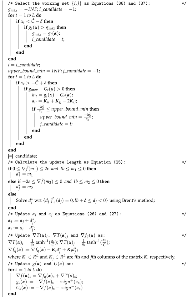until the stopping criterion (35) is satisfied as $m\left(\mathit{\alpha }\right)-M\left(\mathit{\alpha }\right)\le \tau$;$\phantom{(}$ Calculate $b:=\frac{1}{2}\left(\underset{s\in \left\{s|{\alpha }_s<\widehat{C}-\delta \right\}}{max}{g}_s\left(\mathit{\alpha }\right)+\underset{s\in \left\{s|{\alpha }_s>-\widehat{C}+\delta \right\}}{min}{G}_s\left(\mathit{\alpha }\right)\right)$

4. Experiments

This section considers the dual problem (14) of the proposed $\epsilon$-ln SVR, where a specific relationship holds between parameters ${\eta }_1$ and ${\eta }_2$ such as ${\eta }_2=\sqrt{\frac{1}{2}{\psi }_1\left(\frac{1}{2{\eta }_1}\right)}$. Tuning ${\eta }_1$ optimizes the loss function for a family of PHS distributions, as detailed in Section 2.2. To solve this challenging nonsmooth nonlinear dual problem (14) including linear equality and box constraints, a novel SMO-like algorithm with an efficient WSS procedure is introduced. This approach involves minimizing an upper bound on the second-order approximation, derived from the Taylor series expansion between consecutive loss function values.

For evaluating the $\epsilon$-ln SVR, comparisons are drawn against the $\epsilon$-$l_2$ SVR and the $\epsilon$-SVR, both respectively solved by SMO algorithms [21,52]. The proposed WSS procedure with SO-like information, which is one of the parts of the SMO-like algorithm that most affects the convergence time, is compared with its FO counterpart. Additionally, the proposed SMO algorithm for the nonsmooth dual problem is compared with the SMO algorithm for its smooth counterpart (7). All implementations are written in C++. The SMO-like algorithm presented in Algorithm 1 is adapted for use with the well-known LIBSVM library [52] to take advantage of its efficient kernel computation and caching mechanisms.

All experiments were carried out on a PC equipped with an Intel Core i5-12450H processor and 16 GB of RAM, operating on a 64-bit Windows 11 system. The RBF kernel, defined as $K({\mathit{x}}_s,{\mathit{x}}_r)=exp(-{\parallel {\mathit{x}}_s-{\mathit{x}}_r\parallel }^2/2{\sigma }^2)$, was used. A stopping criterion (35) with $\tau ={10}^{-3}$ and a cache size of 100 MB was set across all SMO algorithm implementations. Five-fold cross-validation was used to tune the regularization parameter, kernel parameter and ${\eta }_1$ within specified ranges $\left\{{10}^{-1},{10}^0,{10}^1,{10}^2,{10}^3\right\}$, $\left\{2^{-3},2^{-2},2^{-1},2^0,2^1\right\}$ and $\left\{2^{-3},2^{-2},\dots ,2^3\right\}$, respectively. The epsilon parameter was then chosen from a separate set $\left\{0,0.02,0.05,0.1,0.2,0.5,1,1.5,2,2.5,4\right\}$. The choice of the ${\eta }_1$ parameter range is based on the understanding of its influence on the lncosh loss function. As shown in Figure 1, smaller values of ${\eta }_1$ result in behavior similar to the $l_2$ loss, while larger values resemble the $l_1$ loss. This is consistent with the theoretical basis given in Equations (20) and (21), where the ${\eta }_1$ tuning covers the spectrum between Vapnik’s loss and the insensitive $l_2$ loss for its extreme values. In addition, Figure 1e shows the relationship between ${\eta }_1$ and the associated probability density function. In particular, ${\eta }_1=2^3$ and ${\eta }_1=2^{-3}$ lead to approximations of the Laplacian and Gaussian distributions, respectively. Based on these observations, we chose a range for ${\eta }_1$ that effectively captures this transition in the behavior of the loss function and the probability density. Root Mean Square Error (RMSE) was used for performance evaluation. Results are averages of four cross-validation repetitions, obtained by running three SVR variants on nine benchmark datasets. Among these datasets, Mpg, Housing, Space ga, Abalone and CpuSmall are accessible on the LIBSVM website (https://www.csie.ntu.edu.tw/~cjlin/libsvmtools/datasets/, accessed on 20 April 2024), while the remaining datasets were from the UCI machine-learning repository (https://archive.ics.uci.edu/datasets, accessed on 20 April 2024). While outputs remained unchanged, inputs were normalized to the closed interval $[0,1]$ due to varying dataset ranges. The outputs were also contaminated with additive Gaussian $N(0,0.04)$ and Cauchy noises $C(0,0.1)$ to compare the noise and outlier robustness of the proposed and traditional SVR variants. Iteration and training time ratios demonstrated in Figure 2 and Figure 3 are defined as follows:

$$\mathrm{iteration}\mathrm{ratio}=\frac{\#\mathrm{iter}.\mathrm{by}\mathrm{the}\mathrm{proposed}\mathrm{method}}{\#\mathrm{iter}\mathrm{by}\mathrm{other}\mathrm{method}}$$

$$\mathrm{training}\mathrm{time}\mathrm{ratio}=\frac{\mathrm{time}\mathrm{by}\mathrm{the}\mathrm{proposed}\mathrm{method}}{\mathrm{time}\mathrm{by}\mathrm{other}\mathrm{method}}$$

Table 1. A comparison of $\epsilon$-$l_2$ SVR, $\epsilon$-SVR and $\epsilon$-ln SVR.

Dataset	Method	(C, $\mathit{\sigma }$, $\mathit{\epsilon }$, ${\mathit{\eta }}_1$)	# of SVs	Test RMSE	Training Cpu Time	# of Iterations
Servo (167x4)	$\epsilon$-$l_2$ SVR	(${10}^1$, $2^0$, 0)	133.5 ± 0.53	0.886 ± 0.18	0.033 ± 0.04	459 ± 13.6
	$\epsilon$-SVR	(${10}^3$, $2^0$, $0.02$)	130.9 ± 1.79	0.785 ± 0.27	0.138 ± 0.03	57,100.2 ± 16,430.5
	$\epsilon$-ln SVR	(${10}^1$, $2^{-1}$, 0, $2^1$)	133.6 ± 0.52	0.726 ± 0.28	0.052 ± 0.04	1253 ± 53.5
Auto-mpg (392x7)	$\epsilon$-$l_2$ SVR	(${10}^1$, $2^{-1}$, $0.5$)	257.9 ± 7.23	2.776 ± 0.33	0.064 ± 0.03	1049.1 ± 37.7
	$\epsilon$-SVR	(${10}^2$, $2^{-1}$, $0.5$)	245.5 ± 4.06	2.674 ± 0.36	0.022 ± 0.03	5236.1 ± 938.0
	$\epsilon$-ln SVR	(${10}^1$, $2^{-1}$, $1.5$, $2^{-1}$)	160.2 ± 6.11	2.595 ± 0.27	0.039 ± 0.02	967.9 ± 88.9
Boston (560x13)	$\epsilon$-$l_2$ SVR	(${10}^2$, $2^0$, 0)	404.8 ± 0.42	4.626 ± 1.72	0.059 ± 0.03	4827.3 ± 106.9
	$\epsilon$-SVR	(${10}^2$, $2^0$, 1)	265.8 ± 8.32	3.461 ± 0.78	0.058 ± 0.05	4062.1 ± 820.9
	$\epsilon$-ln SVR	(${10}^2$, $2^{-1}$, 1, $2^1$)	269.3 ± 5.12	3.151 ± 0.38	0.061 ± 0.03	5261.9 ± 252.4
Cooling (768x8)	$\epsilon$-$l_2$ SVR	(${10}^1$, $2^0$, 0)	614.4 ± 0.52	3.031 ± 0.33	0.044 ± 0.03	2339.4 ± 59.1
	$\epsilon$-SVR	(${10}^2$, $2^{-1}$, 0)	614.4 ± 0.52	1.981 ± 0.20	0.222 ± 0.06	39,150.1 ± 4705.9
	$\epsilon$-ln SVR	(${10}^3$, $2^0$, 0, $2^{-3}$)	614.4 ± 0.52	1.772 ± 0.15	0.153 ± 0.08	65,277.4 ± 1747.3
Heating (768x8)	$\epsilon$-$l_2$ SVR	(${10}^2$, $2^0$, 0)	614.3 ± 0.67	1.980 ± 0.21	0.098 ± 0.02	9212.6 ± 213.4
	$\epsilon$-SVR	(${10}^3$, $2^0$, $0.5$)	421.9 ± 8.28	1.124 ± 0.10	0.621 ± 0.19	143,945.9 ± 27,282.0
	$\epsilon$-ln SVR	(${10}^3$, $2^0$, 0, $2^0$)	614.4 ± 0.52	0.939 ± 0.06	0.267 ± 0.07	91,786.0 ± 2373.9
Airfoil (1503x5)	$\epsilon$-$l_2$ SVR	(${10}^1$, $2^{-2}$, 0)	1202.4 ± 0.52	3.849 ± 1.32	0.083 ± 0.05	4840.6 ± 130.3
	$\epsilon$-SVR	(${10}^2$, $2^{-3}$, $0.2$)	1103.5 ± 5.97	2.776 ± 0.26	0.147 ± 0.08	28,317.0 ± 3876.7
	$\epsilon$-ln SVR	(${10}^2$, $2^{-2}$, 1, $2^{-1}$)	789.7 ± 9.52	2.778 ± 0.27	0.120 ± 0.03	15,367.1 ± 451.2
Space ga (3107x6)	$\epsilon$-$l_2$ SVR	(${10}^2$, $2^1$, 0)	2485.4 ± 0.70	1.232 ± 0.40	0.243 ± 0.03	8361.1 ± 655.1
	$\epsilon$-SVR	(${10}^1$, $2^{-2}$, $0.05$)	2184.9 ± 11.01	0.134 ± 0.01	0.508 ± 0.11	21,577.9 ± 2162.1
	$\epsilon$-ln SVR	(${10}^2$, $2^1$, 0, $2^0$)	2485.1 ± 0.74	0.116 ± 0.01	0.319 ± 0.06	20,649.9 ± 648.4
Abalone (4177x8)	$\epsilon$-$l_2$ SVR	(${10}^0$, $2^{-2}$, 0)	3341.2 ± 0.63	2.406 ± 0.22	0.308 ± 0.07	6336.3 ± 119.7
	$\epsilon$-SVR	(${10}^0$, $2^0$, $1.5$)	1367.8 ± 20.42	2.288 ± 0.12	0.156 ± 0.02	916.5 ± 29.2
	$\epsilon$-ln SVR	(${10}^1$, $2^1$, $1.5$, $2^2$)	1351.5 ± 19.13	2.208 ± 0.10	0.216 ± 0.06	8339.0 ± 594.8
Cpusmall (8192x12)	$\epsilon$-$l_2$ SVR	(${10}^1$, $2^0$, 0)	6553.3 ± 0.48	3.478 ± 0.17	3.411 ± 0.28	14,239.7 ± 127.7
	$\epsilon$-SVR	(${10}^1$, $2^{-1}$, 1)	4542.1 ± 28.83	3.257 ± 0.06	0.713 ± 0.28	5976.9 ± 445.6
	$\epsilon$-ln SVR	(${10}^1$, $2^{-1}$, $0.5$, $2^{-1}$)	5497.7 ± 16.87	3.126 ± 0.05	2.119 ± 0.53	48,499.2 ± 1151.9

shows a comparison of $\epsilon$-$l_2$ SVR, $\epsilon$-SVR and the proposed $\epsilon$-ln SVR variants. “# of SVs” is the number of support vectors identified by the model during training. “Test RMSE” represents the RMSE on the unseen test data, which evaluates the generalization performance of the model. “Training cpu time” indicates the computational time required to train the model on the training data. “# of iterations” indicates the number of iterations required for the SMO-like optimization algorithm described in Algorithm 1 to converge. “C” is the regularization parameter, which controls the trade-off between fitting the data and avoiding overfitting. “$\sigma$” is the kernel parameter, which controls the influence of the data points in the kernel function. “$\epsilon$” is the epsilon parameter, which defines the tolerance for errors within the $\epsilon$-insensitive zone of the SVR model. “${\eta }_1$” is a hyperparameter specific to the proposed $\epsilon$-ln SVR loss function, controlling the shape of the lncosh loss function as shown in Figure 1. The values of the hyperparameters (C, $\sigma$, $\epsilon$, ${\eta }_1$) differ between the SVR variants because the employed losses have different characteristics. The $l_2$ loss function lacks a bounded influence function and is weak in terms of outlier robustness. Therefore, it is observed that the value of the regularization parameter C for $\epsilon$-$l_2$ SVR is the lowest for most datasets to avoid overfitting, given that the datasets are contaminated with Cauchy and Gaussian noise. Additionally, it is noted that $\epsilon$-$l_2$ SVR tends to have the largest $\sigma$ for most datasets to mitigate the risk of overfitting, as a lower $\sigma$ results in a more localized influence, leading to complex fitting functions, especially in the presence of outliers and noise. To emphasize the influence of the tunable parameter ${\eta }_1$ within the lncosh loss function, datasets are selected from commonly used regression benchmarks, ensuring diversity in size and characteristics. The datasets are arranged in increasing order of training samples, ranging from small (e.g., Servo) to large (e.g., CpuSmall). Notably, datasets are chosen that exhibit a range of optimal ${\eta }_1$ values, as shown in Table 1. This selection allows us to demonstrate the effectiveness of the lncosh loss function and its tunability across diverse datasets.

While $\epsilon$-SVR and $\epsilon$-$l_2$ SVR employ loss functions optimized for specific noise distributions such as Laplace and Gaussian, respectively, the $\epsilon$-ln SVR offers greater flexibility. Its modified lncosh loss is optimal for the broader family of power-raised hyperbolic secant distributions, encompassing Laplace, Gaussian and hyperbolic secants as special cases. Moreover, as indicated in (20) and (21), the lncosh loss approaches Vapnik’s and $\epsilon$-insensitive $l_2$ losses for the limit values of ${\eta }_1$. For other values of ${\eta }_1$, it continues to exhibit its inherent properties, including robustness to noise and outliers. So, it effectively addresses outliers induced by Cauchy noise while also handling small noises mostly exhibiting Gaussian distribution. Therefore, the $\epsilon$-ln SVR has better test RMSE compared to $\epsilon$-SVR and $\epsilon$-$l_2$ SVR, as shown in Table 1, thanks to its ability to be optimal for different noise distributions by tuning ${\eta }_1$. While these results are an extension of the previous work [40], a computationally efficient SMO-like algorithm is provided to solve the nonsmooth nonlinear dual problem of $\epsilon$-ln SVR in order to handle larger datasets. Furthermore, it has been observed that solving such a complex nonsmooth nonlinear optimization problem (14) requires comparable training times as seen in Table 1 compared to solving the piecewise QP problems of $\epsilon$-$l_2$ SVR [21] and QP problems of $\epsilon$-SVR [52]. $\epsilon$-SVR and $\epsilon$-$l_2$ SVR have a well-defined analytical solution at each iteration for solving the subproblem consisting of two optimization parameters. Despite the lack of a direct analytical solution, the proposed SMO algorithm uses Brent’s method at each iteration to address this complex problem and provides acceptable training times through its easily computable WSS procedure. Due to its fast nature and single execution per iteration as demonstrated in Algorithm 1, Brent’s method contributes minimally to the overall running time of the algorithm.

The SMO algorithm solves the optimization problem iteratively by updating only two Lagrangian multipliers at each step. The choice of the right pair, known as the working set selection procedure, is crucial as it significantly affects the convergence speed. Therefore, the proposed WSS procedure with SO-like information, which is designed to minimize an upper bound on the second-order Taylor polynomial approximation of consecutive loss function values, is compared with the traditional WSS procedure with FO information. It is observed that the proposed SMO with easily computable WSS procedure significantly improves both the number of iterations and the training times compared to its FO counterpart, as shown in Figure 2. This is evident in all datasets, where both time and iteration ratios are consistently less than 1. The strength of the WSS procedure lies in its efficient retrieval of SO-like information. This allows it to prioritize pairs that maximize the decrease in consecutive loss function values. It achieves this by estimating an upper bound on the Taylor polynomial approximation, unlike the FO counterpart which simply uses gradient information. This often results in many more iterations for the FO counterpart because it lacks insight into the potential reduction in consecutive losses.

The proposed SMO algorithm is specifically designed to optimize dual convex nonsmooth problem (14) but it can also handle the smooth counterpart (7) as a special case. To demonstrate the effectiveness of the SMO algorithm for solving this nonsmooth formulation, we compare its performance to the smooth counterpart. As shown in Figure 3, SMO algorithm for solving this nonsmooth version consistently performs better, with iteration ratios close to 1 and training time ratios significantly less than 1 for all datasets. This stems from the smooth version’s SMO algorithm handling twice the number of optimization variables, requiring caching a larger kernel matrix of size $\mathit{K}\in R^{2L\times 2L}$ rather than $\mathit{K}\in R^{L\times L}$. The findings from comparing the proposed method with its FO and smooth counterparts are consistent with previous studies on SMO algorithms for solving piecewise QP problems in $\epsilon$-$l_2$ SVR [21] and $\epsilon$-SVR [22], but with the key distinction that the idea of minimizing an upper bound of the second-order Taylor polynomial approximation in WSS allows for a computationally efficient SMO algorithm even for this complex nonsmooth problem. Figure 2b and Figure 3b demonstrate the efficiency further, presenting ratios for total iterations and times during hyperparameter selection, again highlighting the method’s advantages across the different values of the hyperparameters.

The proposed SMO-like algorithm generalizes the classical SMO algorithm, designed for solving QP problems, to tackle more general nonsmooth, nonlinear convex dual problems arising in SVR with various loss functions. This generalization allows it to be adapted to both $\epsilon$-$l_2$ SVR and $\epsilon$-$l_1$ SVR. Due to the existence of analytical solutions for each iteration in the SMO-like algorithms for $\epsilon$-$l_2$ SVR and $\epsilon$-$l_1$ SVR, Brent’s method becomes unnecessary. Consequently, only the WSS part, a key innovation of our algorithm, is embedded into the SMO-like algorithms presented in [21,22]. As shown in Figure 4a,b, the iteration ratios for both $\epsilon$-$l_2$ SVR and $\epsilon$-$l_1$ SVR cases are exactly 1. This indicates that the proposed WSS, which leverages an upper bound based on the second-order Taylor polynomial approximation of consecutive loss function values, performs the same number of total iterations during hyperparameter selection for all datasets. Figure 4 presents the ratios for total times during hyperparameter selection. The proposed, easy-to-compute WSS described in Algorithm 1 demonstrates clear efficiency gains compared to those in [21,22], since time ratios are below 1 for all datasets. The efficiency comes from incorporating the concept of working set selection, which is associated with the second-order Taylor polynomial approximation, and defining an upper bound that is easy to compute, as described in Proposition 4. This enables the efficient use of SO-like information to effectively tackle SVR problems, even those involving complex nonsmooth nonlinear convex scenarios.

5. Discussion

In this study, we introduce the $\epsilon$-ln SVR model with a flexible lncosh loss function and demonstrate significant advances in its optimization and applicability. We derive a computationally efficient nonsmooth dual formulation of the problem, which addresses the challenges of nonlinearity and nondifferentiability. To overcome these complexities, a novel SMO-like algorithm with an effective WSS procedure is developed. This WSS procedure exploits second-order information by minimizing an upper bound on the Taylor polynomial approximation of consecutive loss function values, resulting in improved computational efficiency compared to its first-order and smooth counterparts. In addition, the single-parameter adjustable lncosh loss function is shown to be optimal in the maximum likelihood sense for the PHS distribution, which includes Laplace, Gaussian and hyperbolic secant distributions. This adjustable single-parameter design is shown to be advantageous for adaptation to unknown noise distributions in practical applications. Overall, the ability of the proposed SMO-like algorithm to handle a class of nonlinear convex problems demonstrates its potential applicability to SVR models with different loss functions optimized for different noise distributions and other related problems such as Lasso and Extreme Learning Machine. We expect that this innovative combination of $\epsilon$-ln SVR and an adapted SMO-like algorithm will pave the way for more robust and efficient SVR implementations with diverse loss functions that are optimal in the maximum likelihood sense for different noise distributions.

References

1. Smola, A.J.; Schölkopf, B. A tutorial on support vector regression. Stat. Comput. 2004, 14, 199–222. [Google Scholar] [CrossRef]
2. Vapnik, V.N. Statistical Learning Theory; John Wiley & Sons: New York, NY, USA, 1998. [Google Scholar]
3. Boser, B.; Guyon, I.; Vapnik, V.N. A training algorithm for optimal margin classifiers. In Proceedings of the Fifth Annual Workshop on Computational Learning Theory, Pittsburgh, PA, USA, 27–29 July 1992. [Google Scholar]
4. Cortes, C.; Vapnik, V.N. Support-vector network. Mach. Learn. 1995, 20, 273–297. [Google Scholar] [CrossRef]
5. Arnosti, N.A.; Kalita, J.K. Cutting Plane Training for Linear Support Vector Machines. IEEE Trans. Knowl. Data Eng. 2013, 25, 1186–1190. [Google Scholar] [CrossRef]
6. Chu, D.; Zhang, C.; Tao, Q. A Faster Cutting Plane Algorithm with Accelerated Line Search for Linear SVM. Pattern Recognit. 2017, 67, 127–138. [Google Scholar] [CrossRef]
7. Xu, Y.; Akrotirianakis, I.; Chakraborty, A. Proximal gradient method for huberized support vector machine. Pattern Anal. Appl. 2016, 19, 989–1005. [Google Scholar] [CrossRef]
8. Ito, N.; Takeda, A.; Toh, K.C. A unified formulation and fast accelerated proximal gradient method for classification. J. Mach. Learn. Res. 2017, 18, 1–49. [Google Scholar]
9. Majlesinasab, N.; Yousefian, F.; Pourhabib, A. Self-Tuned Mirror Descent Schemes for Smooth and Nonsmooth High-Dimensional Stochastic Optimization. IEEE Trans. Autom. Control 2019, 64, 4377–4384. [Google Scholar] [CrossRef]
10. Balasundaram, S.; Gupta, D.; Kapil. Lagrangian support vector regression via unconstrained convex minimization. Neural Netw. 2014, 51, 67–79. [Google Scholar] [CrossRef]
11. Balasundaram, S.; Yogendra, M. A new approach for training Lagrangian support vector regression. Knowl. Inf. Syst. 2016, 49, 1097–1129. [Google Scholar] [CrossRef]
12. Balasundaram, S.; Benipal, G. On a new approach for Lagrangian support vector regression. Neural Comput. Appl. 2018, 29, 533–551. [Google Scholar] [CrossRef]
13. Wang, H.; Shi, Y.; Niu, L.; Tian, Y. Nonparallel Support Vector Ordinal Regression. IEEE Trans. Cybern. 2017, 47, 3306–3317. [Google Scholar] [CrossRef]
14. Yin, J.; Li, Q. A semismooth Newton method for support vector classification and regression. Comput. Optim. Appl. 2019, 73, 477–508. [Google Scholar] [CrossRef]
15. Platt, J.C. Fast training of support vector machines using sequential minimal optimization. In Kernel Methods: Support Vector Machines; Schölkopf, B., Burges, C., Smola, A., Eds.; MIT Press: Cambridge, MA, USA, 1998. [Google Scholar]
16. Keerthi, S.S.; Shevade, S.K.; Bhattacharyya, C.; Murthy, K.R.K. Improvements to Platt’s SMO algorithm for SVM classifier design. Neural Comput. 2001, 13, 637–649. [Google Scholar] [CrossRef]
17. Fan, R.E.; Chen, P.H.; Lin, C.J. Working set selection using second order information for training support vector machines. J. Mach. Learn. Res. 2005, 6, 1889–1918. [Google Scholar]
18. Flake, G.W.; Lawrence, S. Efficient SVM regression training with SMO. Mach. Learn. 2002, 46, 271–290. [Google Scholar] [CrossRef]
19. Guo, J.; Takahashi, N.; Nishi, T. A novel sequential minimal optimization algorithm for support vector regression. In Neural Information Processing. ICONIP 2006. Lecture Notes in Computer Science; King, I., Wang, J., Chan, L.W., Wang, D., Eds.; Springer: Berlin/Heidelberg, Germany, 2006; pp. 827–836. [Google Scholar]
20. Takahashi, N.; Guo, J.; Nishi, T. Global convergence of SMO algorithm for support vector regression. IEEE Trans. Neural Netw. 2008, 19, 971–982. [Google Scholar] [CrossRef]
21. Kocaoğlu, A. An efficient SMO algorithm for Solving non-smooth problem arising in ε-insensitive support vector regression. Neural Process. Lett. 2019, 50, 933–955. [Google Scholar] [CrossRef]
22. Kocaoğlu, A. A sequential minimal optimization algorithm with second-order like information to solve a non-smooth support vector regression constrained dual problem. Uludağ Univ. J. Fac. Eng. 2021, 26, 1111–1120. [Google Scholar] [CrossRef]
23. Tang, L.; Tian, Y.; Yang, C.A. Nonparallel support vector regression model and its SMO-type solver. Neural Netw. 2018, 105, 431–446. [Google Scholar] [CrossRef]
24. Abe, S. Optimizing working sets for training support vector regressors by Newton’s method. In Proceedings of the International Joint Conference on Neural Networks, Killarney, Ireland, 12–17 July 2015. [Google Scholar]
25. Keerthi, S.S.; Shevade, S.K. SMO algorithm for least-squares SVM formulations. Neural Comput. 2003, 15, 487–507. [Google Scholar] [CrossRef]
26. Lopez, J.; Suykens, J.A.K. First and Second Order SMO Algorithms for LS-SVM Classifiers. Neural Process. Lett. 2011, 33, 31–44. [Google Scholar] [CrossRef]
27. Kumar, R.; Sinha, A.; Chakrabarti, S.; Vyas, O.P. A fast learning algorithm for one-class slab support vector machines. Knowl. Based Syst. 2021, 53, 107267. [Google Scholar] [CrossRef]
28. Gu, B.; Shan, Y.; Quan, X.; Zheng, G. Accelerating sequential minimal optimization via Stochastic subgradient descent. IEEE Trans. Cybern. 2021, 51, 2215–2223. [Google Scholar] [CrossRef] [PubMed]
29. Galvan, G.; Lapucci, M.; Lin, C.J. A two-Level decomposition framework exploiting first and second order information for SVM training problems. J. Mach. Learn. Res. 2021, 22, 1–38. [Google Scholar]
30. Huang, X.; Shi, L.; Suykens, J.A.K. Support vector machine classifier with pinball loss. IEEE Trans. Pattern Anal. Mach. Intell. 2014, 36, 984–997. [Google Scholar] [CrossRef] [PubMed]
31. Huang, X.; Shi, L.; Suykens, J.A.K. Sequential minimal optimization for SVM with pinball loss. Neurocomputing 2015, 149, 1596–1603. [Google Scholar] [CrossRef]
32. Huang, X.; Shi, L.; Suykens, J.A.K. Asymmetric least squares support vector machine classifiers. Comput. Stat. Data Anal. 2014, 70, 395–405. [Google Scholar] [CrossRef]
33. Farooq, F.; Steinwart, I. An SVM-like approach for expectile regression. Comput. Stat. Data Anal. 2017, 109, 159–181. [Google Scholar] [CrossRef]
34. Balasundaram, S.; Meena, Y. Robust Support Vector Regression in Primal with Asymmetric Huber Loss. Neural Process. Lett. 2019, 49, 1399–1431. [Google Scholar] [CrossRef]
35. Zhang, S.; Hu, Q.; Xie, Z.; Mi, J. Kernel ridge regression for general noise model with its application. Neurocomputing 2015, 149, 836–846. [Google Scholar] [CrossRef]
36. Prada, J.; Dorronsoro, J.R. General noise support vector regression with non-constant uncertainty intervals for solar radiation prediction. J. Mod. Power Syst. Clean Energy 2018, 6, 268–280. [Google Scholar] [CrossRef]
37. Wanga, Y.; Yang, L.; Yuan, C. A robust outlier control framework for classification designed with family of homotopy loss function. Neural Netw. 2019, 112, 41–53. [Google Scholar] [CrossRef] [PubMed]
38. Anand, P.; Khemchandani, R.R.; Chandra, S. A class of new support vector regression models. Appl. Soft Comput. 2020, 94, 106446. [Google Scholar] [CrossRef]
39. Dong, H.; Yang, L. Kernel-based regression via a novel robust loss function and iteratively reweighted least squares. Knowl. Inf. Syst. 2021, 63, 1149–1172. [Google Scholar] [CrossRef]
40. Karal, O. Maximum likelihood optimal and robust Support Vector Regression with lncosh loss function. Neural Netw. 2017, 94, 1–12. [Google Scholar] [CrossRef]
41. Kocaoğlu, A.; Karal, Ö.; Güzeliş, C. Analysis of chaotic dynamics of Chua’s circuit with lncosh nonlinearity. In Proceedings of the 8th International Conference on Electrical and Electronics Engineering, Bursa, Turkey, 28–30 November 2013. [Google Scholar]
42. Liu, C.; Jiang, M. Robust adaptive filter with lncosh cost. Signal Process. 2020, 168, 107348. [Google Scholar] [CrossRef]
43. Liang, T.; Li, Y.; Zakharov, Y.V.; Xue, W.; Qi, J. Constrained least lncosh adaptive filtering algorithm. Signal Process. 2021, 183, 108044. [Google Scholar] [CrossRef]
44. Liang, T.; Li, Y.; Xue, W.; Li, Y.; Jiang, T. Performance and analysis of recursive constrained least lncosh algorithm under impulsive noises. IEEE Trans. Circuits Syst. II 2021, 68, 2217–2221. [Google Scholar] [CrossRef]
45. Guo, K.; Guo, L.; Li, Y.; Zhang, L.; Dai, Z.; Yin, J. Efficient DOA estimation based on variable least Lncosh algorithm under impulsive noise interferences. Digital Signal Process. 2022, 122, 103383. [Google Scholar] [CrossRef]
46. Yang, Y.; Zhou, H.; Gao, Y.; Wu, J.; Wang, Y.-G.; Fu, L. Robust penalized extreme learning machine regression with applications in wind speed forecasting. Neural Comput. Appl. 2022, 34, 391–407. [Google Scholar] [CrossRef]
47. Zhao, H.; Wang, Z.; Xu, W. Augmented complex least lncosh algorithm for adaptive frequency estimation. IEEE Trans. Circuits Syst. II 2023, 70, 2685–2689. [Google Scholar] [CrossRef]
48. Yang, Y.; Zhou, H.; Wu, J.; Ding, Z.; Tian, Y.-C.; Yue, D.; Wang, Y.-G. Robust adaptive rescaled lncosh neural network regression toward time-series forecasting. IEEE Trans. Syst. Man Cybern. Syst. 2023, 53, 5658–5669. [Google Scholar] [CrossRef]
49. Faliva, M.; Zoia, M.G. A distribution family bridging the Gaussian and the Laplace laws, Gram–Charlier expansions, Kurtosis behaviour, and entropy features. Entropy 2017, 19, 149. [Google Scholar] [CrossRef]
50. Debruyne, M.; Hubert, H.; Suykens, J.A.K. Model selection in kernel based regression using the influence function. J. Mach. Learn. Res. 2008, 9, 2377–2400. [Google Scholar]
51. Bubeck, S. Convex Optimization: Algorithms and Complexity. Found. Trends Mach. Learn. 2015, 8, 231–357. [Google Scholar] [CrossRef]
52. Chang, C.C.; Lin, C.J. LIBSVM: A library for support vector machines software. ACM Trans. Intell. Syst. Technol. 2011, 2, 1–27. [Google Scholar] [CrossRef]
Figure 1. (a) The loss functions (9) for different values of η 1 with η 2 = 1 2 ψ 1 ( 1 2 η 1 ) and ε = 0 . (b) The loss functions with ε = 0.3 . (c,d) The first derivatives of the corresponding loss functions. (e,f) The associated probability density functions, which approximate Laplacian and Gaussian distributions for η 1 = 2 3 and η 2 = 2 3 , respectively. L ( 0 , 1 / 2 ) and N ( 0 , 1 ) denote Laplace and Gaussian distributions.
Applsci 14 03641 g001aApplsci 14 03641 g001b
Figure 2. Comparison of the proposed SMO algorithm with the novel WSS procedure, which provides SO-like information, and the SMO with the traditional WSS procedure, which provides FO information. Iteration and training time ratios are presented for (a) the optimal hyperparameters specified in Table 1 and (b) the hyperparameter selection procedure.
Applsci 14 03641 g002
Figure 3. Comparison of the proposed SMO algorithm for solving smooth (7) vs. nonsmooth (14) problems. Iteration and training time ratios are presented for (a) the optimal hyperparameters specified in Table 1 and (b) the hyperparameter selection procedure.
Applsci 14 03641 g003
Figure 4. Comparison of the proposed SMO-like algorithm: (a) Adapted to solve ε - l 2 SVR vs. the SMO-like algorithm introduced in [21] for hyperparameter selection procedure. (b) Adapted to solve ε - l 1 SVR vs. the SMO-like algorithm introduced in [22] for hyperparameter selection procedure.
Applsci 14 03641 g004