Abstract
Remotely sensed images provide effective sources for monitoring crop growth and the early prediction of crop productivity. To monitor carrot crop growth and yield estimation, three 27 ha center-pivot irrigated fields were studied to develop yield prediction models using crop biophysical parameters and vegetation indices (VIs) extracted from Sentinel-2A (S2) multi-temporal satellite data. A machine learning (ML)-based image classification technique, the random forest (RF) algorithm, was used for carrot crop monitoring and yield analysis. The VIs (NDVI, RDVI, GNDVI, SIPI, and GLI), extracted from S2 satellite data for the crop ages of 30, 45, 60, 75, 90, 105, and 120 days after plantation (DAP), and the chlorophyll content, SPAD (Soil Plant Analysis Development) meter readings, were incorporated as predictors for the RF algorithm. The RMSE of the five RF scenarios studied ranged from 7.8 t ha−1 (R2 ≥ 0.82 with Scenario 5) to 26.2 t ha−1 (R2 ≤ 0.46 with Scenario 1). The optimal window for monitoring the carrot crop for yield prediction with the use of S2 images could be achieved between the 60 DAP and 75 DAP with an RMSE of 8.6 t ha−1 (i.e., 12.4%) and 11.4 t ha−1 (16.2%), respectively. The developed RF algorithm can be utilized in carrot crop yield monitoring and decision-making processes for the self-sustainability of carrot production.
1. Introduction
The self-sustainability of a country’s food supply is essential for its economic growth and development. With the adoption of advanced techniques and available best management practices, Saudi Arabia is keen to expand the area of vegetable crops, especially carrots, to achieve self-sufficiency. Carrot (Daucus carota L.) is one of the most nutritionally valuable vegetable crops in the world, and carrot production has received great attention from researchers around the world, aiming to improve its production practices. The global production of carrots and turnips in 2021 was estimated at 42,158,403 tons out of a total cultivated area of 1,137,738 hectares, where Saudi Arabia produced 24,500 tons out of a total cultivated area of 1383 hectares [1]. Timely information on crop area and production statistics, agroclimatic regimes, real-time crop health monitoring, and yield prediction or pre-harvest modeling techniques will provide better options for food sustainability forecasts [2,3]. On the other hand, such data are crucial for improving agricultural practices and, subsequently, help decision-making authorities to effectively plan for food security issues and overcome unstable climatic conditions [4,5,6].
Investigating local variations in carrot yield and quality would enable decision-making, the implementation of agronomical guidance, and food self-sustainability. Nowadays, most of the decision support systems for agriculture practices are dependent on thematic maps, generated from moderate- to low-resolution satellite images [7,8]. Feature extraction and the assessment of the temporal dynamics of spectral information on agricultural lands are also crucial in decision processes [9,10,11]. Information and data analytics on seasonal crop conditions with periodic advisories on yield prediction in the early stages of the crop or before harvests are essential and allow a timely intervention to improve crop conditions [3,4]. Advanced remote-sensing techniques, multi-sensor satellite data, drones, mobile-based field data, and many other modeling techniques offer the opportunity to identify crop risk assessment, agro-advisory, yield assessment, and water use efficiency as well as solutions for farmer-centric and planning-centric activities in the agricultural decision-making process [2]. Spectral analyses such as vegetation indices, leaf area index (LAI), leaf chlorophyll content, etc., have been used to estimate the biophysical characteristics of plants [4,5,6]. For example, crop vegetation indices (VIs) extracted from satellite imagery, such as the normalized difference vegetation index (NDVI), soil-adjusted vegetation index (SAVI), and enhanced vegetation index (EVI), have been widely used for the early prediction of crop yields [12,13,14]. The VIs related to different crop growth parameters, such as plant cover (%), leaf area index (LAI), and chlorophyll and nitrogen contents, contribute to describing the growth status of different crops [15,16,17,18]. Numerous studies have proven the effectiveness of using various vegetation indices derived from multispectral wavebands to assess crop growth conditions and yield modeling in conjunction with ground-truth data on crop characteristics [3,10,11,12,13,14].
Schauberger et al. [19] reported the extent of studies on the yield forecasting of horticultural crops, while studies by Suarez et al. [20,21] described the importance of carrot yield forecasting and explored satellite images used for carrot yield prediction. Wei [22] generated carrot yield maps using planetScope hyperspectral data with a high accuracy (R2 = 0.68–0.82), and a study by de Lima Silva [23] achieved a good carrot predicted yield accuracy (R2 = 0.68) using planetScope CubeSat Platform. Similarly, studies [24,25] achieved carrot yields with a 33–35% variation using Landsat-8 and Sentinel-2 data, respectively. The successful prediction of crop yield depends mainly on the capability of sensors or images and the spectral response of a crop [26,27,28,29]. The crop yield variability can be assessed by addressing crop growth dynamics and multi-temporal data related to biophysical, physiological, or biochemical characteristics [30].
Fast and accurate information on crop phenology, crop health, crop water use, yield, etc. can be achieved with the use of deep-learning (DL) and artificial intelligence (AI) tools [31,32,33]. Machine learning (ML) is essential for improving the growth of the crop yield in a sustainable manner, helping to interpret and correlate field data with consumption techniques that can contribute to support decision-making in agriculture for crop health monitoring, agronomic suggestions, disease detection, weed-control, yield prediction, etc. [34,35,36]. Examples include sunflower [37], sugarcane [38], rice [39], corn [40], wheat [41], carrot [20,21,22], etc. The ML algorithms, including neural network (NN), stacked autoencoder (SAE), recurrent NN (RNN), graph NN (GNN), and restricted Boltzmann machine (RBM), have been widely used in agricultural applications [32]. Recently, machine-learning techniques, especially regression decision trees, random forest (RF) regression analysis, and artificial neural networks, have been widely used in the mapping and monitoring of crops [33,34,35,36]. One of the main advantages of machine learning is the development of a trained model that can be used to classify any scene so that the procedure can be partially or fully automated. Many authors applied deep-learning tools for the extraction of information from various satellite datasets, including Landsat-8, Sentinel-2, World View-2, hyperspectral, POLSAR (Polarimetric SAR), etc. [23,24,25,26,27,28,29].
Leaf chlorophyll content (LCC) is an important parameter to understanding the dynamic changes in physiological aspects and is highly related to crop health and productivity. To characterize the spatial variability of LCC in large fields, using traditional methods such as plant nutrient analysis is a laborious, cost-effective, and time-consuming process. Given the strong correlation between chlorophyll and nitrogen content in green vegetation, the non-destructive mode of chlorophyll measurements recorded with the Soil Plant Analysis Development—SPAD meter (SPAD-502, Minolta Osaka Company, Ltd., Osaka, Japan) is considered a reliable representation of LCC [42,43,44]. Recent studies used the SPAD reading in conjunction with remotely sensed images, such as Landsat, Sentinel-2, and drone images, for monitoring crop health conditions and spatial variation [44,45,46,47].
Satellites and ML algorithms have been used to predict crop production [20,21,22,23]. However, such studies are very limited, especially under dry climatic conditions. Hence, the current study, which aimed to monitor crop health and generate carrot pre-harvest yield models using machine-learning techniques, was formulated as part of the self-sustainability of vegetable crops and their water footprint. The main objective of this study was to address crop-monitoring strategies for crop phenology, health stress, and yield through the retrieval of leaf chlorophyll content (LCC) by combining the SPAD readings and remotely sensed Sentinel-2 multispectral data employing ML techniques. The specific objectives were (i) to retrieve the leaf chlorophyll content (LCC) of carrot fields by combining the SPAD readings and Sentinel-2 data for crop health monitoring and yield assessment, and (ii) to incorporate LCC data for the development of carrot yield forecasting algorithms using the random forest (RF) approach, a machine-learning (ML) tool.
2. Materials and Methods
2.1. Study Area and the Experimental Procedure
This study was conducted on three carrot fields irrigated with a center-pivot system (Fields’ IDs: N1, N4, and N6), each with an area of 27 hectares, belonging to the Tawdeehiya Farms located between the cities of Al-Kharj and Haradh in Saudi Arabia. This farm has an area of approximately 7000 ha and is located within an arid climatic zone between the latitudes of 24°10′22.77″ and 24°12′37.25″ N and the longitudes of 47°56′14.60″ and 48°05′08.56″ E (Figure 1). Sandy loam soil was the dominant soil type in the farm, where the main crops grown during the study period included a group of vegetables, the most important of which was the carrot crop. The mean annual temperatures in the experimental site ranged between 12 °C and 42 °C in the winter and summer seasons, respectively. The mean annual rainfall was about 98 mm, distributed mainly in the period between November and February. Tawdeehiya Farm produces carrots commercially and has facilities for data collection and measurements for continuous monitoring and yield assessment.
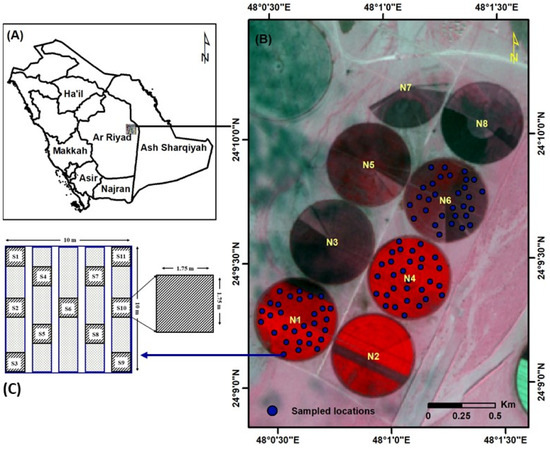
Figure 1.
Location map of Tawdeehiya Farms (A); experimental fields (B) and sampling strategy used for field data collection (C).
2.2. Carrot Cultivation
The experimental work was conducted for two carrot cultivation seasons. The first season was during the period from February to June 2021, while the second season was from October 2021 to January 2022 (Table 1). Before planting, soil beds (275 × 1.75 m) were prepared over the entire field, so each soil bed was managed with four plant rows. The carrot plant (variety: Soprano) was planted at a seeding rate of 4.0 kg ha−1 with a mean distance of 4.62 cm between two seeds in a row. A center-pivot irrigation system was used to provide irrigation water to the crop with an average water amount of 1197 and 1348 mm ha−1 for the first and second seasons, respectively.

Table 1.
Details of satellite images used for the study (DAP—Days after plantation; GDD—Growing degree days).
2.3. Sampling Strategy and Field Data Collection
A total of 90 permanent sampling locations in the three experimental fields (30 from each field) were randomly selected and georeferenced using a portable GPS receiver (Trimble Geo XH 6000, Trimble, Westminster, CO, USA). At each sampling location, a 10 m × 10 m plot was laid, which matches the pixel resolution of visible bands (i.e., blue, green, red, and NIR) of the S2 image (Figure 1). Soil samples (0–15 cm from the surface) and periodic field data were collected from the 90 sample plots (Figure 1C). For better data, soil samples were extracted from eleven sub-plots (1.75 m × 1.75 m) and were subsequently pooled as a composite sample. The soil samples were processed and analyzed for soil physicochemical properties (EC and pH). On the other hand, the carrot plant population was enumerated at 10–13 days after plantation (DAP).
2.3.1. SPAD Data and Leaf Samples for Tissue Analysis
Ground data collection of leaf chlorophyll over carrot fields was performed using a handheld SPAD meter, across the growth period (i.e., 30, 45, 60, 75, 90, 105, and 120 DAP). The measurements were recorded from five to ten mature leaves per sample from each of the 90 pre-determined sampling locations in the three experimental fields, as shown in Figure 1B, coinciding (±2 days) with the Sentinel-2 image acquisition dates/overpasses (Table 1). After the SPAD measurements, leaf samples were collected and subjected to laboratory analysis for total nitrogen (%).
2.3.2. Carrot Yield (YA)
Carrots were harvested at 125 DAP to 140 DAP from the pre-determined 90 sampling locations of the three experimental fields. After the harvest, crop parameters such as carrot length, diameter, and weight were measured. Approximately 6–9% of the carrots were found to be damaged or defective and omitted from the analysis. Carrots with a diameter of less than 3 mm, those that have deformed structures, or those that have visible physical damage were not considered when evaluating crop yield. Subsequently, the fresh weight of carrots was recorded and converted to yield (YA, tons/ha) for each experimental field.
2.3.3. Growing Degree Days (GDDs)
Growing degree days (GDDs) were computed to identify the phenological growth stages of carrot plants for the determination of the optimal window for effective growth and yield. Based on the accumulated GDD, season-wise collected data were categorized as seedling stage (SL), vegetative stage (VS), root development (RD), and root maturation (RM) stages. The GDDs were calculated using daily temperatures following Equation (1) provided by McMaster and Wilhelm [48]:
where Tmax and Tmin are the daily maximum and minimum temperatures, respectively. If the (Tmax + Tmin)/2 is less than the base, then GDD is equal to the base temperature (Tbase). The Tbase temperature was set to 4 °C in this study as described by McMaster and Wilhelm [48]. A cumulative GDD for each S2 image was computed by summing the calculated GDD values.
2.4. Satellite Data and Image Processing
Satellite images with 10 m resolution are preferably suitable for data analysis and modeling agricultural studies such as decision-making, practicing sustainable agriculture, and execution of site-specific management practices in fields [49]. Freely available data from Sentinel-2 fulfill the requirements, as it has both the 20 m and 10 m resolution spectral bands. Therefore, level 2A cloud-free Sentinel-2 (sensors A and B) satellite images were downloaded from the datahub of the European Space Agency (https://dataspace.copernicus.eu/; accessed on 9 February 2024). The downloaded S2 images were pre-processed and analyzed for surface reflectance using the SNAP software program (Ver. 3.4.1). Each band of processed images was resampled to 10 m pixel resolution. The individual bands (2, 3, 4, and 8A) and selected vegetation indices, VI (Table 2), were computed for the carrot crop monitoring and yield prediction employing the machine-learning (ML) algorithm such as random forest. As the study intended to predict carrot production, vegetation indices related to chlorophyll and vegetation analysis were incorporated for the modeling.
Table 2.
List of vegetation indices used for the study.
2.4.1. Retrieval of Leaf Chlorophyll Content (LCC)
As demonstrated in studies [42,43,44], SPAD readings were directly correlated with remotely sensed data, and feasible for the retrieval of LCC over carrot fields. A scatter plot was drawn between SPAD measurements and VIs derived from Sentinel-2 (S2) selected vegetation indices (VIs) and the performed regression analysis for the retrieval of LCC over carrot fields. We obtained imperial model for the simulation of LCC and expressed as Equation (2). The best-fit models were identified with coefficients of determination (R2) and root mean square error (RMSE), and, subsequently, based on the statistical analysis best or suitable vegetation index for upscaling of field-measured SPAD readings to simulated LCC layers. Thereafter, the simulated LCC layers were utilized in crop health assessment and the development of yield prediction models.
where a and b are the model parameters, i represents for number of models, and x indicates the studied vegetation index.
2.4.2. Preparation of Map for Carrot Crop Monitoring
A best-fit-model-generated simulated LCC layers were utilized for the preparation of maps for crop health monitoring by converting the LCC values to leaf nitrogen content. An empirical model was generated by performing the linear regression analysis between field-measured SPAD readings and the laboratory-analyzed leaf nitrogen content. Subsequently, the generated maps of carrot fields were used for fertilizer management and to identify the growth stage of carrots.
2.4.3. Random Forest (RF) Algorithm for Carrot Yield Prediction
A geodatabase of processed S2 images, time-series VIs, and LCC layers were developed. The recorded GPS co-ordinates generated a shape file of 90 sampling plots. Temporal changes in the spectral reflectance of carrot plants across the growing season were assessed and categorized as per the carrot growth stage. SNAP and ArcMap 10.8.1 were used to pre-process the data and build the models. Season-wise mean values of selected S2 bands, VIs, and LCC of each sampled location were extracted. Carrot crop monitoring and productivity zones of the three tested fields were assessed. As described in Boltan and Friedl [30], based on the phenology information (15, 30, 45, 60, 75, 90, 105, and 120 DAP), datasets were assessed. Due to cloud and haze coverage, and lack of availability of S2 images, the study ensured that at least one S2 image for each phenology stage. Subsequently, the interpolation was performed using the RF algorithm for spatial variation in crop development and yield was assessed at the field scale for productivity zones using a machine-learning-based regression tool of SNAP software (Figure 2). In recent years, various ML models have been developed to classify satellite images using large volumes of datasets. Random forest (RF), a popular ML approach, uses many subclasses to classify data subsets that are randomly picked from the input data [55].
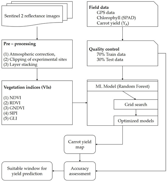
Figure 2.
Methodological flow of carrot crop monitoring and yield using machine-learning (ML) approach.
An RF algorithm is a supervised ML algorithm that is widely used for classification and regression problems in image analysis. The decision trees in the RF algorithm are the subclass classifiers. The RF procedure was performed in four steps, namely, (i) data preparation; (ii) model training with the use of Random Forest Classifier in SNAP software construction; training of carrot fields including variation in yield; (iii) averaging and voting of data by the decision tree; and (iv) selection of voting results and final prediction based on the bagging, meaning that the results so based on majority voting and model validation. The class with the most votes among the trees is introduced as the prediction output, and voting takes place among all of the trees’ predictions [56].
In this study, ML algorithms are driven to capture nonlinear relationships between the inputs (i.e., VIs, LCCs, etc.), and outputs (biophysical properties) through training datasets. The predictors used for the RF algorithm were ranked. These rankings were developed based on Pearson’s correlation coefficients, which were initially estimated to verify the association between carrot yield (YA) and Sentinel-2 bands (2, 3, 4, and 8A), vegetation indices (VIs), and SPAD values (i.e., LCCs). During the RF algorithm evaluation, five different categories of models were established based on the following: (a) S2 bands, (b) VIs, (c) a combination of S2 bands + VIs, (d) a combination of S2 bands + SPAD readings, and (e) a combination of S2 bands + VIs + SPAD values with correlation coefficient > 0.70).
2.5. Model Validation
During the prediction of results against the field-measured (SPAD and YA) data, the obtained dataset (90 samples) was randomly divided into two subsets of 63 samples (70% of the whole dataset) and 27 samples (30% of the whole dataset) for RF signature development and cross-validation, respectively. The 10-fold cross-validation resampling technique was used to tune the model hyper-parameters and to evaluate each model, considering the limited number of samples in the dataset [54]. The best-optimized models were tested against the remaining dataset (30%) that was not involved in the training-optimization phase. The range of the actual yield (YA) for each subset was inspected, based on the normal distribution curve, to ensure that the two subsets were not radically different. The strength of the developed models was determined through the coefficient of determination (R2) and the root mean square error (RMSE). The best-fit ML algorithms were utilized for the determination of the optimal crop growth stage useful for early forecasting of carrot yield.
3. Results
Descriptive statistics of the collected field data on soil EC, and soil pH, are presented in Table 3. The values of soil EC across the three experimental fields ranged from 1.23 to 3.27 dS m−1, with a coefficient of variation (CV) value of 41.4%, which indicates that the soil EC in the experimental field was relatively heterogeneous. The soil pH values, however, varied between 7.97 and 8.66 with a CV value of 1.91, indicating a homogeneous distribution of soil pH across the experimental fields. Based on the standard measures of soil EC and pH scales, the soil of the experimental field was characterized as non-saline and moderately alkaline. The ideal pH level for growing carrots is between 6.0 to 6.8 [57]. Hence, to the soils of the experimental fields were added wood ashes or dolomitic lime to balance the pH.
Table 3.
Soil electrical conductivity (EC, dSm−1) and pH of experimental fields.
The accumulated GDDs of the tested carrot crops varied between 333 at the seedling stage to 3374 at root maturation (i.e., 120 DAP). The GDD was higher (43%) in season 1 compared to season 2 (Figure 3). Phenological growth stages of carrot plants were assigned based on the GDD as the seedling stage-SS (GDD ≤ 948), vegetative growth stage-VS (GDD = 948 to 1215), root development stage-RD (1216 < GDD > 2210), and root maturation-RM (GDD > 2210) stages.
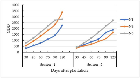
Figure 3.
Season-wise and field-wise growing degree days (GDD).
The carrot plant population, enumerated at 10–13 DAP, varied between 54.2 and 64.8 plants m−2, with a mean value of 58.5 and 61.1 plants m−2 for the first season (CV% = 18.4) and second season (CV% = 14.9), respectively (Table 4). The mean nitrogen content at harvest time was 2.09 g kg−1, where the minimum and maximum values were 1.31 g kg−1 and 2.58 g kg−1, respectively. The results indicated that the harvested carrot root yield (YA) ranged between 62.0 t ha−1 (Season-1) and 53.7 t ha−1 (Season-2), with a mean yield of 55.7 t ha−1 and a CV of 14%
Table 4.
Carrot parameters: root diameter, root length, fresh root weight, and carrot yield (YA).
The temporal advancement of LCC values measured by the SPAD meter is provided in Figure 4. The mean LCC values of carrot plant leaves increased sharply from 29.4 at a crop age of 30 days after planting (DAP) to 82.1 at 75 DAP, and then decreased to values of 73.3 at 90 DAP and dropped to 60.5 at 120 DAP (i.e., 15 ± 3 days before harvest), respectively. The seasonal dynamics of the studied VIs across the growing period of the carrot crop are provided in Figure 4. It was observed that approximately all the tested VIs (except the GLI) showed an increasing trend with carrot crop age, where they reached their peak values at a crop age of 60 DAP.
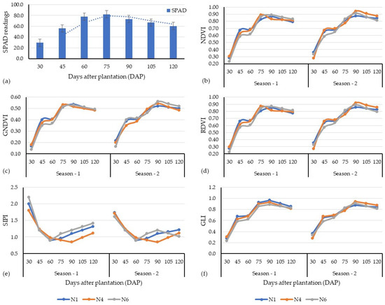
Figure 4.
Temporal variation in SPAD readings (a) and vegetation indices derived from Sentinel-2 image (b–f) across the growth stages (i.e., days after plantation).
3.1. Relationship between Leaf Nitrogen Concentration and SPAD Readings
A regression analysis between SPAD values and leaf nitrogen content showed a consistent relationship (R2 = 0.68; p < 0.001) as given in Figure 5. The leaf nitrogen content and the relationship with the SPAD readings are in accordance with the study by [58]. However, there is a variation in the significance of the model with other studies. It is due to the continuous observation of the SPAD, and laboratory analysis of nitrogen compared to others. On the other hand, SPAD values and the greenness of the leaf are significantly correlated, alternately depending on the rate of fertilizer application.
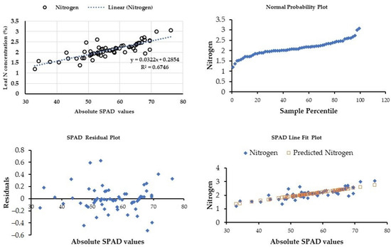
Figure 5.
Leaf nitrogen concentration (%) vs. absolute SPAD values across the carrot growth stages.
3.2. Relationship between SPAD Readings and Vegetation Indices (VIs)
Single VI-based best-fit models were assessed and provided in Table 5. The relationship between the simulated ground-measured SPAD readings and studied VIs was found to be significant with GNDVI (R2 = 0.78; p < 0.001), while a weak relationship was noticed with GLI (R2 = 0.09; p < 0.05). The best-fit models are observed with the peak stage of carrot growth at 60 DAP to 70 DAP. The correlation was low with all the studied VI earlier than 45 DAP, while, during the later stage (i.e., 90 DAP onwards), the results expressed a moderate correlation with RDVI and SIPI (Table 5).
Table 5.
Summary of coefficients of determination analysis between ground-measured SPAD readings and vegetation indices from Sentinel-2 data.
3.3. Random Forest Models for Carrot Monitoring and Yield Management
To identify the most suitable VI for the prediction of carrot yield (YP, t/ha), the actual carrot yield (YA) and the corresponding VIs were subjected to linear regression modeling, performed using XLStat (Ver. 19), a statistics software program, compatible with MS Excel. Linear regression results showed three models with a significant correlation between the VIs and the YA, with R2 values ranging between 0.51 and 0.66 (Figure 6). Out of the studied VIs, the RDVI, the SIPI, and the GNDVI were identified as the most suitable VIs for the growth assessment and yield of carrot crops. Subsequently, RDVI and GNDVI along with field-measured SPAD values were used as inputs in the execution of machine-learning algorithms, such as random forest (RF), for the determination of the crop growth and productivity (yield) management zones of the studied carrot fields. A summary of the dynamics of the carrot crop was monitored using S2 data, and yield prediction maps were generated based on the five scenarios (Figure 7).
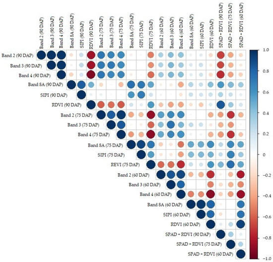
Figure 6.
A correlation plot that shows the dependence between the applied predictors based on the Pearson correlation coefficient. Dark blue colors indicate positive correlation, dark red colors indicate negative correlation, and near-white colors indicate weak or null correlation.
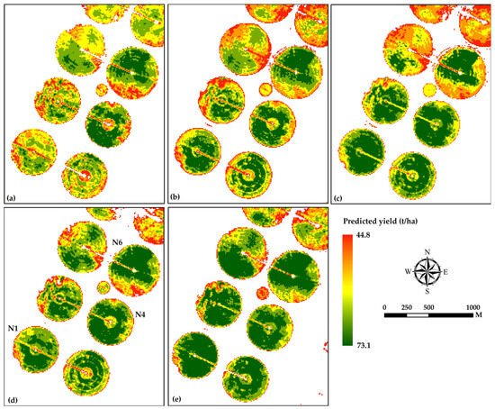
Figure 7.
Predicted carrot yield maps generated using a random forest (RF) algorithm. (a) Sentinel-2 bands, (b) vegetation indices, (c) Sentinel-2 bands + SPAD values, (d) vegetation indices + SPAD values, and (e) Sentinel-2 bands + vegetation indices + SPAD values, as predictors in model development. The SPAD values used in the model were with the Pearson correlation coefficient (R2) > 70 with yield (YA).
4. Discussion
4.1. Carrot Crop Growth Assessment
The results are in agreement with the literature, with regard to the capability of the selected S2 bands alone (Band 2, Band 3, Band 4, and Band 8A) to extract useful information about the carrot plant (health, and growth monitoring) status and crop yield prediction (R2 ≥ 0.62, %RMSE ≤ 24) [21]. Moreover, the use of the SIPI index with S2 bands improved the performance of ML prediction models. Using the average value of each band or index reported in [21], the ML algorithms can be used to predict the carrot yields at 70 DAS with an error of 27%. They also reported that the GNDVI and RDVI are the best VIs for the early prediction of yield. Band 8A was found to have a better predictive ability in the early prediction of yield with the R2 of 0.68, and it conformed with the study by Wei et al. [22]. RDVI relies on the reflectance information provided in the red and NIR region of the spectrum, retrieving in one of the absorption peaks of chlorophyll and b. Nevertheless, Wei et al. [22] identified other photosynthetic pigments in carrot plants whose absorption peaks are located in the blue region of the spectrum. The carrot crop was monitored throughout the growth period with the help of chlorophyll content (i.e., SPAD readings) across the DAS. In general, higher SPAD readings indicate a higher relative chlorophyll content and higher tissue nitrogen content, while lower SPAD readings indicate a lower relative chlorophyll content and lower tissue nitrogen content. As per Figure 4a, the SPAD readings reached their peak at 60 DAP and followed a similar trend at 75 DAP. Thereafter, the SPAD values dropped. The progressive increment in SPAD readings is due to the healthy condition of the crop and agricultural practices that are implemented. Furthermore, factors such as moisture, salt stress, etc. alter the vital function of the plants, resulting in a decrease in the SPAD readings [50]. Nitrogen maps were created using the simulated LCC of 75 DAP, as most of the studied VIs were found to be significant with SPAD readings, still suitable for the farmer to obtain location-specific information of crop N status in order to apply a side dressing. The crop development at 90 DAP does not express large variation effects with VIs alone, whereas the model combined with simulated LCC expressed significant correlation. Therefore, it is recommended that we co-combine the SPAD meter readings with progressing with the development of the crop, due to the effect of the crop development and increased vigor, which is an indicator of plant health and nutrient status. SPAD meter readings can be used to monitor the nutrient status of the corn crop and adjust fertilizer application rates accordingly.
4.2. ML Algorithm in Yield Assessment
The S2 bands 2, 3, 4, and 8A were used for the Scenario a RF algorithm; Band 2 and Band 8A performed well compared to Bands 4 and 8A. As depicted in Figure 7, however, the performance of the RF model executed using the vegetation indices, NDVI, alone as a parameter was not significant, whereas other VIs performed well at 45, 60, and 75 DAP. The combination of SPAD and RDVI (Model e) had a different impact on both the 60 and 75 DAP in RF algorithms. In most of the models, Band 3 was found to be more predictive for the crop age 60–90 DAP, and the GNDVI and SIPI for the crop age 75 and 90 DAP, respectively. The RDVI performed well for the crop age 60–75 DAP and was found to be more predictable for carrot yield (Figure 8). The generated RF models were appropriate in the yearly prediction of carrot yield with an optimal window of 60 to 75 DAP. Moreover, with the inclusion of biophysical parameter SPAD values, similar spatial patterns are observed in both the d and f models, coinciding in terms of spatial variability in the experimental fields. The GLI index covers both blue and red bands to derive the overall photosynthetic activity of the plant regardless of the pigment; the green band may also be a good proxy to measure the chlorophyll a concentration [59], and the SIPI index to assess water stress in carrots [60] can be achieved at R2 of 0.79 along with SPAD values [61,62].
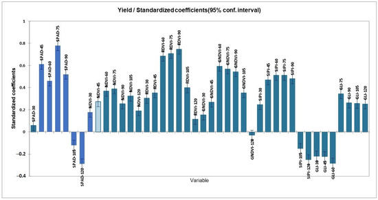
Figure 8.
Standards coefficients for the generation of carrot yield maps generated using a random forest (RF) algorithm.
The model performance statistics are discussed as shown in Table 6. Of the studied five scenarios (Models a–e), an algorithm with the maximum predictors (i.e., Scenario e), including individual S2 bands + VIs + SPAD values, performed well (R2 = 0.82; RMSE = 7.8 t ha−1) compared to other scenarios (a–d). The second-best model with an input of VIs and SPAD values (Scenario d) has resulted in a moderate correlation (R2 = 0.67; RMSE = 10.2 t ha−1). A poor performance (R2 = 0.46; RMSE = 26.2 t ha−1) was noted with Scenario a, i.e., only individual S2 bands as inputs for the RF model. It may be due to the impact of the feature selection process to reduce collinearity among predictors; it was also noticed that the RF model (d) was slightly improved compared to the other RF models (a–c) after the removal of non-correlated variables.
Table 6.
Summary of the best models (ML algorithm, variable predictors, and feature selection) and the corresponding values of accuracy indicators (R2 and RMSE).
Furthermore, Model e confirmed that the incorporation of LCC in ML modeling improves the model performance and reduces the bias from 26.2 t ha−1 to 7.8 t ha−1 (Table 6). It is attributed with the correlation between the temporal profile of the in situ measured chlorophyll (SPAD values), and the harvested carrot yield was reported to be moderate at 60 DAP (R2 = 0.46; p > 0.0001) and 90 DAP (R2 = 0.52; p > 0.0001). As depicted in Figure 9, a crop age of 75 DAP (R2 = 0.78; p < 0.0001) was found to be suitable for the early prediction of carrot yield using the SPAD values. The correlation between the temporal profile of vegetation indices and the harvested carrot yield (YA) varied across the VIs. As depicted in Figure 9, carrot yield was positively correlated and showed a moderate (R2 = 0.59; p < 0.001) to high significance (R2 = 0.74; p < 0.001) for GNDVI and RDVI, at the DAP of 60 to 90, respectively. On the other hand, SIPI also performed satisfactorily (R2 = 0.51; p > 0.001), while the correlation was moderately low with NDVI and GLI. When the simulated LCC layers were incorporated to the ML model, the performance of the model was superior compared to the models those did not include LCC layers for the early prediction of carrot yield. The summer prediction is given in Table 7.
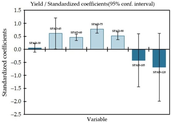
Figure 9.
Standards of coefficients between carrot yield and simulated LCC layers for yield prediction in RF algorithm.
Table 7.
Summary of coefficients of determination analysis between SPAD and harvested carrot yield (YA, t ha−1).
Nevertheless, to characterize the spatial variability of nitrogen in large fields, using traditional methods such as plant nutrient analysis and the simulated LCC developed based on ground-measured SPAD readings may enhance the performance of crop-monitoring and yield prediction models at convenient DAPs matching with the overpass of remotely sensed images. Hence, this study confirmed the strong correlation between the chlorophyll and nitrogen content in green vegetation; remote-sensing techniques in conjunction with SPAD readings have the potential to assess the spatial variability in large agricultural fields at lower costs than destructive traditional methods. On the other hand, SPAD readings and remotely sensed images such as Sentinel-2 have been used together to map chlorophyll content. Nevertheless, the center of the red band in Sentinel-2 is close to the absorption peaks of chlorophyll a and b at 662 nm and 644 nm; the SPAD measurements were captured at the red (650 nm) and infrared (940 nm) bands [60]. Therefore, Model e performed well with the incorporation of SPAD readings compared to other models and is in accordance with the recent study [63], which explained the use of SPAD values in improving the yield estimation model for walnuts combining the spectral indices, texture indices, and structural indices. Another study by Han et al. [64] on winter wheat revealed the ability of VIs to identify different aspects of plants and improved prediction performance (R2 = 0.807) by combining multispectral remote-sensing data with LAI and SPAD values. Hence, the best model (e) can be applied to monitor carrot fields and their seasonal dynamics and predict carrot yield in the study region and similar climates, which enhances the opportunities for sustainable management.
5. Conclusions
In this study, an attempt was made to identify the optimum window for the early prediction of carrot yield. The specific conclusions of the study include the following:
- The correlation between chlorophyll (SPAD values) content and carrot yield (YA) was found to be significant (R2 = 0.78; p = 0.0001) at a crop age of 75 DAP. However, a weak correlation was reported at 30 DAP (R2 = 0.058; p = 0.493) and 105 DAP (R2 = 0.42; p = 0.416).
- To monitor the development of carrot crops and to assess the optimal window for the early prediction of carrot yield, five scenarios/models adopting the RF algorithm, a machine-learning tool, were performed. Of the studied five scenarios, the algorithm with the maximum predictors (individual S2 bands + VIs + SPAD values) performed better (R2 = 0.82; RMSE = 7.8 t ha−1) compared to other scenarios, whereas the model with an input of VIs and SPAD values returned a moderate correlation (R2 ≤ 0.67; RMSE = 10.2 t ha−1). A poor performance (R2 ≥ 0.46; RMSE = 26.2 t ha−1) was noted with Scenario 1, i.e., only individual S2 bands as inputs for the RF model.
- Furthermore, Model e confirmed that the incorporation of LCC in ML modelling improves the model performance and reduces the bias from 10.4 t ha−1 to 52 t ha−1. Hence, the current study aimed to monitor the growth and assess and model the carrot pre-harvest yield using machine-learning techniques. The optimal period for the early management of carrot crops was found to be between 60–75 DAP and was formulated as part of the self-sustainability of vegetable crops and their water footprint. This study assists in exploring the possibilities of non-destructive methods, such as SPAD measurements and free-of-cost Sentinel-2 data in monitoring the growth and assessment of carrot yield employing ML techniques.
Author Contributions
Conceptualization, R.M. and K.A.A.-G.; methodology, R.M., K.A.A.-G., and E.T.; software, R.M., and M.K.E.; validation, E.T., and K.A.A.-G.; formal analysis, R.M. and H.F.E.; investigation, E.T.; resources, R.M.; data curation, M.K.E., H.F.E., A.A.A., and R.M.; writing—original draft preparation, R.M.; writing—review and editing, R.M., K.A.A.-G., and E.T.; visualization, K.A.A.-G.; supervision, R.M.; project administration, K.A.A.-G.; funding acquisition, R.M. All authors have read and agreed to the published version of the manuscript.
Funding
This research was funded by the National Plan for Science, Technology and Innovation (MAARIFAH/GRANTS program), King Abdul Aziz City for Science and Technology, Riyadh, Saudi Arabia, through the project number 2-17-04-001-0016, and the Article processing charges (APC) was also funded by the project number 2-17-04-001-0016.
Institutional Review Board Statement
Not applicable.
Informed Consent Statement
Not applicable.
Data Availability Statement
The Sentinel images used in this study are openly available at https://dataspace.copernicus.eu/browser/ (accessed on 9 February 2024). Other data used to support the findings of this study are available from the corresponding author upon request.
Acknowledgments
The authors are grateful to the National Plan for Science Technology and Innovation (MAARIFAH/GRANTS program), King Abdul Aziz City for Science and Technology, Riyadh, Saudi Arabia for funding this study. The unstinted co-operation and support extended by the Farm manager and the supporting staff in carrying out the field research work at the Tawdeehiya Farms are gratefully acknowledged.
Conflicts of Interest
The authors declare no conflicts of interest.
References
- FAOSTAT. Food and Agriculture Organization Corporate Statistical Database. 2021. Available online: http://www.fao.org/faostat/en/#data/QC (accessed on 20 November 2023).
- Gomez, D.; Salvador, P.; Sanz-Justo, J.; Casanova, J.-L. Potato yield prediction using machine learning techniques and sentinel 2 data. Remote Sens. 2019, 11, 1745. [Google Scholar] [CrossRef]
- Ennouri, K.; Kallel, A. Remote sensing: An advanced technique for crop condition assessment. Math. Prob. Eng. 2019, 2019, 9404565. [Google Scholar] [CrossRef]
- Tucker, C.J. Red and photographic infrared linear combinations for monitoring vegetation. Remote Sens. Environ. 1979, 8, 127–150. [Google Scholar] [CrossRef]
- Moran, M.S.; Inoue, Y.; Barnes, E.M. Opportunities and limitations for image-based remote sensing in precision crop management. Remote Sens. Environ. 1997, 61, 319–346. [Google Scholar] [CrossRef]
- Lobell, D.B. The use of satellite data for crop yield gap analysis. Field Crops Res. 2013, 143, 56–64. [Google Scholar] [CrossRef]
- Benami, E.; Jin, Z.; Carter, M.R.; Ghosh, A.; Hijmans, R.J.; Hobbs, A.; Kenduiywo, B.; Lobell, D.B. Uniting remote sensing, crop modeling and economics for agricultural risk management. Nat. Rev. Earth Environ. 2021, 2, 140–159. [Google Scholar] [CrossRef]
- Skakun, S.; Vermote, E.; Franch, B.; Roger, J.C.; Kussul, N.; Ju, J.; Masek, J. Winter wheat yield assessment from landsat 8 and sentinel-2 data: Incorporating surface reflectance, through phenological fitting, into regression yield models. Remote Sens. 2019, 11, 1768. [Google Scholar] [CrossRef]
- Battude, M.; AlBitar, A.; Morin, D.; Cros, J.; Huc, M.; Sicre, C.M.; LeDantec, V.; Demarez, V. Estimating maize biomass and yield over large areas using high spatial and temporal resolution Sentinel-2 like remote sensing data. Remote Sens. Environ. 2016, 184, 668–681. [Google Scholar] [CrossRef]
- Perich, G.; Turkoglu, M.O.; Graf, L.V.; Wegner, J.D.; Aasen, H.; Walter, A.; Liebisch, F. Pixel-based yield mapping and prediction from sentinel-2 using spectral indices and neural networks. Field Crops Res. 2023, 292, 108824. [Google Scholar] [CrossRef]
- Kamath, P.; Patil, P.; Shrilatha, S.; Sushma; Sowmya, S. Crop yield forecasting using data mining. Glob. Transit. Proc. 2021, 2, 402–407. [Google Scholar] [CrossRef]
- Atzberger, C. Advances in remote sensing of agriculture: Context description, existing operational monitoring systems and major information needs. Remote Sens. 2013, 5, 949–981. [Google Scholar] [CrossRef]
- Sheffield, K.; Morse-McNabb, E. Using satellite imagery to assess trends in soil and crop productivity across landscapes. IOP Conf. Ser. Earth Environ. Sci. 2015, 25, 012013. [Google Scholar] [CrossRef]
- Miller, G.J.; Dronova, I.; Oikawa, P.Y.; Knox, S.H.; Windham-Myers, L.; Shahan, J.; Stuart-Haentjens, E. The Potential of Satellite Remote Sensing Time Series to Uncover Wetland Phenology under Unique Challenges of Tidal Setting. Remote Sens. 2021, 13, 3589. [Google Scholar] [CrossRef]
- Dhillon, M.S.; Dahms, T.; Kuebert-Flock, C.; Rummler, T.; Arnault, J.; Steffan-Dewenter, I.; Ullmann, T. Integrating random forest and crop modeling improves the crop yield prediction of winter wheat and oil seed rape. Front. Remote Sens. 2023, 3, 1010978. [Google Scholar] [CrossRef]
- Myneni, R.; Williams, D. On the relationship between FAPAR and NDVI. Remote Sens. Environ. 1994, 49, 200–211. [Google Scholar] [CrossRef]
- Bala, S.K.; Islam, A.S. Correlation between potato yield and MODIS-derived vegetation indices. Int. J. Remote Sens. 2009, 30, 2491–2507. [Google Scholar] [CrossRef]
- Al-Gaadi, K.A.; Hassaballa, A.A.; Tola, E.; Kayad, A.G.; Madugundu, R.; Alblewi, B.; Assiri, F. Prediction of potato crop yield using precision agriculture techniques. PLoS ONE 2016, 11, e0162219. [Google Scholar] [CrossRef] [PubMed]
- Schauberger, B.; Jagermeyr, J.; Gornott, C. A systematic review of local to regional yield forecasting approaches and frequently used data resources. Eur. J. Agron. 2020, 120, 126153. [Google Scholar] [CrossRef]
- Suarez, L.A.; Robson, A.; McPhee, J.; O’Halloran, J.; van Sprang, C. Accuracy of carrot yield forecasting using proximal hyperspectral and satellite multispectral data. Precis. Agric. 2020, 21, 1304–1326. [Google Scholar] [CrossRef]
- Suarez, L.A.; Robertson-Dean, M.; Brinkhoff, J.; Robson, A. Forecasting carrot yield with optimal timing of Sentinel 2 image acquisition. Precis. Agric. 2023, 25, 570–588. [Google Scholar] [CrossRef]
- Wei, M.C.F.; Maldaner, L.F.; Ottoni, P.M.N.; Molin, J.P. Carrot Yield Mapping: A Precision Agriculture Approach Based on Machine Learning. AI 2020, 1, 229–241. [Google Scholar] [CrossRef]
- de Lima Silva, Y.K.; Furlani, C.E.A.; Canata, T.F. AI-Based Prediction of Carrot Yield and Quality on Tropical Agriculture. AgriEngineering 2024, 6, 361–374. [Google Scholar] [CrossRef]
- Al-Gaadi, K.A.; Madugundu, R.; Tola, E.; El-Hendawy, S.; Marey, S. Satellite-Based Determination of the Water Footprint of Carrots and Onions Grown in the Arid Climate of Saudi Arabia. Remote Sens. 2022, 14, 5962. [Google Scholar] [CrossRef]
- Madugundu, R.; Al-Gaadi, K.A.; Tola, E.; Hassaballa, A.A.; Kayad, A.G. Utilization of Landsat-8 data for the estimation of carrot and maize crop water footprint under the arid climate of Saudi Arabia. PLoS ONE 2018, 13, e0192830. [Google Scholar] [CrossRef] [PubMed]
- Roznik, M.; Boyd, M.; Porth, L. Improving crop yield estimation by applying higher resolution satellite NDVI imagery and high-resolution cropland masks. Remote Sens. Appl. Soc. Environ. 2022, 25, 100695. [Google Scholar] [CrossRef]
- Panda, S.S.; Ames, D.P.; Panigrahi, S. Application of Vegetation Indices for Agricultural Crop Yield Prediction Using Neural Network Techniques. Remote Sens. 2010, 2, 673–696. [Google Scholar] [CrossRef]
- Baez-Gonzalez, A.D.; Kiniry, J.R.; Maas, S.J.; Tiscareno, M.L.; Macias, J.C.; Mendoza, J.L.; Richardson, C.W.; Salinas, J.G.; Manjarrez, J.R. Large-area maize yield forecasting using leaf area index based yield model. Agron. J. 2005, 97, 418–425. [Google Scholar] [CrossRef]
- Lobell, D.B.; Ortiz-Monasterio, J.I.; Asner, G.P.; Naylor, R.L.; Falcon, W.P. Combining field surveys, remote sensing, and regression trees to understand yield variations in an irrigated wheat landscape. Agron. J. 2005, 97, 241–249. [Google Scholar] [CrossRef]
- Bolton, D.K.; Friedl, M.A. Forecasting crop yield using remotely sensed vegetation indices and crop phenology. Agric. Forest Meteorol. 2013, 173, 74–84. [Google Scholar] [CrossRef]
- Jhajharia, K.; Mathur, P. Prediction of crop yield using satellite vegetation indices combined with machine learning approaches. Adv. Space Res. 2023, 9, 3998–4007. [Google Scholar] [CrossRef]
- Crane-Droesch, A. Machine learning methods for crop yield prediction and climate change impact assessment in agriculture. Environ. Res. Lett. 2018, 13, 114003. [Google Scholar] [CrossRef]
- Geetha, V.; Punitha, A.; Abarna, M.; Akshaya, M.; Illakiya, S.; Janani, A.P. An Effective Crop Prediction Using Random Forest Algorithm. In Proceedings of the 2020 International Conference on System, Computation, Automation and Networking (ICSCAN), Pondicherry, India, 3–4 July 2020; pp. 1–5. [Google Scholar] [CrossRef]
- Gilbertson, J.K.; Van Niekerk, A. Value of dimensionality reduction for crop differentiation with multi-temporal imagery and machine learning. Compu. Electron. Agric. 2017, 142, 50–58. [Google Scholar] [CrossRef]
- Akbari, E.; Darvishi Boloorani, A.; Neysani Samany, N.; Hamzeh, S.; Soufizadeh, S.; Pignatti, S. Crop Mapping Using Random Forest and Particle Swarm Optimization based on Multi-Temporal Sentinel-2. Remote Sens. 2020, 12, 1449. [Google Scholar] [CrossRef]
- Wei, P.; Ye, H.; Qiao, S.; Liu, R.; Nie, C.; Zhang, B.; Song, L.; Huang, S. Early Crop Mapping Based on Sentinel-2 Time-Series Data and the Random Forest Algorithm. Remote Sens. 2023, 15, 3212. [Google Scholar] [CrossRef]
- Fieuzal, R.; Bustillo, V.; Collado, D.; Dedieu, G. Estimation of Sunflower Yields at a Decametric Spatial Scale—A Statistical Approach Based on Multi-Temporal Satellite Images. Proceedings 2019, 18, 7. [Google Scholar] [CrossRef]
- Everingham, Y.; Sexton, J.; Skocaj, D.; Inman-Bamber, G. Accurate prediction of sugarcane yield using a random forest algorithm. Agron. Sustain. Dev. 2016, 36, 27. [Google Scholar] [CrossRef]
- Narasimhamurthy, V.; Kumar, P. Rice Crop Yield Forecasting Using Random Forest Algorithm. Int. J. Res. Appl. Sci. Eng. Technol. 2017, 5, 1220–1225. [Google Scholar] [CrossRef]
- Ngie, A.; Ahmed, F. Estimation of Maize grain yield using multispectral satellite data sets (SPOT 5) and the random forest algorithm. S. Afr. J. Geomat. 2018, 7, 11–30. [Google Scholar] [CrossRef]
- Pantazi, X.E.; Moshou, D.; Alexandridis, T.; Whetton, R.L.; Mouzaen, A.M. Wheat yield prediction using machine learning and advanced sensing techniques. Comput. Electron. Agric. 2016, 121, 57–65. [Google Scholar] [CrossRef]
- Demmig-Adams, B.; Adams, W.W., III; Barker, D.H. Chlorophyll fluorescence as a tool in photosynthesis research. Photosyn. Res. 1996, 47, 1–10. [Google Scholar]
- Gitelson, A.A.; Merzlyak, M.N. Signature analysis of leaf reflectance spectra: Algorithm development for remote sensing of chlorophyll. J. Plant Physiol. 1994, 154, 448–456. [Google Scholar] [CrossRef]
- Priyanka, D.; Srivastava, P.K.; Rawat, R. Retrieval of leaf chlorophyll content using drone imagery and fusion with Sentinel-2 data. Smart Agric. Technol. 2023, 6, 100353. [Google Scholar] [CrossRef]
- Zhou, X.; Zhang, J.; Chen, D.; Huang, Y.; Kong, W.; Yuan, L.; Ye, H.; Huang, W. Assessment of Leaf Chlorophyll Content Models for Winter Wheat Using Landsat-8 Multispectral Remote Sensing Data. Remote Sens. 2020, 12, 2574. [Google Scholar] [CrossRef]
- Clevers, J.G.P.W.; Kooistra, L.; Van den Brande, M.M.M. Using Sentinel-2 Data for Retrieving LAI and Leaf and Canopy Chlorophyll Content of a Potato Crop. Remote Sens. 2017, 9, 405. [Google Scholar] [CrossRef]
- Guermazi, E.; Wali, A.; Ksibi, M. Combining remote sensing, SPAD readings, and laboratory analysis for monitoring olive groves and olive oil quality. Precis. Agric. 2024, 25, 65–82. [Google Scholar] [CrossRef]
- McMaster, G.S.; Wilhelm, W. Growing degree-days: One equation, two interpretations. Agric. Forest Meteorol. 1997, 87, 291–300. [Google Scholar] [CrossRef]
- Mulla, D.J. Twenty Five Years of Remote Sensing in Precision Agriculture: Key Advances and Remaining Knowledge Gaps. Biosyst. Eng. 2013, 114, 358–371. [Google Scholar] [CrossRef]
- Rouse, J.W.; Haas, R.H.; Schell, J.A.; Deering, D.W. Monitoring Vegetation Systems in the Great Plains with ERTS. In 3rd Earth Resource Technology Satellite (ERTS); NASA: Washington, DC, USA, 1974; Volume 1, pp. 48–62. [Google Scholar]
- Rougean, J.-L.; Breon, F.M. Estimating PAR absorbed by vegetation from bidirectional reflectance measurements. Remote Sens. Environ. 1995, 51, 75–384. [Google Scholar] [CrossRef]
- Gitelson, A.A.; Kaufman, Y.J.; Merzlyak, M.N. Use of a green channel in remote sensing of global vegetation from EOS-MODIS. Remote Sens. Environ. 1996, 58, 89–298. [Google Scholar] [CrossRef]
- Penuelas, J.; Baret, F.; Filella, I. Semi-Empirical Indices to Assess Carotenoids/Chlorophyll a Ratio from Leaf Spectral Reflectance. Photosynthetica 1995, 31, 221–230. [Google Scholar]
- Eng, L.S.; Ismail, R.; Hashim, W.; Baharum, A. The use of VARI, GLI, and VIgreen formulas in detecting vegetation in aerial images. Int. J. Tech. 2019, 10, 13851394. [Google Scholar] [CrossRef]
- Ghorbanian, A.; Kakooei, M.; Amani, M.; Mahdavi, S.; Mohammadzadeh, A.; Hasanlou, M. Improved land cover map of Iran using Sentinel imagery within Google Earth Engine and a novel automatic workflow for land cover classification using migrated training samples. ISPRS J. Photogram. Remote Sens. 2020, 167, 276–288. [Google Scholar] [CrossRef]
- Brownlee, J. Better Deep Learning: Train Faster, Reduce Overfitting, and Make Better Predictions; Machine Learning Mastery: Victoria, Australia, 2018. [Google Scholar]
- Scornet, E.; Biau, G.; Vert, J.-P. Consistency of random forests. Ann. Statist. 2015, 43, 1716–1741. [Google Scholar] [CrossRef]
- Radhamani, R.; Kannan, R. Nondestructive and rapid estimation of leaf chlorophyll content of sugarcane using a SPAD meter. Int. J. Sci. Res. 2016, 5, 2392–2397. [Google Scholar]
- Szeląg-Sikora, A.; Sikora, J.; Niemiec, M.; Gródek-Szostak, Z.; Kapusta-Duch, J.; Kuboń, M.; Komorowska, M.; Karcz, J. Impact of Integrated and Conventional Plant Production on Selected Soil Parameters in Carrot Production. Sustainability 2019, 11, 5612. [Google Scholar] [CrossRef]
- Markwell, J.; Osterman, J.C.; Mitchell, J.L. Calibration of the Minolta SPAD-502 leaf chlorophyll meter. Photosynth. Res. 1995, 46, 467–472. [Google Scholar] [CrossRef] [PubMed]
- Liu, C.; Liu, Y.; Lu, Y.; Liao, Y.; Nie, J.; Yuan, X.; Chen, F. Use of a leaf chlorophyll content index to improve the prediction of above-ground biomass and productivity. Peer J. 2019, 6, e6240. [Google Scholar] [CrossRef] [PubMed] [PubMed Central]
- Kandel, B.P. Spad value varies with age and leaf of maize plant and its relationship with grain yield. BMC Res. Notes 2020, 13, 475. [Google Scholar] [CrossRef] [PubMed]
- Wang, R.; Tuerxun, N.; Zheng, J. Improved estimation of SPAD values in walnut leaves by combining spectral, texture, and structural information from UAV-based multispectral image. Sci. Hortic. 2024, 328, 112940. [Google Scholar] [CrossRef]
- Han, X.; Wei, Z.; Chen, H.; Zhang, B.; Li, Y.; Du, T. Inversion of Winter Wheat Growth Parameters and Yield Under Different Water Treatments Based on UAV Multispectral Remote Sensing. Front. Plant Sci. 2021, 12, 609876. [Google Scholar] [CrossRef] [PubMed]
Disclaimer/Publisher’s Note: The statements, opinions and data contained in all publications are solely those of the individual author(s) and contributor(s) and not of MDPI and/or the editor(s). MDPI and/or the editor(s) disclaim responsibility for any injury to people or property resulting from any ideas, methods, instructions or products referred to in the content. |
© 2024 by the authors. Licensee MDPI, Basel, Switzerland. This article is an open access article distributed under the terms and conditions of the Creative Commons Attribution (CC BY) license (https://creativecommons.org/licenses/by/4.0/).