Fast and Highly Accurate Zonal Wavefront Reconstruction from Multi-Directional Slope and Curvature Information Using Subregion Cancelation

Abstract

The wavefront reconstruction is a crucial step in determining the performance of wavefront detection instruments. The wavefront reconstruction algorithm is primarily evaluated in three dimensions: accuracy, speed, and noise immunity. In this paper, we propose a hybrid zonal reconstruction algorithm that introduces slope and curvature information in the diagonal, anti-diagonal, horizontal, and vertical directions by dividing the neighbor sampling points into subregions in groups of four. By canceling the same parameters in integration equations, an algorithm using multi-directional slope–curvature information is achieved with only two sets of integration equations in each subregion, reducing the processing time. Simulation experiments show that the relative root-mean-square reconstruction error of this algorithm is improved by about 4 orders of magnitude compared with existing algorithms that use multi-directional slope information or slope–curvature information alone. Compared with the hybrid multi-directional slope–curvature algorithm, the proposed algorithm can reduce computation time by about 50% as well as provide better noise immunity and reconstruction accuracy. Finally, the validity of the proposed algorithm is verified by the null test experiment.

1. Introduction

The Shack–Hartmann wavefront sensor is one of the most widely used wavefront sensors because of its great energy utilization, fast real-time sensing, and strong anti-noise ability [1]. It is widely employed in the detection of human eye aberrations [2,3], astronomical observation [4,5], laser beam purification [6,7], optical element identification [8,9], and other fields. To enhance detection performance, researchers have modified the instrument structure to introduce more information and proposed slope and curvature hybrid sensors, which have significant research value. The selection of the reconstruction algorithm is of great importance to the performance of wavefront sensors in various application areas. To meet the practical engineering requirements, the reconstruction time should be shortened as much as possible while satisfying the reconstruction accuracy requirements and ensuring good noise resistance to adapt to various measurement environments [10,11,12,13,14,15,16,17].

Researchers have modified the classic zonal reconstruction method to improve the performance of the reconstruction method even further. On the one hand, a breakthrough point may be the discovery of a novel difference operator creation approach using mathematical methods. For example, Li et al. [18] employed the one-dimensional Taylor’s law to integrate the relationship among wavefront value, slope, and curvature, with smaller truncation errors. However, the arrangement of sample points affects reconstruction accuracy and noise immunity. Viegers et al. [19] enhanced the approximation accuracy of the difference operator in the interpolation process by inserting a spline function. Nonetheless, this approach is solved using an iterative method that requires a long computing time and shows relatively poor noise immunity. On the other hand, increasing the amount of measurement information in the reconstruction algorithm can improve reconstruction accuracy and noise immunity. For example, Barwick et al. [20] proposed the least-squares reconstruction method, which utilizes slope, Laplacian curvature, and torsional curvature information comprehensively. This method effectively improves the noise resistance, and the calculation speed is relatively fast, but the reconstruction accuracy could be improved further. To obtain additional data for reconstruction, Pathak et al. [21] incorporated the diagonal phase and slope into the zonal reconstruction. Based on the work of Li et al. [18], Zhong et al. [22] modified the method using the difference operator by introducing more information into the reconstruction process, which could not only increase the accuracy of the reconstruction algorithm but also improved its noise immunity. However, the algorithm increased the reconstruction time due to the addition of a new set of integral equations, and the error of the diagonal integration equation increased due to the increase in sampling point interval, both of which have the potential for further improvement.

As a result, to better meet the three criteria of the reconstruction algorithm indicated above, this paper proposes a fast slope–curvature hybrid reconstruction algorithm. By dividing the surroundings of the reconstruction point into multiple subregions, an integration equation with the minimum truncation error can be constructed for each subregion. This can be achieved using the Taylor expansion method. The integration equations of adjacent subregions are pairwise canceled to introduce first-order and second-order derivative information in the horizontal, vertical, diagonal, and anti-diagonal directions. Through the cancelation, more wavefront reconstruction information can be introduced while ensuring that the computational complexity remains unchanged, thereby improving the accuracy of wavefront estimation. By following the above steps, the fast slope–curvature hybrid reconstruction algorithm based on the subregion method proposed in this paper not only reduces the reconstruction time but also enhances the accuracy and noise resistance of wavefront estimation. This means that higher-order aberrations can be measured more accurately, enabling more precise optical measurement or image reconstruction.

The remaining parts of this paper are arranged as follows. Section 2 provides a detailed introduction to the Southwell operator, the geometric model, and the fast slope–curvature hybrid reconstruction algorithm based on the subregion method process. It also includes mathematical derivations of the formulas involved in the algorithm. Furthermore, error analysis is conducted to theoretically demonstrate the advantages of the proposed algorithm by introducing multiple pieces of information through subregion cancelation. In Section 3, the specific performance of the algorithm is simulated and compared with the currently prevailing hybrid reconstruction algorithms. The results are then discussed. In Section 4, the null test experiment of the four-hole amplitude-modulated wavefront sensor is completed, and the effectiveness of the proposed algorithm is verified. Finally, Section 5 provides a summary of the whole paper.

2. Principle of the Proposed Algorithm and Analysis of Its Residual Errors

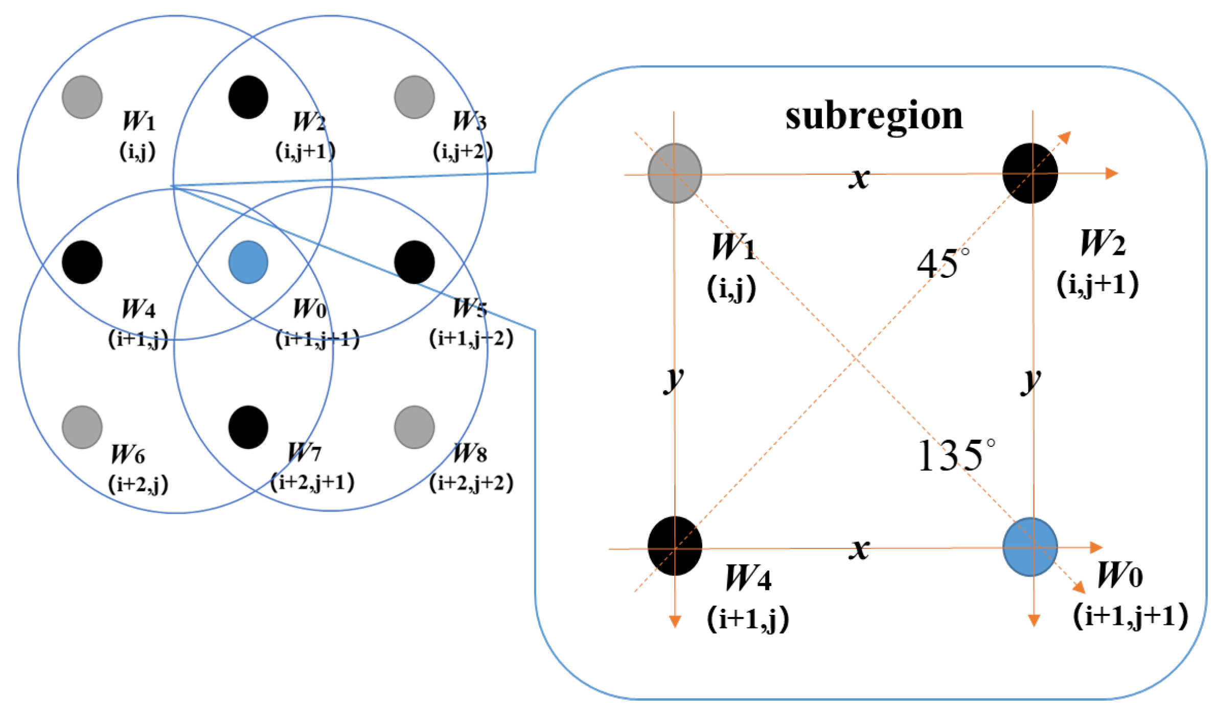
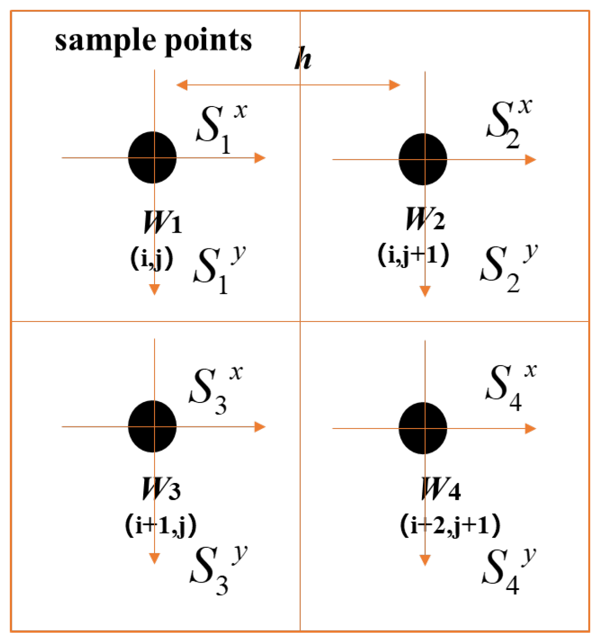
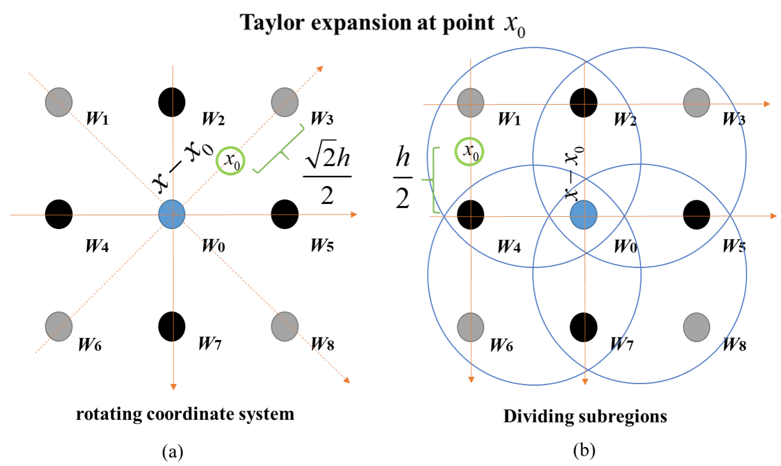
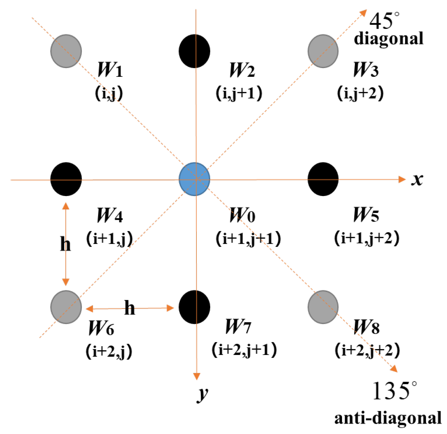
2.1. Principle and Process of the Proposed Algorithm

The zonal method represents the recovered wavefront through a linear combination of gradient information near each sampling point, and the least-squares solution is obtained by solving a linear system of equations. Take the most widely used Southwell model as an example, shown in Figure 1.

Using Newtonian interpolation integrals at two adjacent points, two sets of integration equations in the horizontal and vertical directions are obtained as follows:

$$\begin{array}{c}{W}_2-W_1=h\frac{\left(S_1^x+S_2^x\right)}{2},\\ \\ W_3-W_1=h\frac{\left(S_1^y+S_3^y\right)}{2},\end{array}$$

(1)

where W_n represents the wavefront value at position n of the sampling point, h is the sampling interval, and S_n^x and S_n^y represent the slope values of the wavefront in the x and y directions.

To further introduce more reconstruction information and thus improve the reconstruction package accuracy, Zhong et al. [22] used Taylor expansion to introduce second-order curvature information based on the Southwell model, which only utilizes first-order gradient information in the horizontal and vertical directions, to improve the reconstruction accuracy. Meanwhile, sampling points in the diagonal and anti-diagonal directions are also introduced to improve the reconstruction noise immunity.

As shown in Figure 2, the XY coordinate system is rotated by 45° to obtain the integration equations in the diagonal and anti-diagonal directions using a typical nine-sample point as an example as follows:

$$\begin{array}{c}{W}_5-W_0=h\times \frac{({S_5}^x+{S_0}^x)}{2}+h^2\times \frac{({C_5}^{xx}+{C_0}^{xx})}{12},\hfill \\ W_7-W_0=h\times \frac{({S_7}^y+{S_0}^y)}{2}+h^2\times \frac{({C_7}^{yy}+{C_0}^{yy})}{12},\hfill \\ W_3-W_0=\sqrt{2}h\times \frac{({S_3}^{+}+{S_0}^{+})}{2}+2h^2\times \frac{({C_3}^{+}+{C_0}^{+})}{12},\hfill \\ W_8-W_0=\sqrt{2}h\times \frac{({S_8}^{-}+{S_0}^{-})}{2}+2h^2\times \frac{({C_3}^{-}+{C_0}^{-})}{12},\hfill \end{array}$$

(2)

where

$$\begin{array}{c}{S_n}^{+}=\frac{\left(S_n^x+{S_n}^y\right)}{\sqrt{2}},\hfill \\ {S_n}^{-}=\frac{\left(S_n^x-{S_n}^y\right)}{\sqrt{2}},\hfill \\ {C_n}^{+}=\frac{C_n^{xx}}{2}+C_n^{xy}+\frac{C_n^{yy}}{2},\hfill \\ {C_n}^{-}=\frac{C_n^{xx}}{2}-C_n^{xy}+\frac{C_n^{yy}}{2},\hfill \end{array}$$

(3)

$\mathit{C}{\mathit{n}}^{xx}$ represents the curvature in the x direction, $\mathit{C}{\mathit{n}}^{yy}$ represents the curvature in the y direction, and $\mathit{C}{\mathit{n}}^{xy}$ represents the twist curvature term at position n of the sampling point. The first two equations in Equation (2) represent the reconfiguration relationships in the horizontal and vertical directions, and the second two equations represent the reconfiguration relationships in the diagonal and anti-diagonal directions.

By comparing Equations (1) and (2), we can see that the algorithm increases the number of integration equations compared to the traditional Southwell method, thus increasing the number of operations and computation time. The integration equations in the diagonal and anti-diagonal directions improve the noise immunity but increase the sampling interval, which affects the reconstruction accuracy.

To solve the above problems, based on the above two models, this paper proposes a new way of constructing the difference operator. By dividing the sampling area into subregions in groups of four points, the first- and second-order derivative information in the diagonal and antagonistic directions is introduced in the integration equations by canceling the same parameters, thus shortening the sampling interval in the reconstruction process in the diagonal and antagonistic directions, as shown in Figure 3.

Figure 2. Geometric schematic of the hybrid wavefront reconstruction algorithm using multi-directional slope and curvature information.

Figure 2. Geometric schematic of the hybrid wavefront reconstruction algorithm using multi-directional slope and curvature information.

Figure 3. Geometric schematic of proposed algorithm.

Figure 3. Geometric schematic of proposed algorithm.

Firstly, a Taylor expansion is used in the horizontal and vertical directions in the divided subregions to obtain a relationship between the wavefront with minimum truncation error and the first- and second-order derivatives of the sampling points, as derived below.

$$A{W}_1+B{W}_2=h\times (E{S}_1+F{S}_2)+h^2\times (G{C}_1+H{C}_2),$$

(4)

where ${\mathit{W}}_{\mathit{n}}$ represents the estimated wavefront at the sample location, ${\mathit{S}}_{\mathit{n}}$ represents the first-order derivative at location n along the adjacent sampling direction, ${\mathit{C}}_{\mathit{n}}$ represents the second-order derivative at location n along the adjacent sampling direction, expands both sides of Equation (4) at the same time at the sample midpoint Taylor location, and lets the coefficients of the same terms corresponding to both sides of the equation be equal to solve for the following:

$$W_2-W_1=\frac{h}{2}\times (S_1+S_2)+\frac{h^2}{12}\times (C_1-C_2),$$

(5)

Secondly, to introduce information on sampled points in the diagonal and anti-diagonal directions, four sets of reconstruction relations are obtained in turn using Equation (5) within the subregions consisting of the four points divided as described in Figure 3.

$$\begin{array}{c}{W}_{i,j+1}-W_{i,j}=\frac{h}{2}\left(S_{i,j+1}^x+S_{i,j}^x\right)+\frac{h^2}{24}\left(C_{i,j}^{xx}-C_{i,j+1}^{xx}\right),\hfill \\ W_{i+1,j+1}-W_{i+1,j}=\frac{h}{2}\left(S_{i+1,j+1}^x+S_{i+1,j}^x\right)+\frac{h^2}{12}\left(C_{i+1,j}^{xx}-C_{i+1,j+1}^{xx}\right),\hfill \\ W_{i+1,j}-W_{i,j}=\frac{h}{2}\left(S_{i+1,j}^y+S_{i,j}^y\right)+\frac{h^2}{12}\left(C_{i,j}^{yy}-C_{i+1,j}^{yy}\right),\hfill \\ W_{i+1,j+1}-W_{i,j+1}=\frac{h}{2}\left(S_{i+1,j+1}^y+S_{i,j+1}^y\right)+\frac{h^2}{12}\left(C_{i,j+1}^{yy}-C_{i+1,j+1}^{yy}\right),\hfill \end{array}$$

(6)

where i represents the row position of the sampled point, and j represents the column position of the sampled point. Add the four equations in Equation (6) and divide by two to obtain the first equation in Equation (7). Add the first and third equations in Equation (6) and subtract the second and fourth equations and divide by 2 to obtain the second equation in Equation (7).

$$\begin{array}{c}{W}_{i+1,j+1}-W_{i,j}=\frac{h}{4}\left(\begin{array}{c}{S}_{i,j+1}^x+S_{i,j}^x\hfill \\ +S_{i+1,j+1}^x+S_{i+1,j}^x\hfill \\ +S_{i+1,j}^y+S_{i,j}^y\hfill \\ +S_{i+1,j+1}^y+S_{i,j+1}^y\hfill \end{array}\right)+\frac{h^2}{24}\left(\begin{array}{c}{C}_{i,j}^x-C_{i,j+1}^x\hfill \\ +C_{i+1,j}^x-C_{i+1,j+1}^{xx}\hfill \\ +C_{i,j+1}^y-C_{i+1,j+1}^y\hfill \\ +C_{i,j}^y-C_{i+1,j}^y\hfill \end{array}\right),\\ W_{i,j+1}-W_{i+1,j}=\frac{h}{4}\left(\begin{array}{c}{S}_{i,j+1}^x+S_{i,j}^x\hfill \\ +S_{i+1,j+1}^x+S_{i+1,j}^x\hfill \\ -S_{i+1,j}^y-S_{i,j}^y\hfill \\ -S_{i+1,j+1}^y-S_{i,j+1}^y\hfill \end{array}\right)+\frac{h^2}{24}\left(\begin{array}{c}{C}_{i,j}^x-C_{i,j+1}^x\hfill \\ +C_{i+1,j}^x-C_{i+1,j+1}^x\hfill \\ -C_{i,j+1}^y+C_{i+1,j+1}^y\hfill \\ -C_{i,j}^y+C_{i+1,j}^y\hfill \end{array}\right),\end{array}$$

(7)

Equation (7) is the newly constructed difference operator in each subregion. By comparing with Equation (2), it can be seen that the algorithm proposed in this paper introduces sampling information in four directions using only two sets of equations, reducing the computational effort while ensuring the introduction of the same amount of information.

After obtaining the newly reconstructed difference operator, Equation (7) is extended to all sampling points and, written in the form of a matrix, yields

$$UW=V,$$

(8)

where U is the coefficient matrix, W is the wavefront matrix, and V is the slope and curvature matrix in the form of

$$\begin{array}{c}\hfill U={\left[\begin{array}{ccccc}{A}_1& A_2& & & \\ & A_1& A_2& & \\ & & \dots & \dots & \\ & & & A_1& A_2\\ B_1& B_2& & & \\ & B_1& B_2& & \\ & & \cdots & \cdots & \\ & & & B_1& B_2\end{array}\right]}_{2(N-1)\times N}\\ \hfill A_2=-B_1=\left[\begin{array}{cc}O\hfill & I_{N-1}\hfill \end{array}\right],\\ \hfill B_2=-A_1=\left[\begin{array}{cc}{I}_{N-1}\hfill & O\hfill \end{array}\right],\end{array}$$

$$W={\left[\begin{array}{ccccccccccc}{W}_{1,1}\hfill & W_{2,1}\hfill & \dots \hfill & W_{N,1}\hfill & W_{1,2}\hfill & \dots \hfill & W_{N,2}\hfill & \dots \hfill & W_{1,N}\hfill & \dots \hfill & W_{N,N}\hfill \end{array}\right]}^T$$

$$V=\left[\begin{array}{c}\frac{h}{4}\left(\begin{array}{c}{S}_{1,1}^x+S_{1,2}^x\hfill \\ +S_{2,1}^x+S_{2,2}^x\hfill \\ +S_{1,1}^y+S_{1,2}^y\hfill \\ +S_{2,1}^y+S_{2,2}^y\hfill \end{array}\right)+\frac{h^2}{24}\left(\begin{array}{c}{C}_{1,1}^{xx}-C_{1,2}^{xx}\hfill \\ +C_{2,1}^{xx}-C_{2,2}^{xx}\hfill \\ +C_{1,2}^{yy}-C_{2,2}^{yy}\hfill \\ +C_{1,1}^{yy}-C_{2,1}^{yy}\hfill \end{array}\right)\\ \dots \\ \frac{h}{4}\left(\begin{array}{c}{S}_{N,1}^x+S_{N,2}^x\hfill \\ +S_{N+1,1}^x+S_{N+1,2}^x\hfill \\ +S_{N,1}^y+S_{N,2}^y\hfill \\ +S_{N+1,1}^y+S_{N+1,2}^y\hfill \end{array}\right)+\frac{h^2}{24}\left(\begin{array}{c}{C}_{N,1}^{xx}-C_{N,2}^{xx}\hfill \\ +C_{N+1,1}^{xx}-C_{N+1,2}^{xx}\hfill \\ +C_{N,2}^{yy}-C_{N+1,2}^{yy}\hfill \\ +C_{N,1}^{yy}-C_{N+1,1}^{yy}\hfill \end{array}\right)\\ \dots \\ \frac{h}{4}\left(\begin{array}{c}{S}_{1,N}^x+S_{1,N+1}^x\hfill \\ +S_{2,N}^x+S_{2,N+1}^x\hfill \\ +S_{1,N}^y+S_{1,N+1}^y\hfill \\ +S_{2,N}^y+S_{2,N+1}^y\hfill \end{array}\right)+\frac{h^2}{24}\left(\begin{array}{c}{C}_{1,N}^{xx}-C_{1,N+1}^{xx}\hfill \\ +C_{2,N}^{xx}-C_{2,N+1}^{xx}\hfill \\ +C_{1,N+1}^{yy}-C_{2,N+1}^{yy}\hfill \\ +C_{1,N}^{yy}-C_{2,N}^{yy}\hfill \end{array}\right)\\ \dots \\ \frac{h}{4}\left(\begin{array}{c}{S}_{N,N}^x+S_{N,N+1}^x\hfill \\ +S_{N+1,N}^x+S_{N+1,N+1}^x\hfill \\ +S_{N,N}^y+S_{N,N+1}^y\hfill \\ +S_{N+1,N}^y+S_{N+1,N+1}^y\hfill \end{array}\right)+\frac{h^2}{24}\left(\begin{array}{c}{C}_{N,N}^{xx}-C_{N,N+1}^{xx}\hfill \\ +C_{N+1,N}^{xx}-C_{N+1,N+1}^{xx}\hfill \\ +C_{N,N+1}^{yy}-C_{N+1,N+1}^{yy}\hfill \\ +C_{N,N}^{yy}-C_{N+1,N}^{yy}\hfill \end{array}\right)\\ \frac{h}{4}\left(\begin{array}{c}{S}_{1,1}^x+S_{1,2}^x\hfill \\ +S_{2,1}^x+S_{2,2}^x\hfill \\ -S_{1,1}^y-S_{1,2}^y\hfill \\ -S_{2,1}^y-S_{2,2}^y\hfill \end{array}\right)+\frac{h^2}{24}\left(\begin{array}{c}{C}_{1,1}^{xx}-C_{1,2}^{xx}\hfill \\ +C_{2,1}^{xx}-C_{2,2}^{xx}\hfill \\ -C_{1,2}^{yy}+C_{2,2}^{yy}\hfill \\ -C_{1,1}^{yy}+C_{2,1}^{yy}\hfill \end{array}\right)\\ \dots \\ \frac{h}{4}\left(\begin{array}{c}{S}_{N,1}^x+S_{N,2}^x\hfill \\ +S_{N+1,1}^x+S_{N+1,2}^x\hfill \\ -S_{N,1}^y-S_{N,2}^y\hfill \\ -S_{N+1,1}^y-S_{N+1,2}^y\hfill \end{array}\right)+\frac{h^2}{24}\left(\begin{array}{c}{C}_{N,1}^{xx}-C_{N,2}^{xx}\hfill \\ +C_{N+1,1}^{xx}-C_{N+1,2}^{xx}\hfill \\ -C_{N,2}^{yy}+C_{N+1,2}^{yy}\hfill \\ -C_{N,1}^{yy}+C_{N+1,1}^{yy}\hfill \end{array}\right)\\ \dots \\ \frac{h}{4}\left(\begin{array}{c}{S}_{1,N}^x+S_{1,N+1}^x\hfill \\ +S_{2,N}^x+S_{2,N+1}^x\hfill \\ -S_{1,N}^y-S_{1,N+1}^y\hfill \\ -S_{2,N}^y-S_{2,N+1}^y\hfill \end{array}\right)+\frac{h^2}{24}\left(\begin{array}{c}{C}_{1,N}^{xx}-C_{1,N+1}^{xx}\hfill \\ +C_{2,N}^{xx}-C_{2,N+1}^{xx}\hfill \\ -C_{1,N+1}^{yy}+C_{2,N+1}^{yy}\hfill \\ -C_{1,N}^{yy}+C_{2,N}^{yy}\hfill \end{array}\right)\\ \dots \\ \frac{h}{4}\left(\begin{array}{c}{S}_{N,N}^x+S_{N,N+1}^x\hfill \\ +S_{N+1,N}^x+S_{N+1,N+1}^x\hfill \\ -S_{N,N}^y-S_{N,N+1}^y\hfill \\ -S_{N+1,N}^y-S_{N+1,N+1}^y\hfill \end{array}\right)+\frac{h^2}{24}\left(\begin{array}{c}{C}_{N,N}^{xx}-C_{N,N+1}^{xx}\hfill \\ +C_{N+1,N}^{xx}-C_{N+1,N+1}^{xx}\hfill \\ -C_{N,N+1}^{yy}+C_{N+1,N+1}^{yy}\hfill \\ -C_{N,N}^{yy}+C_{N+1,N}^{yy}\hfill \end{array}\right)\end{array}\right]$$

(9)

where N is the number of points sampled per side, O is the 0 matrix, and I is the unit matrix. The wavefront values for the super definite linear equation, using least-squares estimation to solve the above equation, are as follows:

$$\begin{array}{c}\hfill W=\left(U^T{U}^{+}\right)U^{T}V.\end{array}$$

(10)

2.2. Analysis for the Error of the Algorithm

In this section, the Taylor expansion residue term of the proposed difference operator is approximated theoretically to compare the error magnitude of the proposed algorithm in this paper with the hybrid slope–curvature reconstruction algorithm proposed by Zhong et al. [22]. It follows from Taylor’s median theorem that, if a function f has derivatives of order n + 1 in the neighborhood of f(x), then, for any x belonging to that neighborhood, we have

$$\begin{array}{c}\hfill f\left(x\right)=f\left(x_0\right)+f^{\left(1\right)}\left(x_0\right)(x-x_0)+\frac{f^{\left(2\right)}\left(x_0\right)}{2!}{(x-x_0)}^2+\dots +\frac{f^{\left(n\right)}\left(x_0\right)}{n!}{(x-x_0)}^n+R_n\left(x\right),\end{array}$$

(11)

where R_n is the expansion residual error, which is obtained by Lagrange residual term expansion as follows:

$$\begin{array}{c}\hfill R_n\left(x\right)=\frac{f^{(n+1)}\left(\xi \right)}{(n+1)!}{\left(x-x_0\right)}^{n+1},\end{array}$$

(12)

Here, $\xi$ is a value between x and x₀.

Figure 4 shows the Taylor expansions on both sides of the equation for the reconstructed difference operator using the Lagrange residue term form for the methods in this paper and those produced by Zhong et al., respectively, with Zhong et al.’s x₀ being chosen to expand at the midpoint of the diagonal position. The value of x −x₀ is therefore $\frac{\sqrt{2}h}{2}$. The error brought into Equation (2) can be expressed as

$$\begin{array}{c}\hfill \mathrm{Re}1=h^5(\frac{W^{\left(5\right)}\left(\xi \right)\times {\sqrt{2}}^5}{5!\times 2^4}-\frac{W^{\left(4\right)}\left(\xi \right)\times {\sqrt{2}}^5}{4!\times 2^4}+\frac{W^{\left(3\right)}\left(\xi \right)\times {\sqrt{2}}^5}{3\times 3!\times 2^4}),\end{array}$$

(13)

where ${\mathit{W}}^{\mathit{n}}$ is the nth-order derivative of the wavefront. Similarly, the method x₀ proposed in this paper is chosen to expand at the midpoint of the horizontal and vertical positions so that the value of x − x₀ is $\frac{h}{2}$ with the following error of the form:

$$\begin{array}{c}\hfill \mathrm{Re}2=2h^5(\frac{W^{\left(5\right)}\left(\xi \right)}{5!\times 2^4}-\frac{W^{\left(4\right)}\left(\xi \right)}{4!\times 2^4}+\frac{W^{\left(3\right)}\left(\xi \right)}{3\times 3!\times 2^4}).\end{array}$$

(14)

By comparing the two equations, it can be seen that the method proposed in this paper effectively shortens the reconstruction interval by splitting the subregion to introduce the diagonal information of the reconstruction method, which reduces the reconstruction error of the differential operator and improves the reconstruction accuracy compared with previous studies.

3. Numerical Simulation Analysis

This section compares the Pathak algorithm (PA) [21], the Barwick algorithm (BA) [20], the Zhong algorithm (ZA) [22], and the fast slope–curvature hybrid reconstruction algorithm (FA) of the subregion type proposed in this paper. The PA is a multi-directional slope algorithm, the BA is an existing classical slope–curvature hybrid algorithm, and the ZA is a multi-directional slope–curvature hybrid algorithm, and all four algorithms are solved using least-squares estimation. The simulations compare the reconstruction accuracy, reconstruction time, and noise immunity of each algorithm.

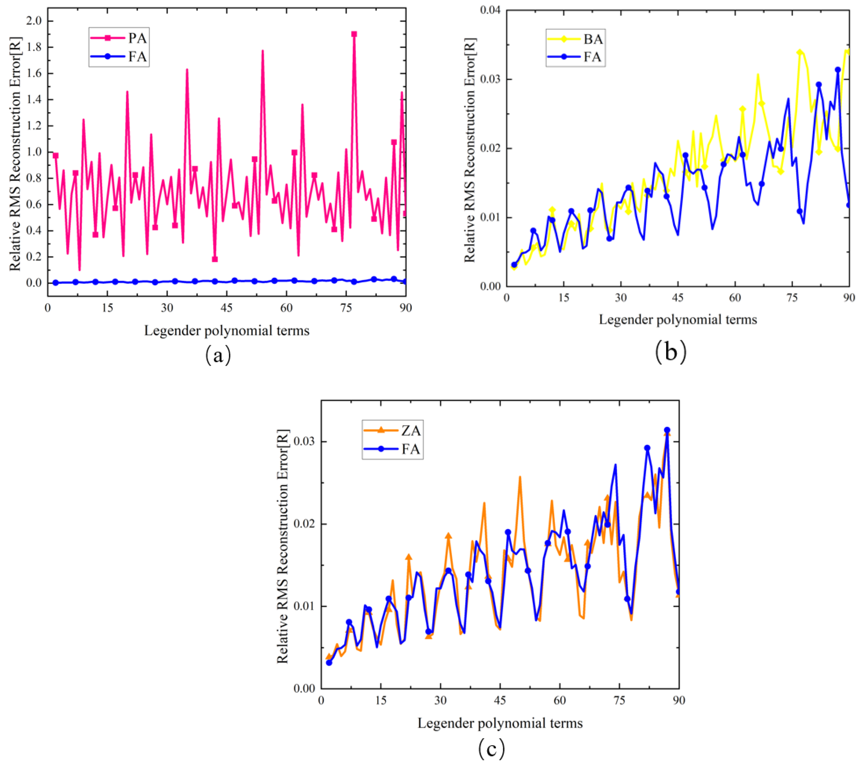
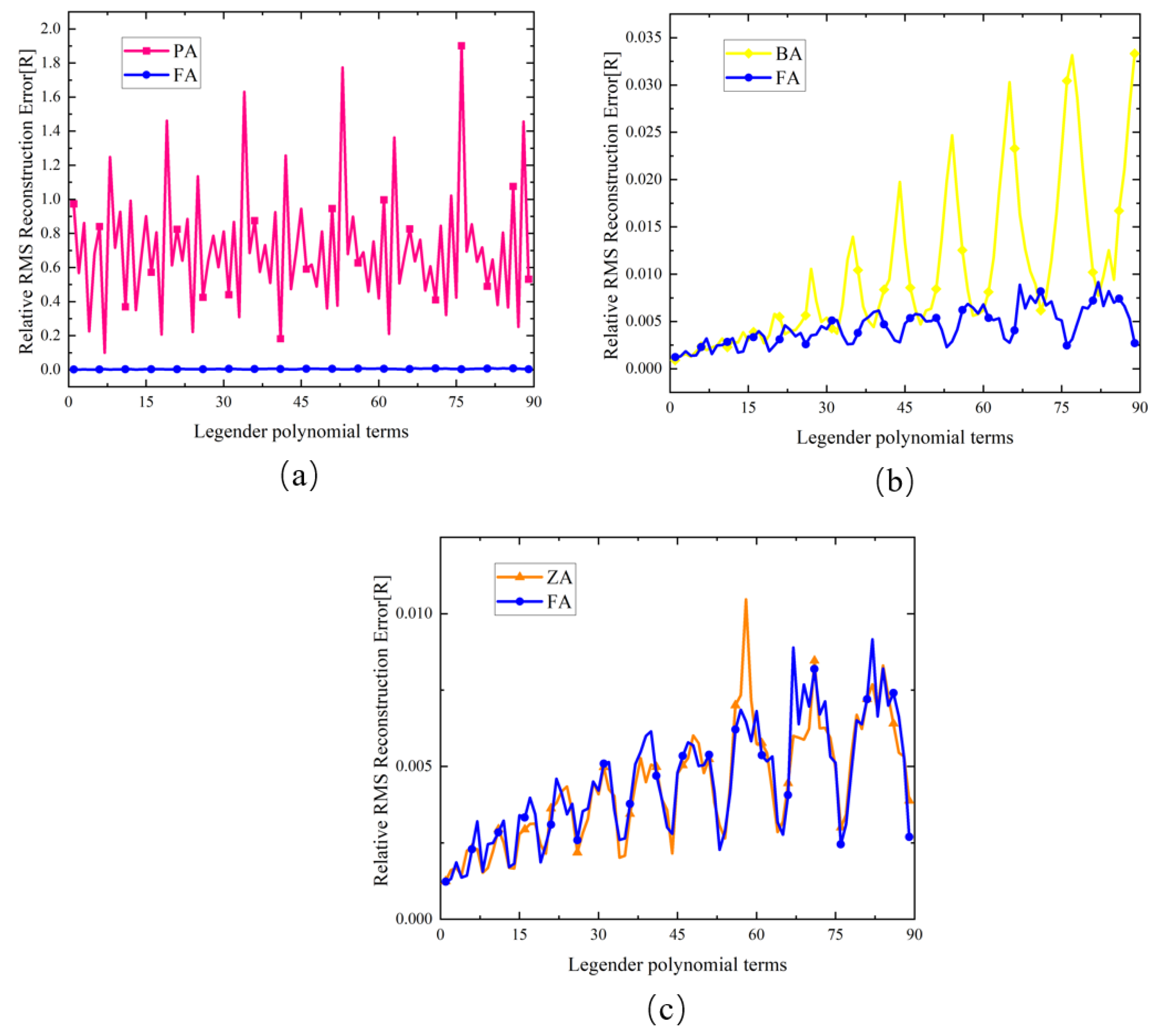
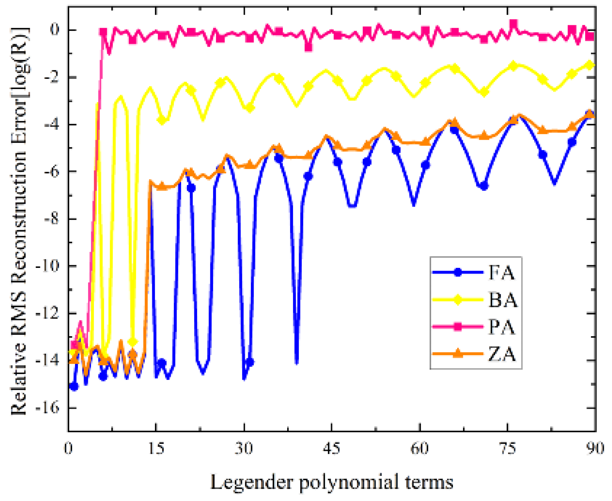
3.1. Algorithm Accuracy

This section focuses on comparing the reconstruction error of the different algorithms in the absence of noise. Legendre polynomials are a complete set of orthogonal polynomials that describe a rectangular surface. The first to the 90th Legendre polynomials are used as the basis functions to simulate the wavefront. In each simulation process, the simulated wavefront is represented by only one Legendre polynomial with a coefficient of 1. The reconstruction range of the entire region is a square region with dimensions ranging from 1 to 1 mm in the x and y dimensions, discretized into a 100 × 100 sub-aperture grid. The reconstructed wavefront W contains the following reconstruction errors:

$$\begin{array}{c}\hfill \mathsf{\Delta }W=W-W_0,\end{array}$$

(15)

where W₀ is the ideal wavefront value. The relative root-mean-square reconstruction error R is applied to evaluate the algorithm error. R is defined as

$$\begin{array}{c}\hfill R=\sqrt{\frac{\mathsf{\Delta }{W}^2}{{W_0}^2}}.\end{array}$$

(16)

Figure 5 shows a comparison of the reconstruction errors between the proposed method (FA) and traditional wavefront reconstruction methods (PA, BA, ZA) without considering noise. Due to the relatively simple surface shape represented by the first 15 terms of the Legendre polynomial expansion, the three improved algorithms (FA, BA, ZA) have similar relative reconstruction errors R. However, beyond the 15th term, the FA, based on truncated Taylor expansion, has a smaller truncation error, resulting in higher reconstruction accuracy. From the simulation results, it can be seen that, compared with existing hybrid reconstruction methods or the multi-directional reconstruction algorithm (BA), the relative reconstruction error value R of the proposed subregion multi-directional slope and curvature mixed wavefront reconstruction method (FA) is reduced by about 4 orders of magnitude. Compared with the ZA, it also has significant advantages in accuracy for certain types of reconstructed surfaces, and the reconstruction accuracy for other surface types is at least comparable to that of the existing algorithms.

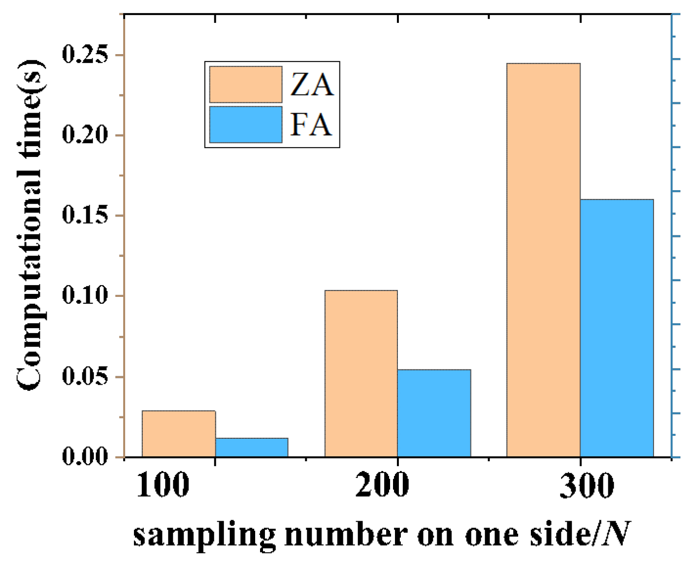
3.2. Reconstruction Speed

Real-time performance is a key metric for the application of reconstruction algorithms in practical engineering, and

Table 1. Reconstruction time for different reconstruction algorithms.

LP17	Computational Time (s)
Algorithm	100 × 100	200 × 200	300 × 300
FA	0.02869	0.10363	0.24451
BA	0.05532	0.29948	0.79579
PA	0.04897	0.14419	0.39198
ZA	0.04248	0.19756	0.58311

compares the processing times of the four algorithms (FA, ZA, PA, BA). The number of one-dimensional sampling points is set to 100 and 200 and 300 in turn. Each runtime result is the average of 20 repetitions. A comparison of the reconstruction time between the proposed reconstruction algorithm (FA) and the existing multi-directional slope–curvature hybrid reconstruction algorithm (ZA) for different sample intervals is shown in Figure 6, which shows that the reconstruction time increases with the increase in the sample points. This study reduces the reconstruction time by fifty percent by reducing the number of integration equations while ensuring accuracy as compared to the previous section.

3.3. Noise Immunity of Algorithm

Gaussian noise is introduced to the ideal slope and curvature using the same simulation conditions as described in Section 3.1. This is carried out to compare the relative reconstruction errors of each algorithm when considering the presence of noise. The level of noise is quantified using the signal-to-noise ratio (SNR), which is defined as the ratio of the root mean square (RMS) of the ideal slope or curvature to the RMS of the added noise as follows:

$$\begin{array}{c}\hfill SNR=\sqrt{\frac{{{\nu }_0}^2}{n^2}},\end{array}$$

(17)

where is the ideal slope curvature information, and n is the introduced Gaussian noise that satisfies the analogue noise with mean 0 and variance 1 and satisfies the Gaussian distribution. The reconstructed information is as follows:

$$\begin{array}{c}\hfill \nu ={\nu }_0+n_0/\phantom{n_{0}SNR}SNR.\end{array}$$

(18)

Wavefront reconstruction simulations are performed at signal-to-noise ratios of 10 and 30. The simulation results are repeated 20 times for each algorithm and then averaged to reduce the effect of randomness.

A comparison of the wavefront recovery reconstruction results for a signal-to-noise ratio of 10 considering noise is shown in Figure 7. As can be seen from the simulation results in Figure 7, in the presence of measurement noise, the present method introduces more integral loop points compared to existing algorithms in that there is a smaller relative reconstruction error for higher-order aberrations, as well as a stronger noise immunity. Compared to the PA and BA, the present algorithm introduces more reconstruction information, resulting in better noise immunity, and, compared to the ZA, the noise immunity remains basically the same due to the same amount of information being introduced.

Figure 8 shows the comparison between the wavefront recovery reconstruction results of the method described in this study and the conventional method when the signal-to-noise ratio is 30, considering noise. From the simulation results of Figure 8, we can see that, as the signal-to-noise ratio increases from 10 to 30, the relative reconstruction errors of the Barwick algorithm and the Pathak algorithm do not change significantly, while the relative reconstruction errors of this algorithm are significantly reduced and have a strong noise immunity. For the low-order polynomials, the reconstruction surface type is relatively simple, and the reconstruction noise immunity advantage of the FA over the BA and PA is not obvious, and several methods have good reconstruction accuracy. As the number of polynomial terms increases, the reconstructed surface pattern becomes complex, and the noise immunity advantage of the FA begins to show. Compared with the ZA, it also has some accuracy advantages in some face shapes.

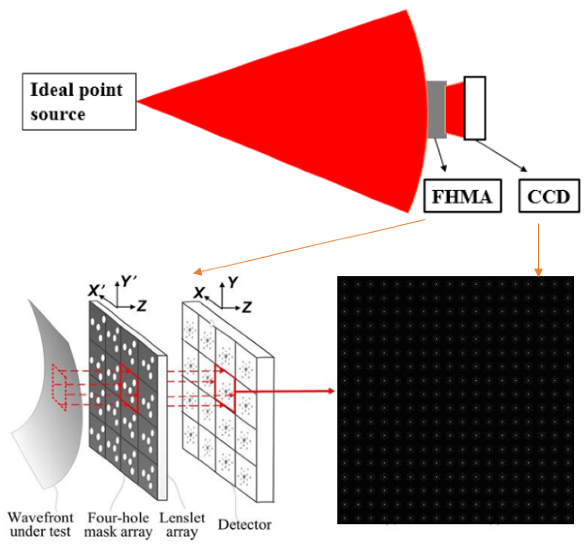
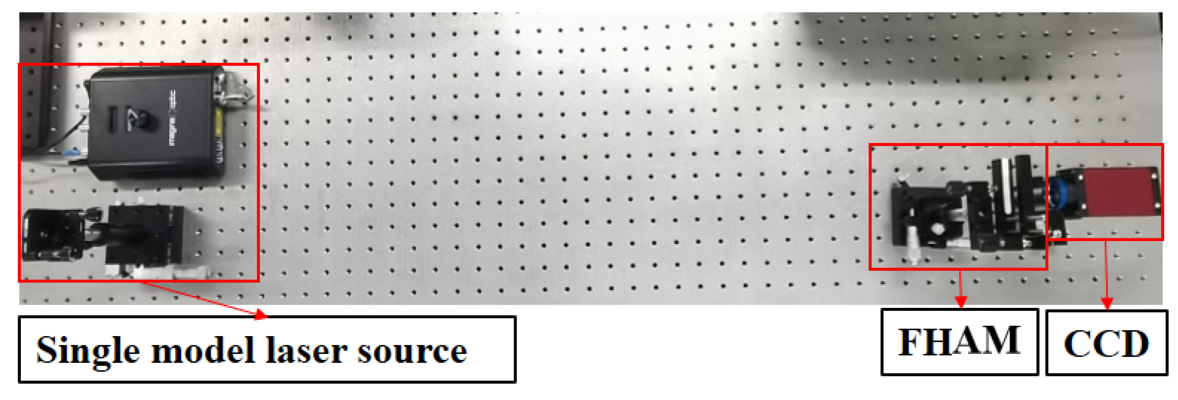
4. Experimental Application

To further substantiate the efficacy and applicability of the algorithm proposed in this paper, this section employs both the ZA and FA methods to reconstruct the collected information from a hybrid wavefront sensor via a null test experiment. The primary objective of this experiment is to ascertain whether the wavefront reconstruction algorithm can accurately recover the known wavefront shape from measured data, particularly under no aberration or ideal wavefront conditions.

This experiment is based on the innovative four-hole amplitude-modulated wavefront sensor (FHAM-WS) [23] proposed by our research group, shown in Figure 9. Building upon the Shack–Hartmann sensor, this sensor modulates the incident wavefront by depositing a chrome layer on the front surface of the microlens array and incorporating four specifically arranged light-transmitting circular apertures within the chrome layer corresponding to each sub-aperture. Based on the far-field optical intensity distribution, the structure can simultaneously measure slope information and curvature information through scalar diffraction theory. This technology utilizes the collection of focal plane spot arrays for wavefront detection, and it has advantages such as a large dynamic range. It holds broad prospects for applications in areas such as high-order aberration measurement.

The specific experimental procedure is as follows. As shown in Figure 10, a single-mode laser source with wavelength of 635 nm is used to generate an approximately ideal spherical wave, and the FHAM-WS, composed of a microlens array and CCD, is placed 1 m away from the light source, which can be considered as an ideal plane wave incident, and the light spot diagram is collected. In this case, the true value of the measurement result of FHAM-WS should be zero, and the closer the actual measurement result is to zero, the smaller the measurement error. Firstly, the slope and curvature extraction algorithm of our research group is used to obtain the complete slope and curvature information of each sub-aperture from the spot pattern. After obtaining the complete mixed data of slope and curvature, the extracted data are processed twice to obtain the slope and curvature data matrix, which is suitable for wavefront reconstruction. Finally, the measured wavefront is reconstructed by using the hybrid slope and curvature algorithm. The experiment reduces random errors by averaging multiple measurements. Focal plane spot arrays are collected every minute, and this process is repeated 10 times. The ideal wavefront slope and curvature information matrices extracted by the experimental setup are reconstructed using the ZA and FA.

The reconstruction results of 10 groups of FHAM-WS measurements produced by the two algorithms are shown in Figure 11. In terms of reconstruction accuracy, the FA algorithm maintains consistency with established, mature algorithms. This is attributable to the simple structure of the reconstructed wavefront under null test conditions. As the complexity of the waveform increases, the precision advantages of the FA algorithm become progressively apparent. Regarding reconstruction time, the FA algorithm exhibits a significant advantage over existing hybrid slope–curvature algorithms. Moreover, the average reconstructed wavefront of the 10 repeated measurements produced using the FA algorithm is shown in Figure 11. It is evident that, under the experimental conditions, the proposed FA algorithm can accurately process slope and curvature information to reconstruct the test wavefront, thereby further validating the effectiveness of the algorithm.

5. Conclusions and Discussion

In this paper, we propose a fast slope–curvature hybrid reconstruction algorithm (FA) and compare it with conventional wavefront reconstruction methods. Through simulation experiments, we find that the FA algorithm has higher reconstruction accuracy in the ideal case and stronger noise immunity in the presence of noise. Compared with the traditional slope–curvature hybrid algorithm and the multi-directional slope–curvature hybrid algorithm, the FA algorithm has a significant advantage in reconstruction accuracy. By introducing slope and curvature information in the diagonal, anti-diagonal, horizontal, and vertical directions with smaller truncation errors, the FA algorithm can provide more accurate reconstruction results. Compared with hybrid reconstruction algorithms that directly introduce information about the diagonal direction, the FA algorithm has a significant accuracy advantage for some reconstructed surface types and provides reconstruction accuracy comparable to existing algorithms for other surface types. In addition, when measurement noise exists, the FA algorithm has smaller reconstruction errors and stronger noise immunity compared to conventional algorithms. In the case of higher-order aberrations, the FA algorithm provides more accurate reconstruction results and introduces more integration loop points to reduce the effect of noise. The null test experiment based on the FHAM-WS has verified the effectiveness of the FA algorithm in practical measurements.

In summary, the FA algorithm proposed in this paper provides higher reconstruction accuracy and stronger noise immunity compared to traditional wavefront reconstruction methods. This algorithm is of great practical significance for wavefront reconstruction and other optical imaging applications.

References

1. Wu, X.; Huang, L.; Gu, N.; Tian, H.; Wei, W. Study of a Shack-Hartmann wavefront sensor with adjustable spatial sampling based on spherical reference wave. Opt. Lasers Eng. 2023, 160, 107289. [Google Scholar] [CrossRef]
2. Valdivieso-González, L.; Muñoz-Potosi, A.; Tepichin-Rodriguez, E. Design and characterization of a safe Shack–Hartmann type aberrometer for making in-vivo measurements: Heuristic approximation. Opt. Commun. 2020, 454, 124500. [Google Scholar] [CrossRef]
3. Bolbasova, L.; Gritsuta, A.; Kopylov, E.; Lavrinov, V.; Lukin, V.; Selin, A.; Soin, E. Atmospheric turbulence meter based on a Shack–Hartmann wavefront sensor. J. Opt. Technol. 2019, 86, 426–430. [Google Scholar] [CrossRef]
4. Birzhandi, S.; Madanipour, K.; Ghanbari, S. Nonlinear refractive index measurement of a trapped particle with Shack–Hartmann wavefront sensor. Opt. Commun. 2019, 444, 154–159. [Google Scholar] [CrossRef]
5. Furukawa, Y.; Takaie, Y.; Maeda, Y.; Ohsaki, Y.; Takeuchi, S.; Hasegawa, M. Development of one-shot aspheric measurement system with a Shack–Hartmann sensor. Appl. Opt. 2016, 55, 8138–8144. [Google Scholar] [CrossRef]
6. Sheldakova, J.; Kudryashov, A.; Zavalova, V.; Romanov, P. Shack-Hartmann wavefront sensor versus Fizeau interferometer for laser beam measurements. SPIE 2009, 7194, 66–73. [Google Scholar]
7. Basavaraju, R.M.; Akondi, V.; Weddell, S.J.; Budihal, R.P. Myopic aberrations: Simulation based comparison of curvature and Hartmann Shack wavefront sensors. Opt. Commun. 2014, 312, 23–30. [Google Scholar] [CrossRef]
8. Zhang, Y.; Wang, S.; Xian, H.; Rao, C. Analytical calibration of slope response of Zernike modes in a Shack–Hartmann wavefront sensor based on matrix product. Opt. Lett. 2022, 47, 1466–1469. [Google Scholar] [CrossRef] [PubMed]
9. Liang, Y.; Zhu, T.; Du, X.; Xu, J.; Fan, S.; Wang, H. Fabrication of a microlens array on diamond for Shack-Hartmann sensor. Diam. Relat. Mater. 2022, 121, 108783. [Google Scholar]
10. Huang, J.; Yao, L.; Wu, S.; Wang, G. Wavefront Reconstruction of Shack-Hartmann with Under-Sampling of Sub-Apertures. Photonics 2023, 10, 65. [Google Scholar] [CrossRef]
11. Mehrabkhani, S.; Wefelnberg, L.; Schneider, T. Fourier-based solving approach for the transport-of-intensity equation with reduced restrictions. Opt. Express 2018, 26, 11458–11470. [Google Scholar] [CrossRef] [PubMed]
12. Li, J.; Xu, J.; Zhong, L.; Zhang, Q.; Wang, H.; Tian, J.; Lu, X. An orthogonal direction iterative algorithm of the transport-of-intensity equation. Opt. Lasers Eng. 2019, 120, 6–12. [Google Scholar] [CrossRef]
13. Nielsen, C.J.G.; Preumont, A. Adaptive Petal Reflector: In-Lab Software Configurable Optical Testing System Metrology and Modal Wavefront Reconstruction. Sensors 2023, 23, 7316. [Google Scholar] [CrossRef] [PubMed]
14. Li, M.; Li, D.; Zhang, C.; Kewei, E.; Hong, Z.; Li, C. Improved zonal wavefront reconstruction algorithm for Hartmann type test with arbitrary grid patterns. In Proceedings of the 2015 International Conference on Optical Instruments and Technology: Optoelectronic Measurement Technology and Systems, Beijing, China, 17–19 May 2015; SPIE: Bellingham, DC, USA, 2015; Volume 9623, pp. 343–351. [Google Scholar]
15. Southwell, W.H. Wave-front estimation from wave-front slope measurements. J. Opt. Soc. Am. 1980, 70, 998–1006. [Google Scholar] [CrossRef]
16. Hudgin, R.H. Wave-front reconstruction for compensated imaging. J. Opt. Soc. Am. 1977, 67, 375–378. [Google Scholar] [CrossRef]
17. Fried, D.L. Least-square fitting a wave-front distortion estimate to an array of phase-difference measurements. J. Opt. Soc. Am. 1977, 67, 370–375. [Google Scholar] [CrossRef]
18. Li, G.; Li, Y.; Liu, K.; Ma, X.; Wang, H. Improving wavefront reconstruction accuracy by using integration equations with higher-order truncation errors in the Southwell geometry. J. Opt. Soc. Am. A 2013, 30, 1448–1459. [Google Scholar] [CrossRef] [PubMed]
19. Viegers, M.; Brunner, E.; Soloviev, O.; De Visser, C.; Verhaegen, M. Nonlinear spline wavefront reconstruction through moment-based Shack-Hartmann sensor measurements. Opt. Express 2017, 25, 11514–11529. [Google Scholar] [CrossRef]
20. Barwick, S. Least-squares estimation for hybrid curvature wavefront sensors. Opt. Commun. 2011, 284, 2099–2108. [Google Scholar] [CrossRef]
21. Pathak, B.; Boruah, B.R. Improved wavefront reconstruction algorithm for Shack–Hartmann type wavefront sensors. J. Opt. 2014, 16, 055403. [Google Scholar] [CrossRef]
22. Zhong, H.; Li, Y.; Qin, P.; He, F.; Liu, K. Hybrid wavefront reconstruction from multi-directional slope and full curvature measurements using integral equations with higher-order truncation errors for wavefront sensors. Opt. Lasers Eng. 2022, 154, 106991. [Google Scholar] [CrossRef]
23. Liu, K.; Wang, X.; Li, Y. Local slope and curvature tests via wavefront modulations in the Shack–Hartmann sensor. IEEE Photonics Technol. Lett. 2017, 29, 842–845. [Google Scholar] [CrossRef]
Figure 1. Geometric schematic of the Southwell model.
Applsci 14 03476 g001
Figure 4. Schematic diagram of residual error analysis: (a) Zhong’s algorithm, (b) the proposed algorithm.
Applsci 14 03476 g004
Figure 5. Comparison of relative reconstruction errors among methods for 1–90th term Legendre polynomials in the ideal case.
Applsci 14 03476 g005
Figure 6. Plot of speed of slope–curvature hybrid reconstruction algorithms.
Applsci 14 03476 g006
Figure 7. Comparison of the reconstruction error of each reconstruction algorithm for a signal-to-noise ratio (SNR) of 10: (a) PA and FA, (b) BA and FA, (c) ZA and FA.
Applsci 14 03476 g007
Figure 8. Comparison of the reconstruction error of each reconstruction algorithm for a signal-to-noise ratio (SNR) of 30: (a) PA and FA, (b) BA and FA, (c) ZA and FA.
Applsci 14 03476 g008
Figure 9. Schematic diagram of the null test experiment using FHAM-WS.
Applsci 14 03476 g009
Figure 10. Experimental setup of the null test experiment using FHAM-WS.
Applsci 14 03476 g010
Figure 11. The reconstruction results of 10 groups of FHAM-WS measurements produced by the two algorithms: (a) reconstruction accuracy, (b) reconstruction time, (c) reconstructed wavefronts under FA algorithm.
Applsci 14 03476 g011