Online Model Adaption for Energy Management in Fuel Cell Electric Vehicles (FCEVs)

Abstract

The growing interest in low-impact mobility technologies has elevated the significance of fuel cell electric vehicles (FCEVs) in the automotive sector. Given the complexity of the resulting powertrain, the need for an effective energy management strategy (EMS) becomes essential to optimize efficiency and energy consumption in vehicles with diverse energy sources. Model-based control is the main approach to address the EMS in electrified vehicles. In particular, fuel cell power is commonly represented through a 1D look-up table using the current demand as input to simplify the implementation in a vehicle control unit. Uncertainties that may be implemented in maps due to simplifying hypotheses, dynamics, ageing, etc., can be propagated to powertrain control, motivating the adoption of adaptive look-up tables for FC modelling. In this study, an extended Kalman filter (EKF) is proposed to adapt the look-up table to actual FC behaviour by measuring its power and gradually correcting calibration errors, drift, and ageing. Subsequently, a standard equivalent consumption minimization strategy (ECMS) is employed to control the FCEV. The fuel cell model is calibrated with experimental data from an FCEV. The results demonstrate that the adaptive strategy outperforms the base calibration. Following an extensive simulation campaign, an improvement of 1.1% in fuel consumption was observed. Remarkably, after just one hour of operation, there was a notable 85% reduction in fuel cell power estimation error, even when the EMS was initially fed a biased look-up table.

1. Introduction

The transport sector represents almost a quarter of Europe’s greenhouse gas emissions and is the main cause of air pollution in cities. Facing this problem, the European Commission (EU) established a series of legislative proposals to decrease the total emissions of the transport fleet, with the final purpose of achieving climate neutrality in the EU by 2050. To carry out this transition, the EU defined an intermediate target of an at least 55% net reduction in greenhouse gas emissions by 2030 [1]. Considering that petroleum-based fuels used in internal combustion engines (ICEs), which are extensively used in vehicle propulsion, are a key actor in the problem of greenhouse gases and air pollution [2], several technologies to progressively replace them are currently on the market. One possibility is the use of hydrogen-based and carbon-neutral fuels [3] to retain the technological knowledge and productive infrastructure of almost a century of ICE development. Another option is the use of battery electric vehicles (BEVs) and hybrid electric vehicles (HEVs).

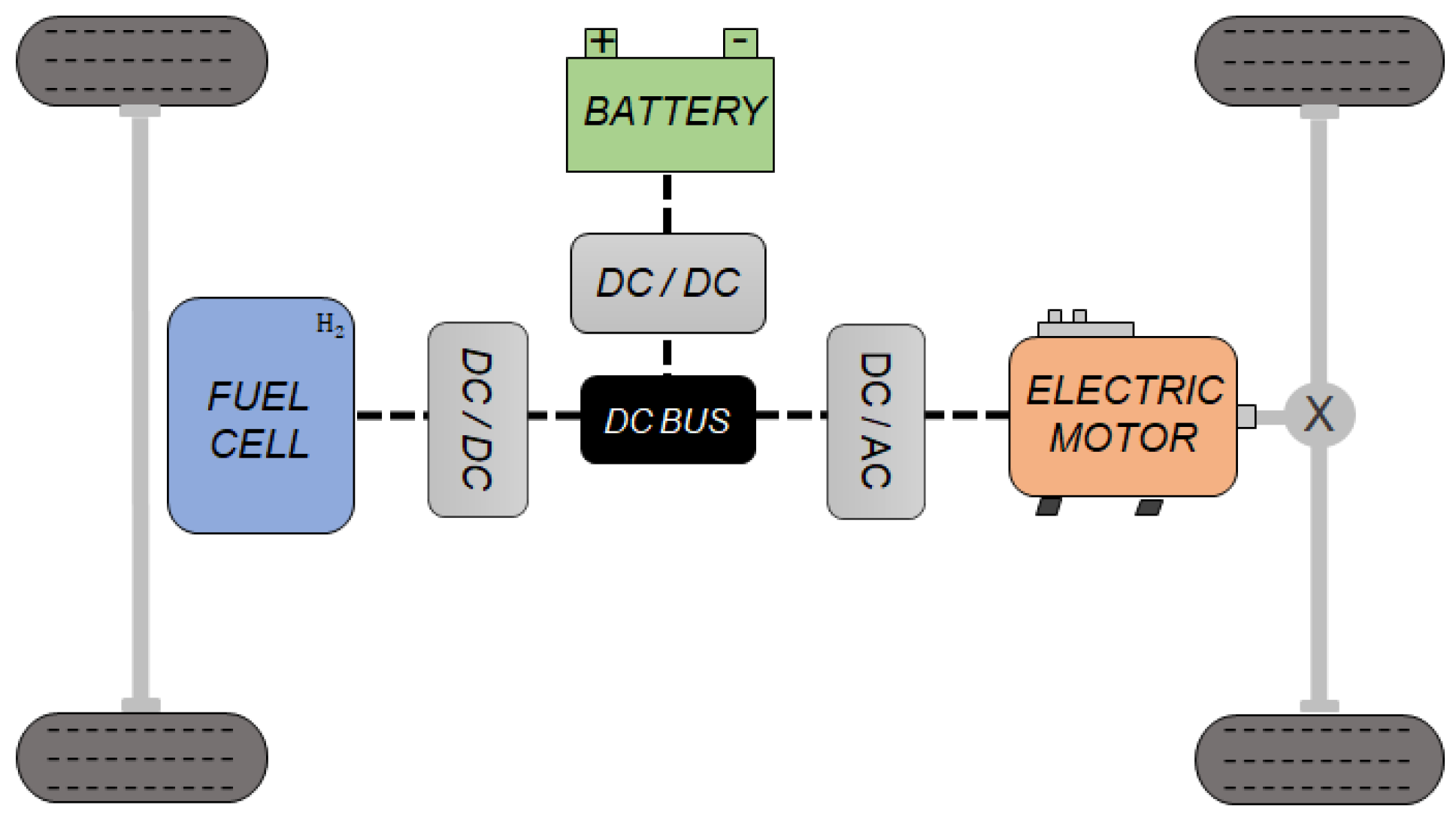
Different types of HEV architectures are designed to accommodate diverse driving needs, efficiency requirements, and technological advancements, and this subject has been widely discussed in the literature [4,5]. A fuel cell electric vehicle (FCEV) is essentially an electric vehicle that combines batteries with a fuel cell to power its onboard electric motor [6]. The fuel cell converts chemical into electrical energy without going through other energy forms such as thermal and mechanical. Therefore, the efficiency of the fuel cell is not limited by Carnot’s cycle, and an FCEV can reach triple the fuel efficiency of a regular gasoline-powered car in some operating conditions [7]. However, fuel cells (FCs) have some drawbacks, such as limited range due to difficulties with hydrogen storage onboard, lack of a hydrogen recharging infrastructure, and safety challenges [8]. So these limitations and system complexity add cost to the production and use of this technology. On the other hand, the source of hydrogen production is an important factor that needs to be considered when defining hydrogen as clean energy. In this sense, when hydrogen is produced by electrolysis using photovoltaic, wind power, or hydraulic power as the source of energy, it is known as green hydrogen [9]. Nevertheless, 95% of the total current worldwide hydrogen production comes from fossil sources and just 4% from electricity [10].

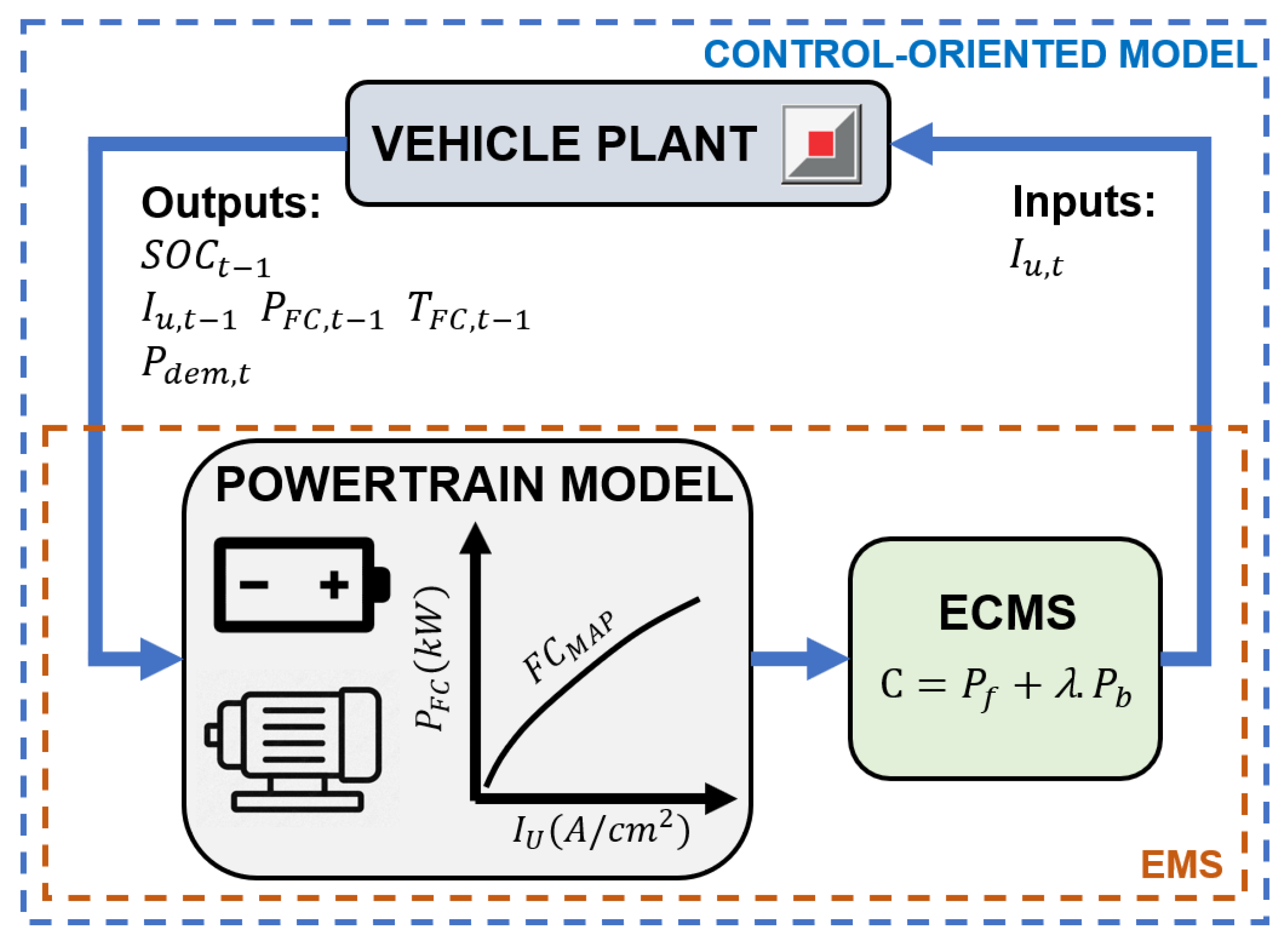
Given the complexity of FCEV powertrains, specifically due to the multiple energy storage systems, the energy management strategy (EMS) is essential for their efficiency and energy consumption [11]. For each situation, the EMS decides the percentage of the vehicle power demand that must be supplied by each of the energy sources [12]. Also, to make this propulsion system competitive and economically viable compared to traditional ICEs, there are still many challenges, such as high maintenance costs and short lifecycle [13]. These challenges are related to the interaction between several ageing mechanisms that react differently with various operating conditions that cause a drop in system performance. The ageing process in fuel cell components also affects the operation of the EMS; however, this aspect is barely considered in the FCEV EMS [14].

Due to the simplicity required for real-time applications, models used for powertrain control are susceptible to uncertainties due to several factors, such as modelling simplifications, limitations in the range of situations considered during calibration, dynamic changes, measurement errors, unit-to-unit variability, or ageing. These errors are propagated to the powertrain control, ultimately impacting the overall performance of the vehicle. In vehicle control applications, electronic control units (ECUs), crucial components in commercial vehicle applications, manage various functions such as engine management, transmission control, and braking systems. ECUs continuously monitor parameters based on sensor inputs to optimize performance, contributing to the overall functioning of the vehicle powertrain [15]. The predominant approach implemented in EMSs and commercial ECUs to model nonlinear and operating-point-dependent behaviours is the use of look-up tables because, even though they require substantial calibration efforts, this is a well-established process in the automotive industry that produces robust performance [16].

The ageing processes in FCs may lead to important differences between the map included in the calibration and that representing the actual fuel cell behaviour. These deviations increase the fuel consumption because the EMS employs a calibration that does not correspond to the actual system state. As a result, these deviations encourage the implementation of techniques that are able to adapt the previously calibrated look-up tables. In this line, ref. [17] proposed a method based on the Lyapunov adaptation law to estimate the linear and nonlinear parameters such as voltage, power, and internal resistance of a polymer electrolyte membrane fuel cell (PEMFC). Also, ref. [18] developed an extended Kalman filter approach for PEMFC to obtain robust real-time-capable state estimations of a high-order FC model for observer applications mixed with control or fault detection.

The use of Kalman-filter-based approaches for state estimation in automotive control strategies has been extensively used, as in [19,20,21,22]. In addition, the Kalman filter can be used for model parameter estimation and, specifically, look-up table adaption. In this context, ref. [16] developed an online adaptive algorithm for NOx map calibration and updating for ICE control based on a simplification of the Kalman filter that allows consideration of updates of the table elements around the measured values instead of the complete table. This proposed solution showed results with similar accuracy to a standard Kalman filter but required lower computational time and memory. In the same field of ICE control, ref. [23] developed a method for bias compensation and online adaption of the air mass flow map of a diesel engine using an extended Kalman filter. As an example of an application in the field of electric vehicles, ref. [24] proposed a method wherein a Kalman filter is used to estimate the ohmic resistance of a lithium-ion battery by updating an entire look-up table based on local estimation at the current operating conditions; the results of the simulations show that the method is able to update the look-up table, even in operating conditions that were barely excited.

In line with the previous discussion, this paper introduces an adaptive approach to enhance calibration of the fuel cell model utilized within the EMSs of FCEVs. The primary aim is to enhance the accuracy of the fuel cell model, consequently improving the overall energy management performance. While existing research utilizes observers to estimate the internal states of fuel cells for vehicle control applications [25,26] or to approximate look-up table parameters in conventional ICE vehicles [16,23], this work brings the novelty of developing an adaptive strategy for online map calibration and updating fuel cell models implemented in the EMS of an FCEV. In this way, the paper analyses the potential of updating the FC model by an extended Kalman filter (EKF) used in the EMS, highlighting the effect of the improved accuracy with respect to fuel consumption. These parameters are adjusted based on FC power measurements using an EKF approach. The EMS maintains a simple look-up table but with improved performance by correcting calibration errors, drift, or ageing.

The article is structured as follows: In Section 2, ’Methodology’, we introduce a case study, describe the fuel cell model calibration process, provide details about the vehicle model, and discuss the energy management strategy along with the proposed approach. Following this, the results are discussed in Section 3, where the baseline calibration is compared with the proposed approach, and the algorithm adaptation speed is also investigated. The final conclusions of the article are presented in Section 4.

2. Methodology

2.1. Case Study

The paper focuses on online adjustments to the model to relate the fuel cell current and power in the EMS of an FCEV. This adaptation improves the system control by preventing errors that may propagate to the powertrain caused by the FC system ageing process and drift. In this sense, the plant considered is the FCEV for which the architecture is shown in Figure 1 and for which the main parameters are included in

Table 1. Description of the FCEV’s main features.

Parameter	Value
Weight	1814 kg
Frontal area	2.73 m2
Motor power	120 kW
Battery capacity	1.5 kWh
Battery voltage	230 V
FC rated power	95 kW

Hyundai Nexo specifications.

. To represent the power-split between the battery and the fuel cell, a control-oriented model (COM) is built, for which the complete FCEV model built in the v2020 GT-Power software is used as a vehicle plant. GT-Power is a performance simulation software extensively utilized by leading vehicle manufacturers for vehicle modelling. This versatile tool enables the design and analysis of diverse powertrain topologies, encompassing internal combustion engines, hybrid electric systems, and fuel cell vehicles [27]. With GT-Power, engineers can assess crucial performance metrics such as power output, fuel efficiency, emissions levels, and thermal management. Its comprehensive capabilities make it an invaluable resource for optimizing vehicle design and performance across a wide range of applications in the automotive industry. The GT-Power FC model was calibrated with experimental data, and the FC maps employed in the EMS were obtained through steady-state simulation, as described in Section 2.3.

In order to evaluate the impact of the 1D table accuracy employed in the EMS, three different scenarios are assessed. The first case considers perfect knowledge of the FC state. In this scenario, the GT model is used extensively to create a 1D look-up table relating the FC current with its power, corresponding to the map calibrated by testing the FC in steady-state conditions, represented in Figure 2 as Actual map (AM). In a second scenario, the Biased map (BM) of the FC is considered as the reference. This case aims to estimate the impact of errors in the FC map used for control purposes in the ECMS: a situation that becomes more important as the FC ages and presents a significant performance drop due to the degradation process. This represents the condition where the brand-new FC calibration remains constant for the entire FCEV’s useful lifespan.

To rectify errors that may propagate to the powertrain control due to biased maps, the third case proposes a strategy that involves progressive updating of the BM and eventually improving the results obtained with the FC map obtained by the AM, since the adaption is able to capture, to some extent, the FC dynamics that were not considered in the original scenario. Figure 3 illustrates the driving cycles recorded by a passenger car during its daily journeys, encompassing a wide range of driving conditions, including highway travel and urban routes with varying traffic densities and traffic signals, encompassing a range of driving conditions commonly encountered by vehicles in real-world driving scenarios. These driving cycles are employed in the simulation to evaluate EMS performance considering the three different maps. However, it is important to note that while these daily trajectories represent a specific route, the driving profiles are subject to variations influenced by driver decisions and the actual traffic conditions, resulting in fluctuations in total travel time.

2.2. Experimental Setup

In order to build a high-fidelity vehicle model in GT-Power, an experimental study was conducted by employing a fuel cell light duty vehicle, the main characteristics of which are listed in Table 1, mounted on a chassis dynamometer test. The testing campaign was done using a dynamic vehicle test bench boasting a continuous power output of 120 kW and a continuous torque of 1100 Nm. To capture critical data, an on-board diagnostics (OBD) interface was employed to measure electrical current and voltage within the FC and to monitor the battery voltage, while the battery current was measured using a current clamp. This experimental setup facilitated the acquisition of the polarization curve for the FC. During the tests, the ambient air was not controlled due to test bench limitations, which naturally fluctuated between 24 and 29 °C. The experimental conditions involved maintaining the vehicle at constant speeds of 60, 80, and 100 km/h. The accelerator signal was systematically adjusted in steps, ranging from maximum to minimum, and each setting was maintained for a duration of 20 s. The polarization curve and the fuel cell output power measured in these conditions are shown as the green curve of Figure 4. The maximum fuel cell output power measured at the test conditions was 81.4 kW.

2.3. Model Description

This study is conducted by modelling an FCEV on GT-Power; a detailed vehicle model is built as a vehicle plant. In the COM, the fuel cell power is modelled as a 1D look-up table using as input the FC current density $I_u$. Figure 5 shows how the COM is organized. The v2021b MATLAB/Simulink interface is where the EMS is implemented. This interface addresses the proposed method of this study and also the standard ECMS applied to control the FCEV. The EMS receives the outputs of different parameters from the vehicle plant from the previous time step, where $SOC$, $I_u$, $P_{FC}$, and $T_{FC}$ represents the battery state of charge, current density, fuel cell power, and fuel cell temperature, respectively. Moreover, the disturbances related to the driving demands at the current time step are taken into consideration, such as $P_{dem}$, which represents the power demanded by the electric motor to drive the vehicle. Then, the ECMS employs the powertrain model to compute the power-split between the battery and the fuel cell to fulfil the power demand based on the ECMS strategy, providing as input only the current density for the vehicle plant according to the output power estimated by the 1D table.

The GT-Power PEMFC template is used to model the FC according to experimental results. The new FC model shown in Figure 4 is calibrated using the experimental polarization curve as input for the model; this curve represents the output power of a brand-new FC model in steady-state conditions. However, hydrogen consumption is not measured by the vehicle test bench, so hardware design specifications are adjusted to match FC efficiency values found on experimental works developed using the same vehicle [28]. Similarly, the maximum and minimum reported efficiencies regarding hydrogen consumption and FC output power are 65% and 45% at minimum and maximum current densities, respectively.

Since the new FC model is calibrated to represent a brand-new FC, this polarization curve was scaled to represent an aged FC close to the end of its lifetime, as shown in the figure. Usually, the failure threshold of a PEMFC is defined as a 10% drop in the voltage performance [29]. So the polarization curve of the new FC model was progressively scaled, reducing the voltage curve by 5% at low- to 10% at high-current densities to represent the aged FC model while maintaining the hardware design and other parameter calibration of the new fuel cell model. Finally, this aged FC model calibration was employed in the FCEV model to evaluate the impact of using a map of a new FC to control an aged one and to develop the proposed adaptive strategy.

This paper assumes that the FCEV employs a battery pack and a fuel cell. Figure 1 shows how the powertrain is built and the electrical connections between its components. The powertrain integrates these components through a DC bus. A DC/DC converter links the fuel cell and battery, while a DC/AC converter connects to the 120 kW electric motor. Considering 95% efficiency for power losses, the study excludes grid charging. The FCEV is modelled with a Li-ion Battery—62 serial cells and 2 in parallel, totalling 1.5 kWh capacity and 230 V voltage. Its equivalent circuit (RC) considers state-of-charge-dependent open-circuit voltage and resistance. The body specifications are those of the Hyundai Nexo [28] for longitudinal vehicle dynamics and power demand computation.

Due to the powertrain architecture considered in the FCEV model, the power demand required by the electric motor to drive the vehicle over the considered driving cycle $P_{dem}$ must be supplied by the net electrical power of the battery $P_{batt}$, output power of the fuel cell $P_{FC}$, or a combination of both, as given by:

$$P_{dem}=P_{batt}+P_{FC}$$

(1)

So $P_{dem}$ depends on the progress and conditions imposed by the driving cycle. Taking $I_u$ as the control variable, $P_{FC}$ is directly estimated based on the FC map. Finally, $P_{batt}$ can be obtained by:

$$P_{batt}=P_{dem}-P_{FC}\left(I_u\right)$$

(2)

The fuel consumption is chosen as the cost to be minimized, although, similarly, the fuel cost, the total energy consumed, or the cost production could be used. Therefore, the problem of the EMS can be defined as finding the powertrain control law $u\left(t\right)$ over a driving condition with a duration of $t_f-t_0$ that minimizes the cost:

$$J={\int }_{t_0}^{t_f}{P}_f\left(u\left(t\right),t\right)\mathrm{d}\mathrm{t}$$

(3)

where $P_f$ is the power of the fuel consumed, and it directly depends on the control variable u, i.e., $I_u$, and it is the single input of the EMS for the FCEV model. As $P_f$ is proportional to hydrogen consumption, minimizing the cost function (Equation (3)) relies on reasonable estimation of the output power that the fuel cell can provide in all driving conditions that the vehicle is exposed to from $t_f-t_0$. Taking into account the explicit relation between $P_{batt}$ and $P_{FC}$, Equation (4) represents the dynamic behaviour of the energy stored in the battery, and $P_b$ is the variation in the battery’s state of energy (considered positive when the battery is being discharged and negative when the battery is being charged):

$${\dot{E}}_b=-P_b$$

(4)

Note that due to the electrical link, $P_b$ can be computed from Equation (1), and it is dependent on $P_{dem}$ and $P_{FC}$. Then, the battery can be discharged by supplying $P_{dem}$ and charged by regenerative braking or electrical power given by the fuel cell.

2.4. Energy Management Strategy

As this vehicle is not a plug-in HEV, the energy that will maintain the vehicle in the charge sustaining mode comes exclusively from the hydrogen consumed by the FC. Moreover, for a fair comparison in terms of general performance and fuel consumption between the different cases in this study, the battery state of charge (SOC) at the end of the driving cycle should be zero to guarantee charge-sustaining operation and to allow fair comparison between the scenarios. Finally, considering these constraints, the problem is defined as:

$${\int }_{t_0}^{t_f}{P}_b(u\left(t\right),E_b\left(t\right),t)d_t=0$$

(5)

So to address the constraint of the charge sustaining mode in the FCEV and the condition for which the driving cycle is not known in advance, the ECMS initially proposed by [30] is implemented in the EMS. The idea underlying the ECMS is to solve the global optimization problem (Equation (5)) by replacing it with a local one, then to reduce the problem to the minimization of the equivalent fuel consumption at each time step. Thus, it is possible to define an instantaneous cost that takes into account both hydrogen and electric energy consumption, such as:

$$C=P_f-\lambda P_b$$

(6)

Note that the $\lambda$ parameter weights (Equation (6)) the power usage to move the vehicle at a given time step. If $\lambda$ tends to 0, the EMS only takes into account the fuel power, tending to deplete the battery. On the other hand, if $\lambda$ tends to ∞, the variation to the SOC is minimized, and high power is provided by the fuel cell. $P_f$ and $P_b$ have the same units, and, consequently, the co-state $\lambda$ is dimensionless. Due to the limitations of obtaining a $\lambda$ that fulfils the constraint of Equation (5) in cases for which the cycle is not known in advance, a controller is implemented in the EMS to manage this task. This controller is based on what [31] proposed in his work. Basically, the controller attribute a correction factor according to the error between the actual SOC and the target SOC. A non-linear penalty function is defined heuristically in order to maintain the SOC around the target value (50%), delimited from 40% to 60%.

2.5. Proposed Method

Recalibrating maps has shown to be useful for control applications to avoid the propagation of errors to the powertrain control caused by bias. So this work proposes an approach that consists of modelling the FC power output power as a 1D look-up table using the FC demanded current as input and for which the parameters are adapted based on FC power measurements using an EKF. The map adaptations take place while the FCEV covers a route, the fuel cell operates, and the learning block presented in Figure 5 evaluates the fuel cell output power measurement and compares it with the mapped output power implemented in the EMS.

The proposed strategy addresses an online adaptation of a 1D look-up table M calibrated with experimental data under steady-state conditions. This table provides the estimated output power of the fuel cell $P_{\mathrm{F}\mathrm{C}}$ based on the input current density $I_u$. The look-up table is composed of an input axis ${\mathbf{I}}_{\mathbf{M}}$ and an interpolated axis ${\mathbf{P}}_{\mathbf{M}}$, both with n elements. The look-up table is defined as follows:

$$P_{FC}=M\left(I_u\right)=\mathbf{q}({\mathbf{I}}_{\mathbf{M}},I_u)·{\mathbf{P}}_{\mathbf{M}}$$

(7)

where $\mathbf{q}$ is a vector of the same size (10 elements), computed by:

$$\mathbf{q}=1-\frac{|I_{u,k}-{\mathbf{I}}_{\mathbf{M}}|}{{\displaystyle \sum _{i=1}^n|I_{u,k}-{\mathbf{I}}_{\mathbf{M}}\left(i\right)|}}$$

(8)

where $I_{u,k}$ is the current density applied, and ${\mathbf{I}}_{\mathbf{M}}$ is the vector of n input values of the table and ranges from 0 to 1.75 A/cm².

Moreover, the output of the table ($P_{\mathrm{F}\mathrm{C}}$) is filtered to reject disturbances on the system and sensor noise as following:

$$P_{FCf,k}=a{P}_{FCf,k-1}+(1-a)P_{FC,k}$$

(9)

where a is the filtering parameter fitted to the simulations and is equal to 0.2. To adapt the look-up table, a Kalman filter is developed to update the table data elements ${\mathbf{P}}_{\mathbf{M}}$. So the main equations of the Kalman filter are recalled to present the mathematical terminology. The following equations will explain the flowchart presented in Figure 6, which depicts the proposed strategy. It is based on a discrete-time system:

$$x_k=F{x}_{k-1}+B{u}_k+w_k$$

(10a)

$$y_k=H{x}_k+v_k$$

(10b)

where the sub-index k is the time step, $x_k$ represents the state vector, $u_k$ is the input vector, and $y_k$ is the output vector. The variables $w_k$ and $v_k$ are the white Gaussian noise terms that induce the variations. F represents the transition matrix, B is the control-input matrix, and H is the observation matrix.

In the case at hand, the output of the system $y_k$ attends to the power measured at the fuel cell $P_{FCf}$, the input $u_k$ corresponds to the intensity at each time step $I_u$, while the state vector $x_k$ comprises all the elements of the table data $P_M^i$ and the estimated power of the fuel cell $P_{FCf}$:

$$x_k=\left[\begin{array}{c}{P}_{M,k}^1\\ P_{M,k}^2\\ \dots \\ P_{M,k}^n\\ P_{FCf,k}\end{array}\right]$$

(11)

The noises $w_k$ and $v_k$ are assumed to be independent and to both have Gaussean distributions with zero means and covariance matrices $Q_k$ and $R_k$.

Note that Q is the identity square matrix of the n length of the 1D look-up table, and ${\tau }_x$ can be selected individually for each table data element containing its individual variances. It is helpful to consider the order of magnitude of the data, i.e., absolute error for high powers may be higher than for low loads. Then, Q is represented by

$$Q=\left[\begin{array}{ccccc}& & & & \\ & & ide{n}_{n+1}& & \\ & & & \end{array}\right]{\tau }_x$$

(12)

and the linearised process matrix is defined by

$$F_k=\left[\begin{array}{cc}\begin{array}{ccccc}& & & & \\ & & ide{n}_n& & \\ & & & \end{array}& 0\\ (1-a)q_k& a\end{array}\right]$$

(13)

In this case, H is constant because q and a are included in the process matrix (Equation (13)). Then, in the prediction step, ${\widehat{x}}_k$ is the observation of the state vector $x_k$

$${\widehat{x}}_{k|k-1}=F_k{\widehat{x}}_{k-1}+B{u}_k$$

(14a)

This assumes no variations to the table elements and estimates the fuel cell power at the current time step. Then, entering the update step, the error between the power estimation and the fuel cell power measurement can be evaluated:

$$e_k=y_k-H{\widehat{x}}_{k|k-1}=P_{FCm,k}-P_{FCf,k}$$

(14b)

Finally, with the error $e_k$ and the Kalman gain $K_k$, it is possible to update the new table data elements of M and obtain the final estimation of power:

$${\widehat{x}}_k={\widehat{x}}_{k|k-1}+K_k{e}_k={\mathbf{P}}_{\mathbf{M}}$$

(14c)

where $K_k$ is the Kalman gain and is solved by the following iterative equation:

$$P_{k|k-1}=(F_k{P}_{k-1}{F}_k^T+Q)$$

(15a)

$$K_k=\frac{P_{k|k-1}{H}^T}{H_k{P}_{k|k-1}{H}^T+R}$$

(15b)

$$P_k=(I-K_k{H}_k)P_{k|k-1}$$

(15c)

where the matrix $P_k$ is the covariance matrix of the state estimate error that will be used in the next time step to estimate the observation of the state vector (Equation (14a)) and the Kalman gain (Equation (15b)).

The noise covariance matrix R is constant and is an essential parameter of the proposed method that governs the algorithm. The learning rate affects how fast the algorithm can adapt the map. Observe that increasing the Kalman gain value assigns greater weight to the error computed by the difference between the measured and the estimated power by the map (Equation (14b)). Then, the new table data elements are updated quickly (Equation (14c)). On the contrary, when applying low learning rates, the new table data elements rely more on the previously implemented data elements. In the results section, we discuss how increasing or decreasing the parameter affects the map adaptations.

Note that although at each time step just a single value is estimated ($P_{FCf,k}$) and compared with the measured FC output power ($P_{FCm,k}$), the elements around the value are also adjusted by multiplying $K_k$ and $e_k$ due to the filter implemented in F (Equation (13)).

3. Results and Discussion

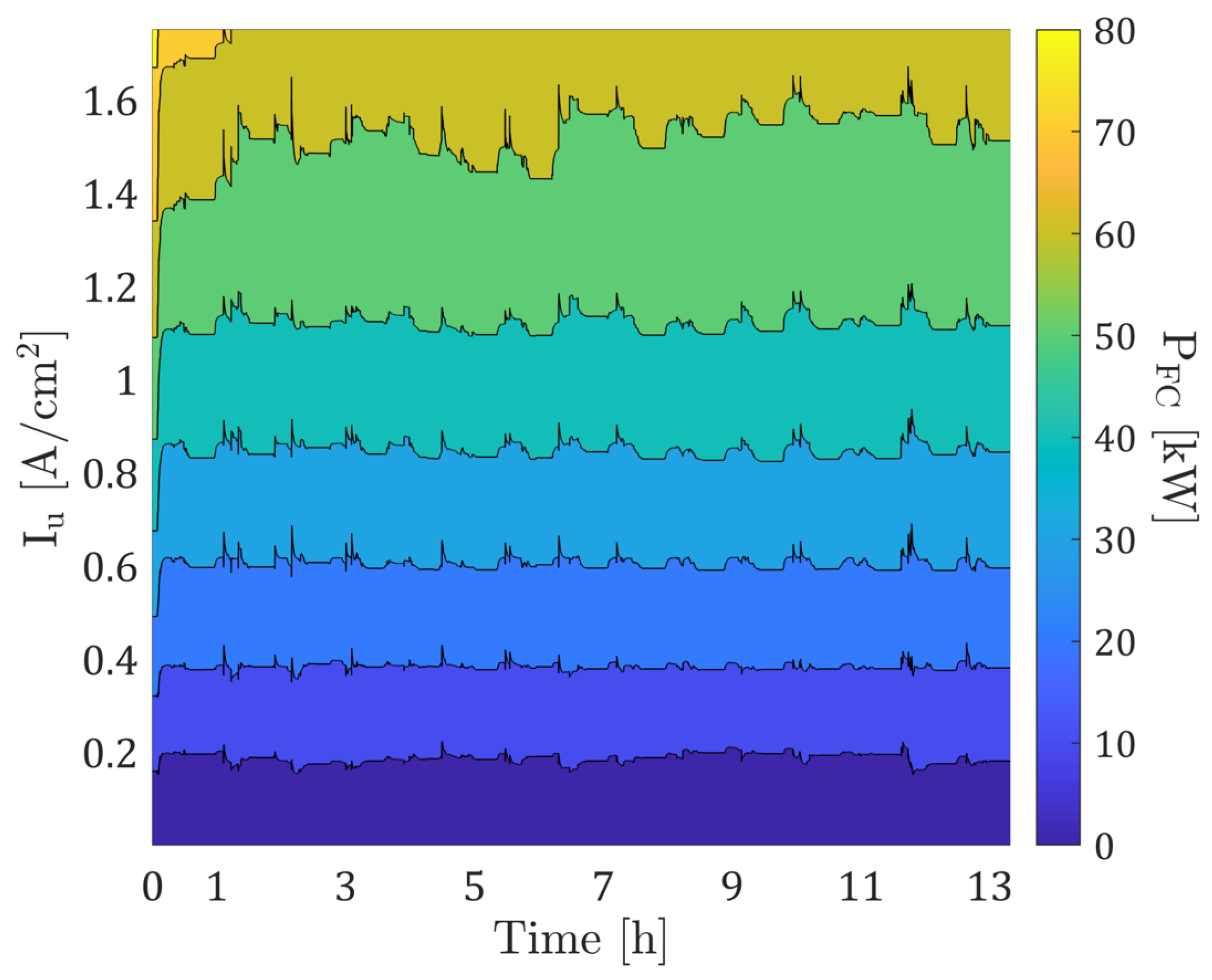
The evolution of the map adaptations by the proposed method when the FCEV is covering 15 cycles is shown in Figure 7. This figure shows how the learning map (LM) evolves as the vehicle covers the different driving conditions of the cycles. To expose the method to the worst scenario, at the start of the test, the map of the BM was conditioned as the initial map. In this case there is no information about the ageing level of the FC or operating time that the FCEV has already covered. Due to the warming and low-temperature conditions of the fuel cell, the adaptations are only activated at temperatures above 340 K to avoid corrections during these short periods. Once the fuel cell starts to run and the correction is activated, the adaptation on the maps evolves, and when the FCEV switches off, the map is stored and then used for the next trip and so on. When the FCEV runs again, the map keeps evolving to correct these deviations.

According to Figure 7, as the time duration of each cycle is around one hour, higher correction rates are observed during the first driving cycle. So in this case, about 1 h is needed for the algorithm to adapt the map and stabilize it until reaching a condition with lower amplitudes in the map adaptation. Furthermore, one can expect that even if the algorithm strongly adjusts the map in the first hour, the map should maintain a relatively stable map profile during subsequent hours, particularly at high current densities. The ongoing variations observed from medium to high current densities are closely linked to the dynamic responses of the fuel cell. This phenomenon is primarily attributed to rapid changes in the fuel cell operating conditions, often resulting in fuel cell stack temperature fluctuations.

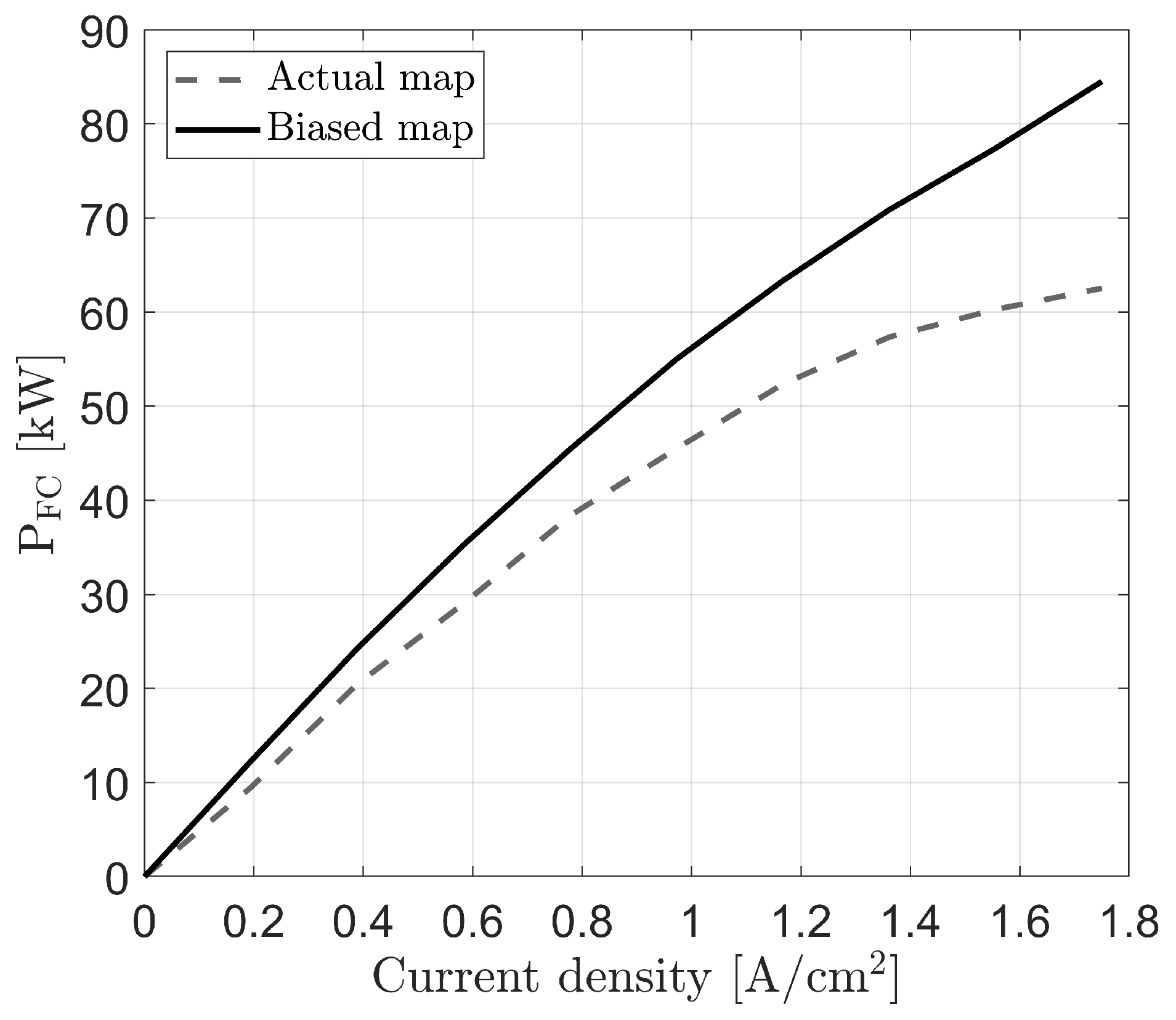
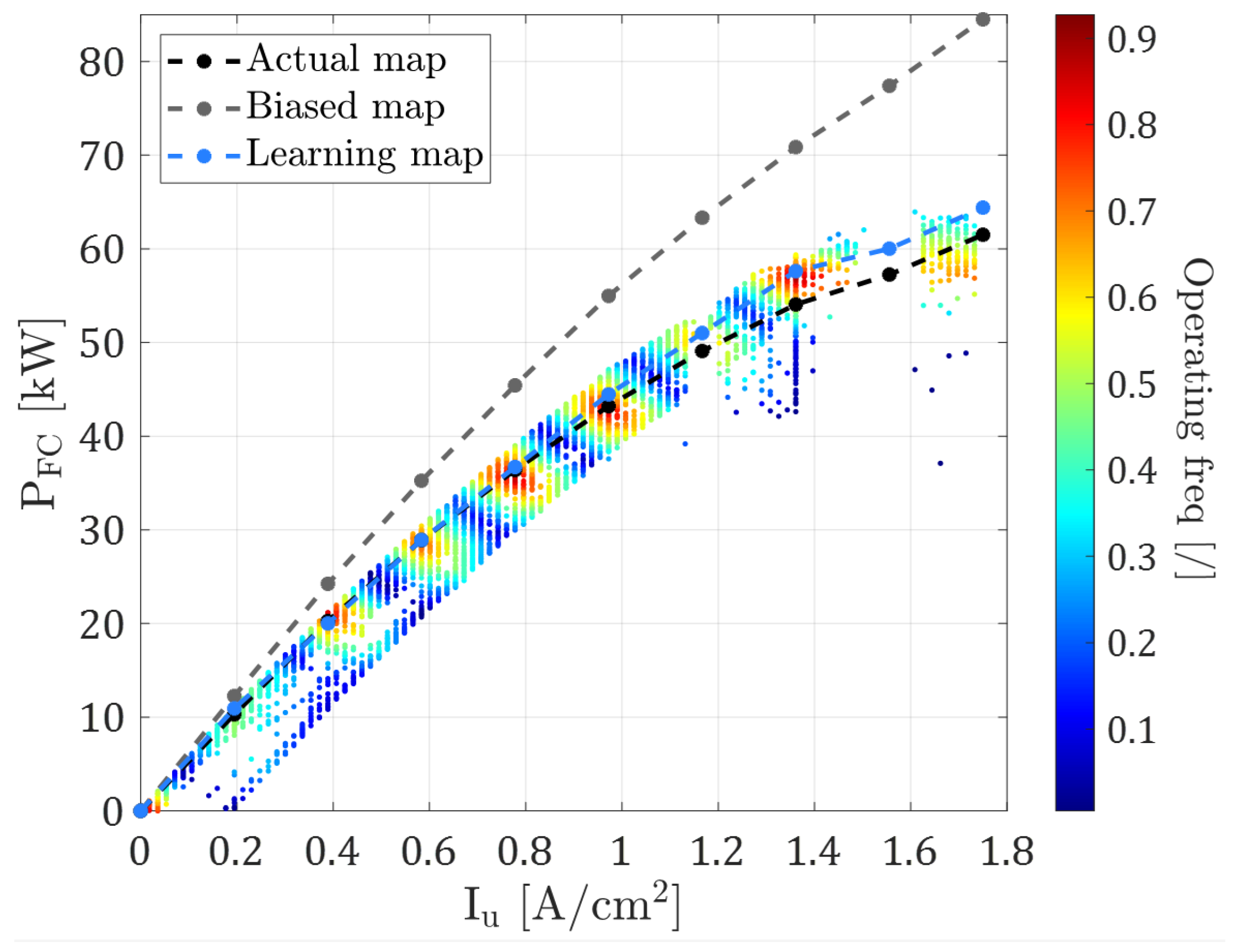
For comparison purposes, Figure 8 illustrates the three maps together. In the cases of the AM and BM, these maps remained constant throughout all simulations. In contrast, for the LM case, this map represents the final adaptation achieved after the end of the simulations. Regarding the operating points distributed on the plot, these points represent the output power of the fuel cell as a function of the control input $I_u$ provided by the EMS to the fuel cell over the 15 cycles of the LM case.

According to Figure 8, two problems can be underlined when working with COM. First, the differences between the full cell power estimated by the COM (1D look-up table) and the one provided by the plant (GT model) depend on the calibration. However, despite the high calibration effort for mapping the fuel cell used in the AM, this map still shows that it is impossible to cover the region perfectly with the highest operating frequency (red), showing that it is possible to correct and improve the accuracy of the FC models. Second, independent of the model calibration, there will always be deviation in the estimation due to simplification of the system to a 1D look-up table. For this reason, providing a more accurate estimation of the output FC power by the EMS can ensure that the FC will operate closer to optimal conditions and then improve fuel consumption. Moreover, as observed in the map adaptations of Figure 7, it is expected that if the adaptative method can provide quick corrections to the map, the difference between the actual output power the FC provides and the one estimated by the map can be minimized. To some extent, the system dynamic can be considered by the EMS to compute the proper power split, which will be further discussed in this section.

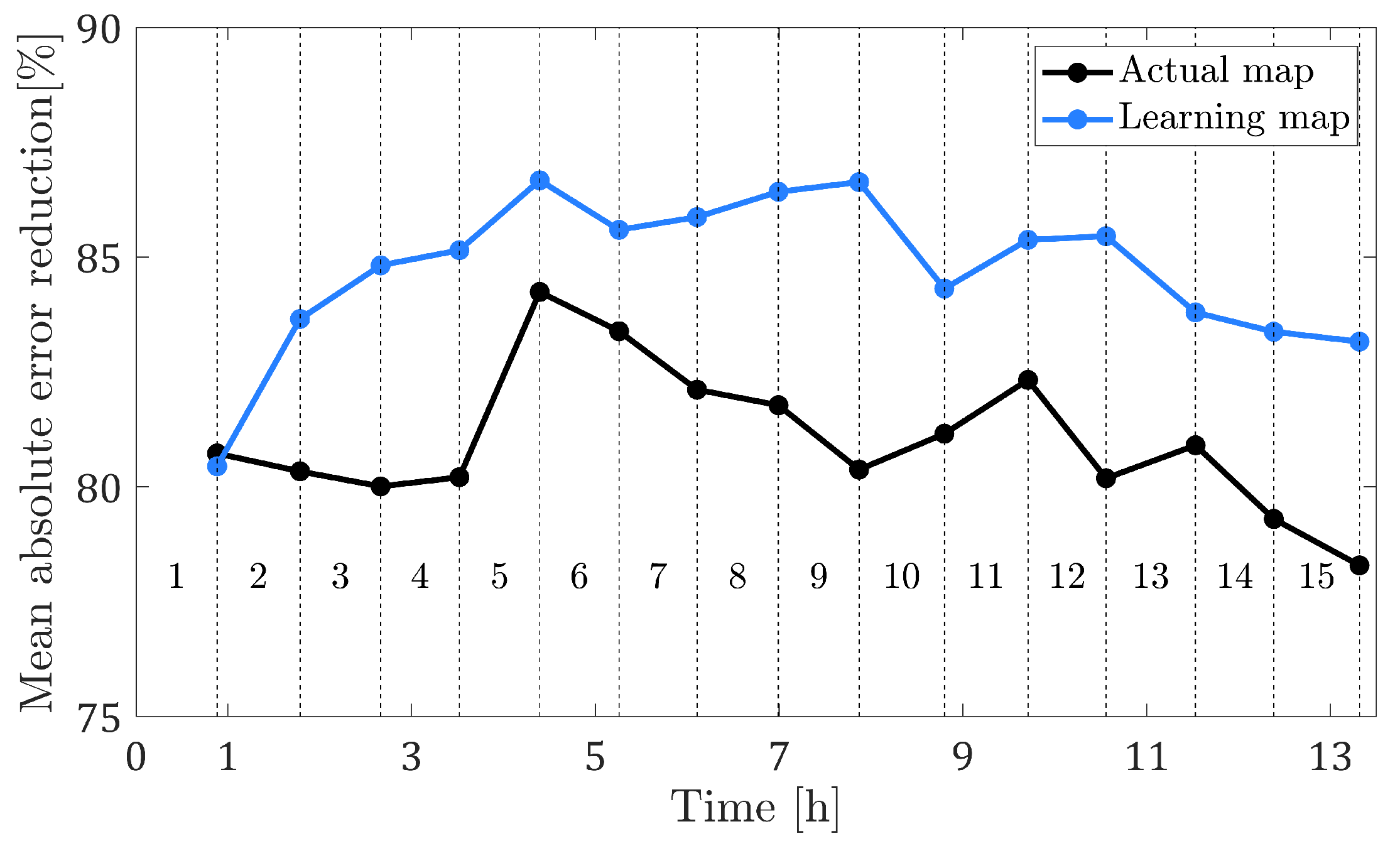
Figure 9 presents the reduction in the mean absolute error (MAE) for fuel cell power estimation in the AM and LM compared to the BM under identical driving conditions. This approach allows a statistical comparison of how the three maps correlate with the actual fuel cell output power. The MAE is calculated by determining the absolute difference between the predicted FC power estimated by the maps and the measured FC output power for all the data in one cycle. Remarkably, within just 1 h of operation, the LM achieves substantially lower estimation errors, obtaining an error reduction of 85% compared with the BM. In contrast, the AM reduces the error by around 81%. These results highlight that the BM does not provide an acceptably accurate estimation of fuel cell power and propagates errors that can affect powertrain control and overall vehicle performance. However, even though the AM achieves a similar error reduction to the LM, it relies on a complex calibration process that maps the aged FC model under steady-state conditions. This calibration process involves substantial effort to determine the actual level of ageing in the fuel cell, making it impractical for real-time control applications, suggesting the need for adaptation algorithms to improve calibration accuracy.

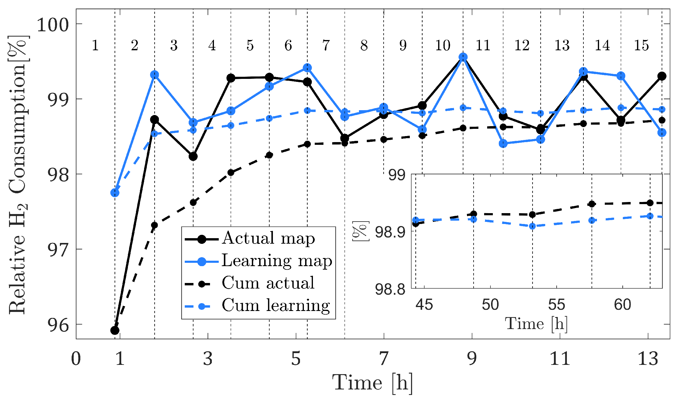
As expected, by increasing the fuel cell power estimation accuracy, the EMS can also generate better control actions for the fuel cell, thus ensuring fuel savings. Moreover, Figure 10 shows the relative ${\mathrm{H}}_2$ consumption compared with that of the BM for each cycle and for the cumulative results of the 15 cycles. Due to the higher estimated error the BM provides, its poor estimation also affects the ${\mathrm{H}}_2$ consumption. When examining the LM, a reduction of 1.6% was observed in cycle 11 compared to the BM reference case, with a cumulative decrease of 1.2% across all cycles. Similarly, the AM exhibited a reduction of close to 1.7% in cycle 3 and a reduction of 1.3% for the cumulative consumption. It is important to note that the initial fuel consumption difference in the first cycle is influenced by variations in the battery state of charge that each of the three cycles reaches at the end of the cycle. In this context, AM significantly reduced hydrogen consumption due to higher battery energy depletion. However, considering long-term vehicle operation, it is possible to observe that after 45 h of vehicle use, the battery state of charge variation tends to be minimized, and the LM can overcome the cumulated ${\mathrm{H}}_2$ consumption and start to save fuel compared to the AM.

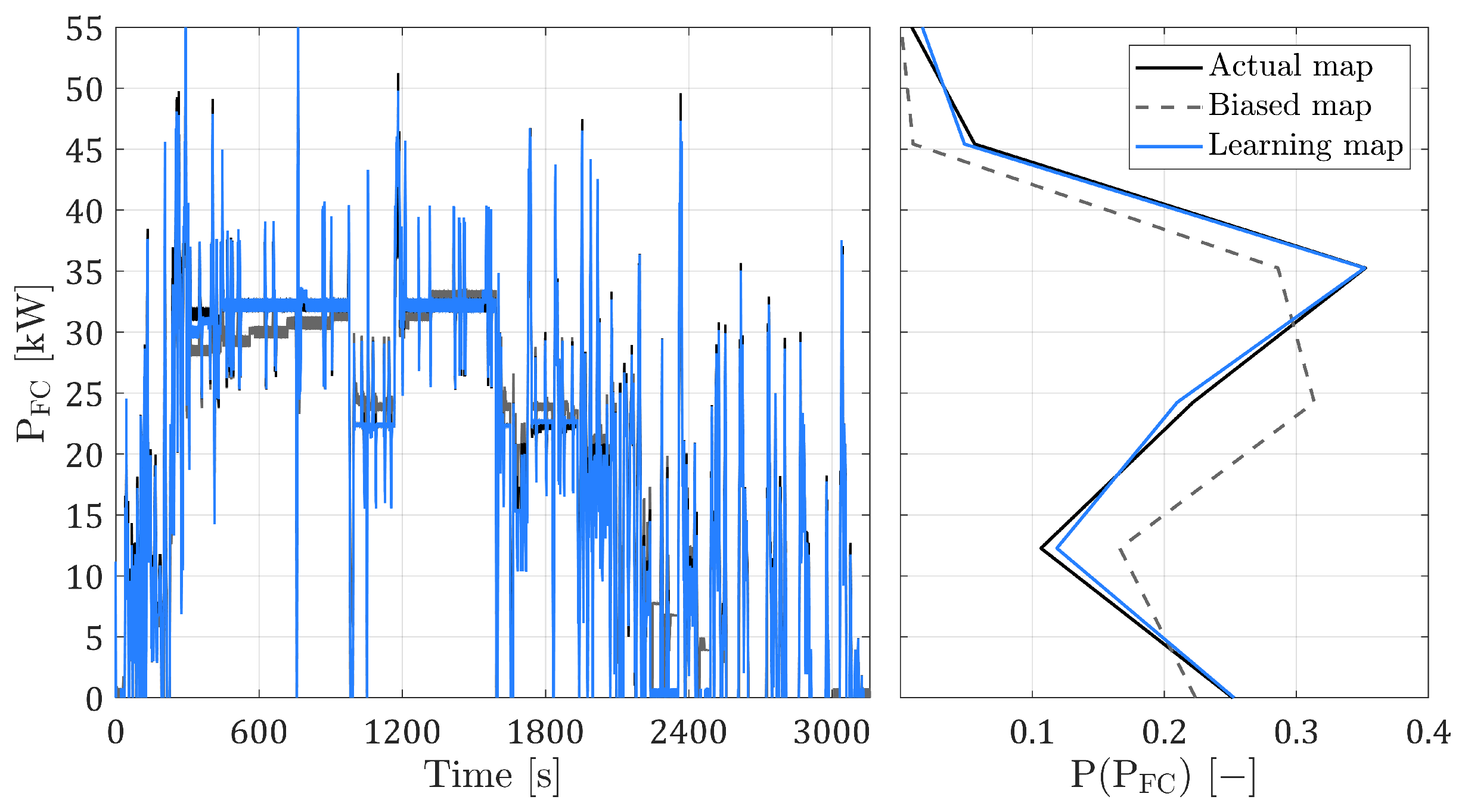
Figure 11 illustrates the impact of the three different maps on EMS control actions for the fuel cell. The left chart shows the evolution of fuel cell output power during the last cycle. In contrast, the right chart depicts the histogram of operation conditions at various fuel cell output power levels. When using the BM, the EMS predominantly controls the fuel cell to operate at medium to low power levels. In contrast, both the AM and the LM guide the EMS to distribute fuel cell operation at mid-range power levels. The high frequency of fuel cell operation at low power with the BM can be attributed to the map’s lower accuracy, as seen in Figure 8. Consequently, the EMS assesses that the BM can provide more power at low and medium current densities for the same current density and hydrogen consumption compared to the other two maps. The importance of fuel model accuracy is highlighted when comparing the histograms of the control action decisions provided by the EMS for each calibration. As the FC model accuracy increases, the EMS can improve the control actions, leading to an expected reduction in fuel consumption.

An important parameter implemented in the algorithm is R (Equation (15b)). This parameter can regulate the Kalman gain of the adapter algorithm. In this case, the higher this value, the lower the gain. Employing a higher R, it is expected that the algorithm slowly adapts the map, thus attributing higher reliability to the map previously implemented in the EMS. On the contrary, for a lower R, the higher the Kalman gain, so the EMS relies more on measuring the fuel cell output power. For this reason, it provides fast adaptation of the map.

Figure 12 presents a parametric study of the proposed method using three different learning rates ($1\times {10}^5$, $7.75\times {10}^4$, and $2.25\times {10}^4$), ranging from slow to fast learning rates, respectively. It is noticed that the proposed method can reduce the error in estimating the fuel cell power, presenting reductions close to 86% in some cycles. For all the learning rates, the proposed method generates strong adaptations to the map in the first 4 h of operation. Then, after this period, the medium and fast learning rates present better accuracy in the map adaptations. In addition, results with faster learning rates prove to be limited, as the algorithm is no longer able to reduce the error, but rather, it generates higher errors due to the dynamic operating conditions of the fuel cell, especially at higher loads. These limitations can be assigned to conditions wherein a sequence of measurements quickly adapt the map, but regardless, the algorithm is not capable of perfectly tracking all the deviations of the model due to the nonlinearity and complexity of the fuel cell system.

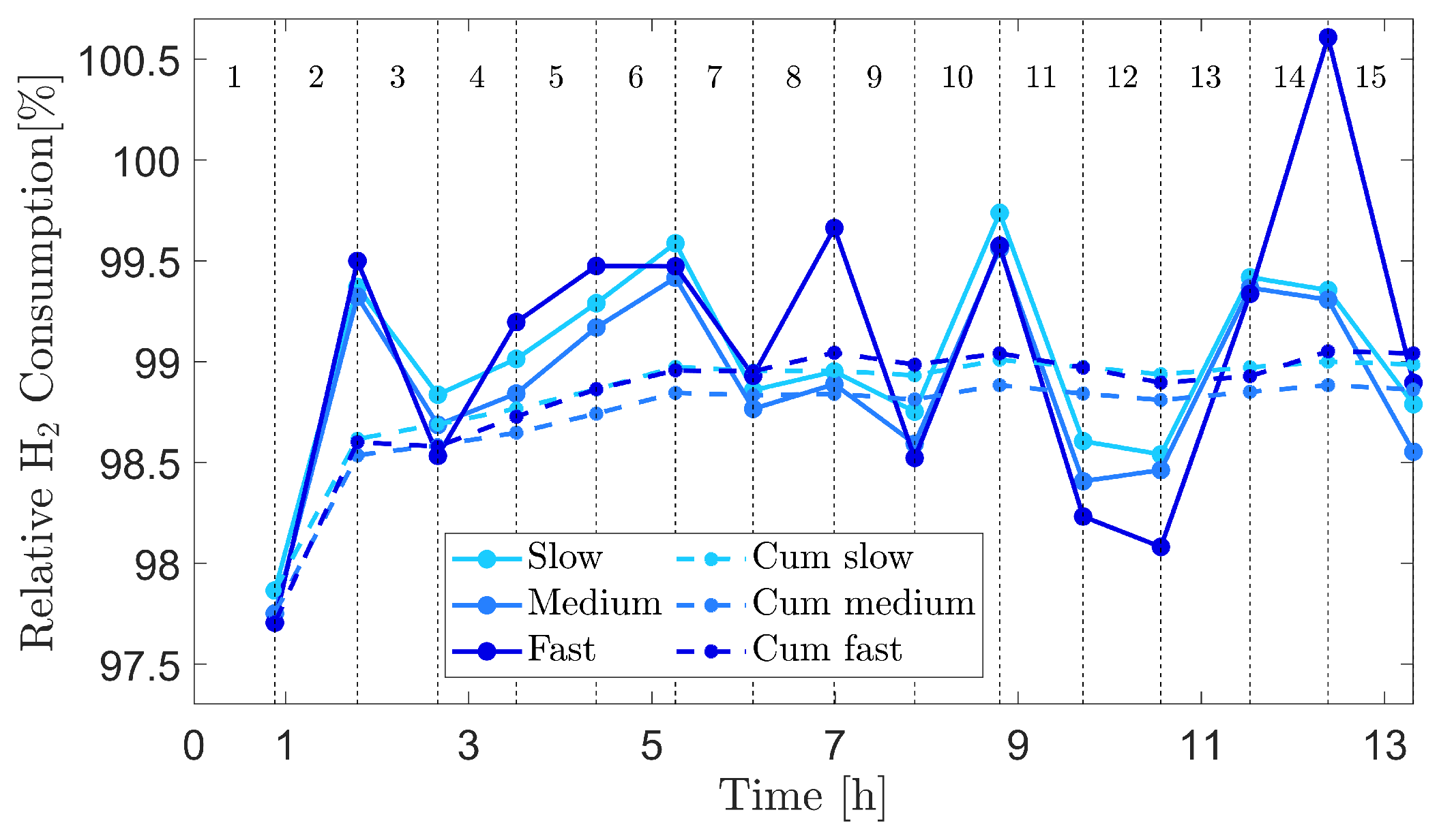
The learning rate also impacted hydrogen consumption, Figure 13 shows the hydrogen consumption for each cycle and also the cumulative hydrogen consumption of all 15 cycles for the slow to fast learning rates. A similar pattern to the reduction in the estimation error in Figure 12 is observed. Furthermore, analysing the consumption cycle to cycle, it is observed that in some cycles, the fast learning rate can overcome the fuel consumption reduction of the medium and slow learning rates, e.g., cycle 3. However, it can also increase hydrogen consumption in some conditions, as observed in cycle 14. However, when comparing the cumulative consumption, the medium learning rate shows slight improvements compared to the other two.

Finally, regarding the map adaptations with the three learning rates, it is demonstrated that the proposed method can guarantee improvements in map calibration up to a certain limit, constrained by the dynamic behaviour of the fuel cell. Furthermore, when comparing the overall performance of different learning rates using the BM as the reference, it becomes evident that in the case of the medium learning rate, the proposed method achieves slight improvements in estimation error and fuel savings considering the set of driving cycles compared to the cases of fast and slow learning rates.

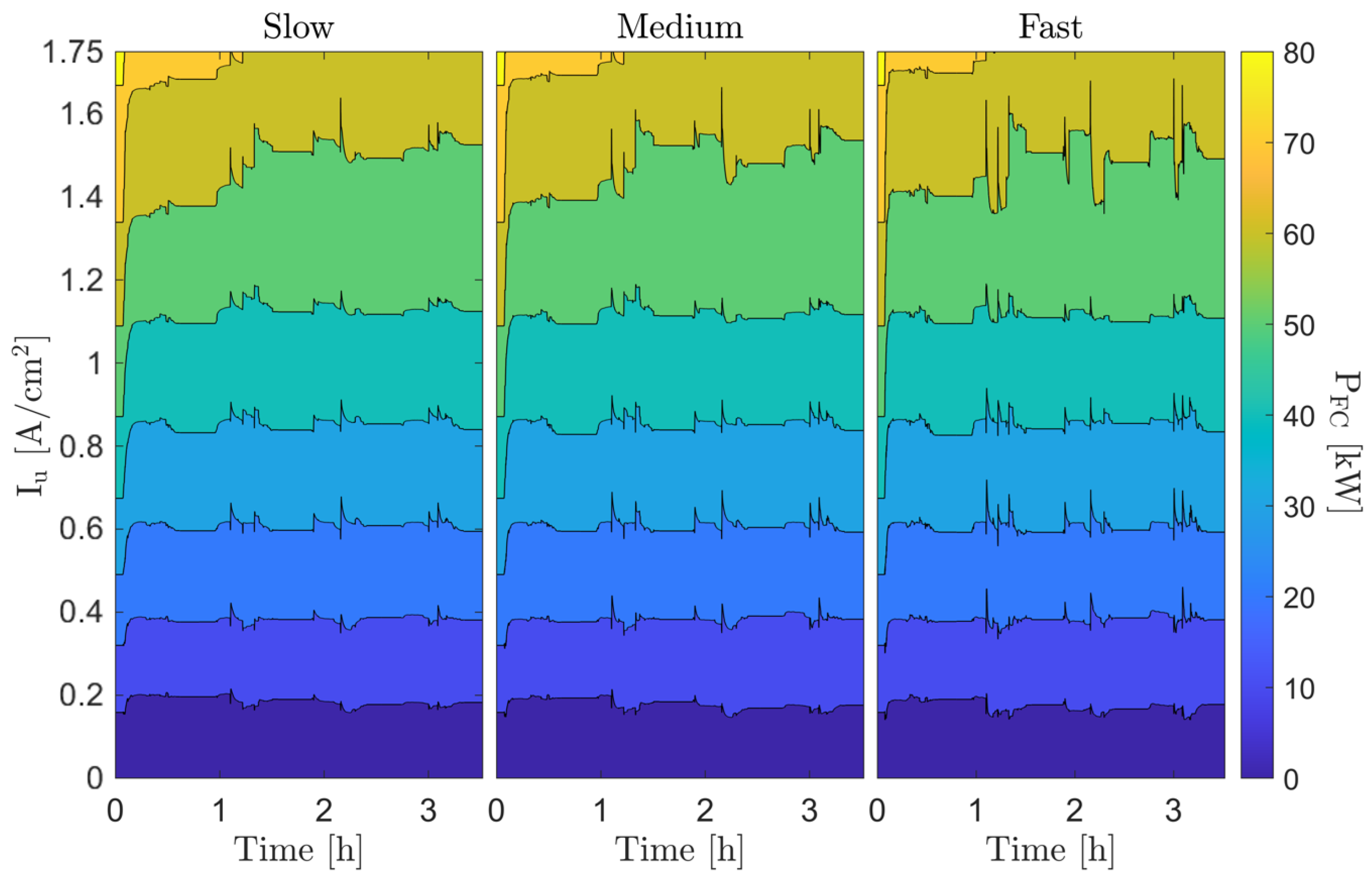
The evolution of map adaptations with three different learning rates is depicted in Figure 14, spanning from the initial operation to the fourth cycle. For all the LM cases, the initial calibration employed is the BM, followed by an ongoing map adaptation as the FCEV operates. All three cases demonstrate the ability to rapidly update the map to match the current output power provided by the FC in the first minutes of operation. In the cases of medium and fast learning rates, the algorithm can adapt the maps quickly, applying stronger corrections to the map for any changes in fuel cell conditions. Conversely, the algorithm applies smoother corrections when employing the low learning rate. In this case, the algorithm requires more time during the initial stages of operation to adapt the map compared to the medium and fast learning rates. Note that in conditions for which the calibration is not being adjusted, the FC is running under the stack warm-up temperature threshold, which is considered to be 340 K.

The proposed method also faces limitations and challenges that warrant attention in future research. Firstly, the stack temperature emerges as a critical parameter influencing FC behaviour, particularly in low-temperature conditions, where the adaptive method ceases operation below the threshold of 340 K. Moreover, higher learning rates exhibit constraints in mitigating FC model errors as they introduce bias to the map adaptations, which limits the capture of FC dynamics in an FC simple map 1D look-up table. Additionally, the reliability and accuracy of FC power measurements are pivotal to the method’s efficacy. Therefore, the selection and assessment of sensors employed to measure FC output power must be thoroughly considered in order to evaluate the feasibility and effectiveness of the method. Addressing these limitations will be crucial for advancing the applicability and robustness of the proposed approach in real-world scenarios.

4. Conclusions

This paper addressed a problem wherein an EMS of an FCEV employs a 1D look-up table to model a fuel cell and compute the power-split using the widespread ECMS. The goal was to adapt the calibration of this model using fuel cell measurements by applying a strategy based on an extended Kalman filter approach. A high-fidelity vehicle plant was modelled to represent the vehicle, and experimental data were employed to build the FC model. Two studies were carried out. The first evaluated EMS performance using three different FC maps. The first map was obtained from a set of steady-state tests on the actual FC. Second, a biased map reproduced the negative impact of modelling errors in model-based control approaches such as the ECMS. Last, we tested the map obtained using the proposed method. The second aspect of the study discussed the learning rate: a parameter that regulates the gain of the adapter algorithm to make higher or lower adaptations to the fuel cell measurements. From the results, we can state that:

• Although a dynamic system such as a fuel cell has been simplified to a 1D look-up table, the proposed method seems to be an option to adapt maps in a model-control-based approach. The proposed method allows us to adjust the look-up table parameters for correcting drift and for slowly varying them when using the vehicle in different driving conditions.
• The primary contribution of this work lies in the adaptive method capability to gradually adjust the map to compensate for any drift resulting from prolonged use. Furthermore, in the case that the EMS utilizes a biased map, significant improvements are shown in short periods of operation: approximately 1 h across various operating conditions.
• The learning algorithm was shown to be advantageous since it improved the estimation of the fuel cell power after only one hour of operation. In addition, it reduced the estimated fuel cell power error by close to 85% compared to the results employing the biased map, providing fuel savings of up to 1.2%.
• The learning rate analysis showed that by using lower learning rates, the algorithm gradually adjusted the map, placing greater trust in the previously implemented map in the EMS. Conversely, when using higher learning rates, the adapter algorithm relied more on the fuel cell power measurement, enabling faster map adaptation.

Regarding future work, the authors may consider the following possible lines:

• Enhance the vehicle model to consider other relevant parameters in the EMS, such as fuel cell air and temperature management as well as battery temperature;
• Increase the map dimensions to incorporate this new parameter in the calibration process, improving the control of the fuel cell system and subsequently improving fuel consumption.

References

1. European Commission. Stepping up Europe’s 2030 climate ambition Investing in a climate-neutral future for the benefit of our people. J. Chem. Inf. Model. 2020, 53, 1689–1699. [Google Scholar]
2. Granovskii, M.; Dincer, I.; Rosen, M.A. Greenhouse gas emissions reduction by use of wind and solar energies for hydrogen and electricity production: Economic factors. Int. J. Hydrogen Energy 2007, 32, 927–931. [Google Scholar] [CrossRef]
3. Salvi, B.L.; Subramanian, K.A.; Panwar, N.L. Alternative fuels for transportation vehicles: A technical review. Renew. Sustain. Energy Rev. 2013, 25, 404–419. [Google Scholar] [CrossRef]
4. Sabri, M.; Danapalasingam, K.; Rahmat, M. A review on hybrid electric vehicles architecture and energy management strategies. Renew. Sustain. Energy Rev. 2016, 53, 1433–1442. [Google Scholar] [CrossRef]
5. Zhuang, W.; Li, S.; Zhang, X.; Kum, D.; Song, Z.; Yin, G.; Ju, F. A survey of powertrain configuration studies on hybrid electric vehicles. Appl. Energy 2020, 262, 114553. [Google Scholar] [CrossRef]
6. Lü, X.; Qu, Y.; Wang, Y.; Qin, C.; Liu, G. A comprehensive review on hybrid power system for PEMFC-HEV: Issues and strategies. Energy Convers. Manag. 2018, 171, 1273–1291. [Google Scholar] [CrossRef]
7. Momirlan, M.; Veziroglu, T.N. The properties of hydrogen as fuel tomorrow in sustainable energy system for a cleaner planet. Int. J. Hydrogen Energy 2005, 30, 795–802. [Google Scholar] [CrossRef]
8. Tanç, B.; Arat, H.T.; Baltacıoğlu, E.; Aydın, K. Overview of the next quarter century vision of hydrogen fuel cell electric vehicles. Int. J. Hydrogen Energy 2019, 44, 10120–10128. [Google Scholar] [CrossRef]
9. Sinigaglia, T.; Lewiski, F.; Santos Martins, M.E.; Mairesse Siluk, J.C. Production, storage, fuel stations of hydrogen and its utilization in automotive applications-a review. Int. J. Hydrogen Energy 2017, 42, 24597–24611. [Google Scholar] [CrossRef]
10. Hosseini, S.E.; Wahid, M.A. Hydrogen production from renewable and sustainable energy resources: Promising green energy carrier for clean development. Renew. Sustain. Energy Rev. 2016, 57, 850–866. [Google Scholar] [CrossRef]
11. Giordano, G. Electric vehicles. Manuf. Eng. 2018, 161, 50–58. [Google Scholar]
12. Onori, S. Hybrid Electric Vehicles Energy Management Strategies; Springer Briefs in Electrical and Computer; Springer: London, UK, 2016. [Google Scholar]
13. Knowles, M.; Ren, Q.; Baglee, D. The state of the art in Fuel Cell condition monitoring and maintenance. World Electr. Veh. J. 2010, 4, 487–494. [Google Scholar] [CrossRef]
14. Alyakhni, A.; Boulon, L.; Vinassa, J.M.; Briat, O. A Comprehensive Review on Energy Management Strategies for Electric Vehicles Considering Degradation Using Aging Models. IEEE Access 2021, 9, 143922–143940. [Google Scholar] [CrossRef]
15. Bayindir, K.Ç.; Gözüküçük, M.A.; Teke, A. A comprehensive overview of hybrid electric vehicle: Powertrain configurations, powertrain control techniques and electronic control units. Energy Convers. Manag. 2011, 52, 1305–1313. [Google Scholar] [CrossRef]
16. Guardiola, C.; Pla, B.; Blanco-Rodriguez, D.; Eriksson, L. A computationally efficient Kalman filter based estimator for updating look-up tables applied to NOx estimation in diesel engines. Control Eng. Pract. 2013, 21, 1455–1468. [Google Scholar] [CrossRef]
17. Kandidayeni, M.; Chaoui, H.; Boulon, L.; Trovao, J.P.F. Adaptive Parameter Identification of a Fuel Cell System for Health-Conscious Energy Management Applications. IEEE Trans. Intell. Transp. Syst. 2021, 23, 7963–7973. [Google Scholar] [CrossRef]
18. Böhler, L.; Ritzberger, D.; Hametner, C.; Jakubek, S. Constrained extended Kalman filter design and application for on-line state estimation of high-order polymer electrolyte membrane fuel cell systems. Int. J. Hydrogen Energy 2021, 46, 18604–18614. [Google Scholar] [CrossRef]
19. Bressel, M.; Hilairet, M.; Hissel, D.; Ould Bouamama, B. Extended Kalman Filter for prognostic of Proton Exchange Membrane Fuel Cell. Appl. Energy 2016, 164, 220–227. [Google Scholar] [CrossRef]
20. Plett, G.L. Extended Kalman filtering for battery management systems of LiPB-based HEV battery packs—Part 3. State and parameter estimation. J. Power Sources 2004, 134, 277–292. [Google Scholar] [CrossRef]
21. Baba, A.; Adachi, S. SOC estimation of HEV/EV battery using series kalman filter. Electr. Eng. Jpn. 2014, 187, 53–62. [Google Scholar] [CrossRef]
22. Guardiola, C.; Pla, B.; Blanco-Rodriguez, D.; Cabrera, P. A learning algorithm concept for updating look-up tables for automotive applications. Math. Comput. Model. 2013, 57, 1979–1989. [Google Scholar] [CrossRef]
23. Höckerdal, E.; Frisk, E.; Eriksson, L. EKF-based adaptation of look-up tables with an air mass-flow sensor application. Control Eng. Pract. 2011, 19, 442–453. [Google Scholar] [CrossRef]
24. Fridholm, B.; Wik, T.; Nilsson, M. Kalman filter for adaptive learning of look-up tables with application to automotive battery resistance estimation. Control Eng. Pract. 2016, 48, 78–86. [Google Scholar] [CrossRef]
25. Yuan, H.; Dai, H.; Wei, X.; Ming, P. A novel model-based internal state observer of a fuel cell system for electric vehicles using improved Kalman filter approach. Appl. Energy 2020, 268, 115009. [Google Scholar] [CrossRef]
26. Xing, Y.; Bernadet, L.; Torrell, M.; Tarancón, A.; Costa-Castelló, R.; Na, J. Offline and online parameter estimation of nonlinear systems: Application to a solid oxide fuel cell system. ISA Trans. 2023, 133, 463–474. [Google Scholar]
27. Gamma Technologies—Home of GT-SUITE System Simulation Software—gtisoft.com. Available online: https://www.gtisoft.com/ (accessed on 21 March 2024).
28. Hyundai. Hyundai Nexo—Technical Specifications. 2023. Available online: https://www.hyundai.com/eu/models/nexo/features.html (accessed on 12 April 2023).
29. Li, J.; Luo, L.; Yang, Q.; Ma, R. A new fuel cell degradation model indexed by proton exchange membrane thickness derived from polarization curve. IEEE Trans. Transp. Electrif. 2022, 9, 5061–5073. [Google Scholar] [CrossRef]
30. Paganelli, G. General supervisory control policy for the energy optimization of charge-sustaining hybrid electric vehicles. JSAE Rev. 2001, 22, 511–518. [Google Scholar] [CrossRef]
31. Paganelli, G.; Guezennec, Y.; Rizzoni, G. Optimizing control strategy for hybrid fuel cell vehicle. SAE Tech. Pap. 2002, 398–406. [Google Scholar] [CrossRef]
Figure 1. Powertrain architecture of the FCEV.
Applsci 14 03473 g001
Figure 2. Maps implemented on the EMS to estimate the fuel cell output power according to the current density input to the vehicle model.
Applsci 14 03473 g002
Figure 3. Recorded vehicle speed traces over time utilized to simulate the vehicle covering different driving conditions in the simulation campaign.
Applsci 14 03473 g003
Figure 4. Fuel cell output power map and polarization curve based on experimental data and models—measured under steady-state conditions.
Applsci 14 03473 g004
Figure 5. Representation of the control-oriented model: above, the vehicle model implemented in GT-Power, and below, the EMS implemented in MATLAB.
Applsci 14 03473 g005
Figure 6. Flowchart of the proposed EKF adaptative algorithm particularized for the 1D look-up table of the case study.
Applsci 14 03473 g006
Figure 7. Evolution of the map adaptations by the adaptive method provided during 15 cycles of operation.
Applsci 14 03473 g007
Figure 8. Operating point distribution of the Learning map during the operation of the 15 cycles and the Evaluated maps. Estimations provided by the Actual map, Biased map, and Learning map are shown in black, gray, and blue, respectively.
Applsci 14 03473 g008
Figure 9. Reduction in the absolute error for the estimation of fuel cell power employing the Actual map and the Learning map compared to the Biased map.
Applsci 14 03473 g009
Figure 10. Relative and cumulative H 2 consumption comparing the Actual map to the Learning map.
Applsci 14 03473 g010
Figure 11. Left plot: Evolution of the FC power signal for the 3 maps in the last cycle. Right plot: Histogram of the operating conditions of the fuel cell power in the driving cycle.
Applsci 14 03473 g011
Figure 12. Reduction in the absolute error in the estimation of fuel cell power comparing three learning rates to the Biased map.
Applsci 14 03473 g012
Figure 13. Relative and cumulative H 2 consumption compared with the that of the Biased map for three learning rates.
Applsci 14 03473 g013
Figure 14. Evolution of the map adaptations by the adaptive method provided during the first four cycles of operation using the three learning rates.
Applsci 14 03473 g014