Parameter Setting for Strategic Buffers in Demand-Driven Material Resource Planning through Statistical Analysis and Optimisation of Buffer Levels

Abstract

The Demand-Driven Material Resource Planning (DDMRP) method is one of the newer methods of inventory management in an enterprise. Its creation was initiated by a change in the business environment and the characteristics of today’s supply chains. DDMRP brings a combined pull/push approach to inventory management based on creating strategic stacks in the supply chain and managing inventory at these strategic points based on customer orders. The DDMRP system provides a simple methodology that is easy to apply, even in smaller businesses, without the need for advanced information systems. However, a simple methodology also has its limitations because, in many cases, intuitive and subjective approaches are used to set inventory management parameters (variability factor, running time factor, seasonality factor, thresholds, etc.). Simplified parameter determination may, under certain conditions, lead to some storage tanks being too high or too low for certain periods of time. We know from classical inventory management, in the conditions of setting stack parameters in DDMRP, that the deficiency can be eliminated by the use of statistical–analytical approaches and optimisation techniques. This article deals with the issue of setting optimal values of storage tanks in DDMRP, while the correctness of the methodology is verified through simulation of the demand-driven planning process. The correctness and usability of the proposed approaches in sizing strategic reservoirs in DDMRP was confirmed through the results of stimulation experiments.

1. Introduction

Conditions under the current inventory management systems are becoming increasingly difficult. Current supply chains tend to be complex in nature, fragmented, and global. The lifecycle of products is short, and the complexity of products is high. This complexity is further enhanced by a high customisation rate and the many configurations and customisations available to individual customers.

Large and fragmented supply chains lead not only to more items being purchased but also to more items being purchased from remote locations, leading to longer delivery times. The combined complexity of the products makes the effort to improve forecast accuracy a losing battle [1].

On the other hand, the rapid development of information technology and the complex integration and implementation of smart solutions using technologies such as IoT, IoS, cloud computing, etc., bring new opportunities in the field of effective enterprise inventory management.

Under these conditions, new concepts and strategies for effective inventory management emerge. One such concept is Demand-Driven Material Requirements Planning (DDMRP). The concept of DDMRP was first systematically described in 2011 in the work of authors Ptak and Smith [1].

DDMRP represents a demand-oriented system of inventory planning and management in an enterprise. It was established as a successor to the MRP system to meet the current requirements of dynamic and turbulent markets. While an MRP system is a pressure inventory management system, a DDMRP system represents a combination of pressure and tensile control principles.

The DDMRP system seeks to eliminate the main shortcoming of the original MRP system, which results from the basic philosophy of dependence of all items in the structure. In the case of item dependencies, any variability (variations in demand, running times, quality deficiencies, system failures, etc.) spreads throughout the logistics–production chain and causes the so-called “bullwhip” effect.

DDMRP tries to stop the transfer of supply chain variability using a basic supply chain “disconnect” mechanism. Disconnection separates one entity from another. This isolates events that occur in one entity or part of a system and prevents them from affecting other entities or parts of the system.

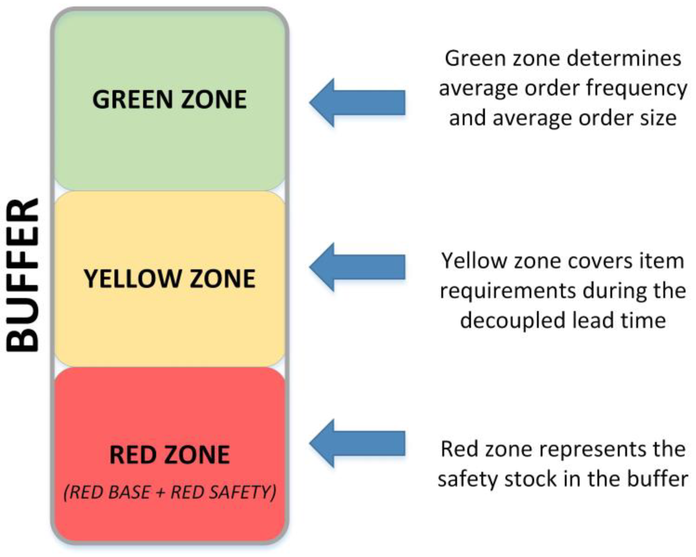
The places where the system is separated are called “decoupling points”. Sufficient inventories must be maintained at the point of disconnection for disconnection points to function as supply chain unbundling and to ensure a sufficient level of protection that absorbs demand and supply variability.

Therefore, one of the key activities of DDMRP is the design of storage tanks at decoupling point buffers and their correct size, which ensures the disconnection of supply and consumption processes and their independence.

The DDMRP system consists of five basic elements that are related to fulfilling the key attributes of the system: position, protect, and pull.

The first three components (strategic inventory positioning, buffer profiles and levels, dynamic adjustments) essentially define the initial configuration of the DDMRP model. The strategic location of inventories will determine where the disconnection points will be located. Tray profiles and levels will determine the level of protection at these disconnection points. Dynamic adjustments define how this level of protection changes upwards or downwards based on operational parameters, changes in the market, and planned or known future events. The fourth (demand-driven planning) and fifth (visible and collaborative execution) elements define the actual operational aspects of a DDMRP system: planning (creating delivery orders) and execution (managing open orders).

Several dozen scientific and professional papers have been published on the issue of DDMRP. A systematic review of scientific papers published up to 2020 devoted to DDMRP issues has been elaborated, for example, in publications by Azzamouri et al. [2] and Orue [3]. Many published papers are devoted to the standardisation and implementation of the DDMRP system in practice [4,5,6,7,8,9,10]. Publications comparing the DDMRP system with other alternative inventory planning and management systems are the second largest group of scientific articles. The DDMRP system, as a combined pressure/tensile system, is compared in individual works with pressure systems, such as MRP and MRP II [11,12,13,14], with the Kanban tensile system [15,16], as well as with alternative combination systems, such as CONWIP [17] and OPT [18].

Further work is devoted to individual elements of the DDMRP system. The authors Abdelhalim et al. [19] and Achergui et al. [20,21] addressed the issue of determining disconnection points and optimally positioning strategic inventories in the supply chain. Achergui et al. [21,22] suggested using the MILP (Mixed-Integer Linear Programming) model to optimise strategic stack positions. The authors paid great attention to determining the parameters of the DDMRP system, whether from the point of view of the primary setting of buffers at disconnection points or from the point of view of their dynamic adjustments in the use phase. In their publication [23], Lee and Rim paid attention to optimising the level of safety stocks in the strategic storage systems of the DDMRP system. Dessevre et al. [24] described dynamic adjustments to the parameter “decoupled lead time” that resulted in the dynamic adjustment of inventory levels in strategic stacks. The dynamic dimensioning of strategic reservoirs is also described in the work of Favaretto et al. [25,26], who used heuristic approaches based on type control (s(t); S(t)) with time-varying thresholds. Duhem et al. [27] discussed the dynamic determination of control parameters OST (order spike threshold) and OSH (order spike horizon). Lahrichi et al. [28] suggested the use of the MILP model in determining strategic reservoir parameters. In their publications [29,30], authors Damand et al. presented a procedure for applying genetic algorithms to determine DDMRP system parameters. In their publication, Martin et al. [31] compared several approaches to sizing DDMRP system parameters from different authors and verified the results using dynamic simulation.

The next part of the publications was devoted to the actual planning and management of inventory in the DDMRP system. In their case study, Iki and Ishak [32] demonstrated the use of a prognostic model of simple exponential smoothing in inventory management in a DDMRP system applied in veterinary medicine. Cuartas and Aguilar [33] described a replenishment algorithm using a learning algorithm based on Markov’s decision-making process. The authors Dessevre et al. [34], Xu et al. [35], and Corsini et al. [36] added part of capacity planning to the planning process in the DDMRP system. Just as unlimited capacities were considered in the MRP system, in the original DDMRP methodology [1], the authors did not consider capacity constraints. However, the capacity planning module represents an important part of inventory planning, especially if the stock in the strategic reservoir is replenished from its own production. Fernandes et al. [37] compared inventory management and order prioritisation based on inventory levels in a strategic stack with classical priority rules (FIFO, Due Date, and ROP) used in manufacturing order management and prioritisation.

As already noted in the literature review, a large group of authors paid attention to setting the parameters of the DDMRP system in their publications. The correct determination of the positions of strategic reservoirs and the dimensioning of their sizes are key prerequisites for the proper functioning of the system in inventory planning and management. It should be noted, however, that most of the authors deviated significantly from the original philosophy of the DDMRP system, as presented by Ptak and Smith [1]. It is characterised by the simplicity of the original methodology, which does not require the implementation of complex specialised systems or advanced mathematical methods and is, therefore, easily applicable in conditions of industrial practice. On the other hand, it must be stated that the original methodology is, in some cases, too benevolent in setting parameters. Simple (naive) determination of insurance stocks can produce worse results than when applying statistical–analytical approaches. The use of naive forecasts in the calculation of ADU (average daily usage) or the use of a demand factor for seasonal items can lead to an inadequate response to system dynamics. Many DDMRP parameters are determined intuitively and subjectively (variability factor, intermediate time factor, seasonality factor, threshold values, etc.). These simplifications may, under more complex conditions, result in some storage facilities being oversized or undersized over periods of time, and thus not being able to perform their basic functions efficiently. The aim of this article is to fill the gap between the original simple methodology of setting parameters for strategic reservoirs and the complex approaches of individual authors, which are presented in scientific articles devoted to this issue. The approach of the authors, which will be presented in the next sections, preserves the simplicity of the original methodology but at the same time introduces, into the process of setting the parameters of the reservoir, a simple mathematical apparatus based on statistical–analytical and optimisation procedures known from classical inventory management in the company, thus eliminating decision-making based on intuition, estimation, or expert assessment from the process of sizing reservoirs. At the same time, the proposed storage sizing approach will be compared with the original sizing approach described in [1]. To evaluate and compare the results of both approaches, a simulation of the planning process (generation of delivery orders) will be used.

2. Materials and Methods

2.1. Buffer Zones and Their Dimensioning According to Ptak and Smith

Strategic reservoirs in DDMRP serve three basic purposes [1]:

• Shock absorption: Dampening both supply and demand variability greatly reduces or eliminates the transmission of variability, which creates jitteriness and a bullwhip effect in the chain.
• Reduced running time: Separating the continuous time of the supplier from the consumable side of the tank immediately reduces lead times.
• Delivery order generation: All relevant demand information, delivery information, and inventory information are combined in the warehouse to create a “net flow equation” that is used in the planning and calculation of delivery orders. Thus, stacks are the heart of the scheduling system in DDMRP.

The standard tray in DDMRP consists of three zones [38] (Figure 1):

• Green zone: The green zone is the heart of the order generation process. It specifies the average frequency of orders and the typical order size.
• Yellow zone: The yellow zone covers the average need for an item during the rolling delivery time. The yellow zone is always calculated as the product of average daily usage and decoupled lead time.
• Red zone: The red zone is a security component embedded in the tray. It consists of two parts (a red base, and a red safety). The higher the variability associated with an item, the larger the red zone will be.

The size of individual zones according to the Ptak and Smith methodology is determined depending on the combination of the stack profile and the individual characteristics of the item [7].

Container profiles enable practical and efficient global management of large quantities of strategically disconnected parts. They represent a grouping of parts or similar characteristics. Tray profiles are families or groups of parts for which it makes sense to design a set of rules, guidelines, and procedures that can be applied in the same way to all members of that profile. For tray profiles, according to [1], the similarity of items is formed on the basis of three specific factors:

• Item type (P—purchased items, M—manufactured items, D—distributed items).
• Lead time (S—short, M—medium, L—long). For manufactured parts, decoupled lead time (DLT) should be taken into account when evaluating the length of the running time.
• Variability (H—high, M—medium, L—low). When determining the profile of a storage tank, two types of variability are determined: demand variability (which assesses the risk of sharp fluctuations in the need for a given item) and supply variability (which assesses the risk and severity of failures in the sources of supply of a given item).

According to the assigned stack profile, the stack is assigned a lead time factor and a variability factor. The values of the factors are determined on the basis of expert judgement from a range of recommended values (1).

2.1.1. Green Zone Calculation

The green zone can be determined based on one of three factors. The factor that yields the greatest value determines the resulting size of the green zone [7]:

(a)

Calculation based on DOC (desired order cycle)

GZ1 = ADU × DOC,

(1)

where:

• GZ1—green zone based on desired order cycle,
• ADU—average daily usage,
• DOC—desired order cycle.

(b)

Calculation based on LTF (lead time factor)

GZ2 = DLT × ADU × LTF,

(2)

where:

• GZ2—green zone based on lead time factor,
• DLT—decoupled lead time,
• ADU—average daily usage,
• LTF—lead time factor.

(c)

Calculation based on MOQ (minimum order quantity)

GZ3 = MOQ,

(3)

where:

• GZ23—green zone based on minimum order quantity,
• MOQ—minimum order quantity.

The resulting green zone value is determined as:

GZ = max (GZ1, GZ2, GZ3).

(4)

2.1.2. Yellow Zone Calculation

The yellow zone covers the average consumption of the item during its delivery time. The yellow zone is always calculated as [7]:

YZ = ADU × DLT,

(5)

2.1.3. Red Zone Calculation

The red zone provides a safety function in the tray. The higher the variability associated with a given item, the larger the red zone will be. The calculation of the red zone is carried out in the following three steps [7]:

1.

Red base calculation:

Red base represents basic safety stock in the buffer. It takes into account the change in the risk of deviations depending on the length of the decoupled lead time. It is calculated as:

RB = ADU × DLT × LTF,

(6)

2.

Red safety calculation:

Red safety takes into account the variability rate of the basic parameters at the buffer input and output: demand spikes and supply interruptions. It is calculated as:

RS = RB × VF,

(7)

where:

• VF—variability factor.

3.

Red zone calculation:

RZ = RB + RS.

(8)

2.2. Methodology of Buffer Zones’ Dimensioning

The proprietary methodology of sizing strategic reservoirs, proposed by the authors, consists of four basic steps (Figure 2):

• Input data preparation,
• Statistical analysis of input data,
• Calculation of optimal inventory control parameters,
• Buffer zone setting.

A prerequisite for applying the methodology is knowledge of strategic inventory positions (disconnection points) in the DDMRP system. The proprietary methodology then solves the problem of sizing the storage tank at a specific point of disconnection. The following section explains the content of the single steps of the methodology.

2.2.1. Input Data Preparation

The main baseline data for statistical analysis and subsequent dimensioning of the reservoir are [39]:

• parameters of the delivery process: lead time, order quantity, or order cycle (and their variability),
• parameters of consumption: average daily usage, usage variability.

The parameters of the delivery process are defined on the basis of the delivery conditions of the material in the case of replenishment of stocks from external sources (suppliers) or on the basis of the parameters of the production of the part in the case of replenishment of stocks from own sources (from own production). To set the tray parameters, it is not enough to consider only the declared (or average) parameter values. To assess the variability of individual parameters, it is necessary to compile a series of historical data:

• series of daily usages,
• series of lead time values,
• series of delivery quantities vs. series of order quantities.

The minimum length of the data series should cover a time horizon of at least one year, so that the analysis evaluates the possible effects of seasonality. These data were obtained from the consumption records and delivery process in the company’s information system.

2.2.2. Statistical Analysis of Input Data

The prepared series of data were subjected to statistical analysis. The output of statistical consumption analysis was the determination of the basic parameters of a random variable (Figure 3)—daily consumption (average consumption, standard deviation, and type of distribution). The calculated average value represents the ADU (average daily usage) value in DDMRP. The variability of daily consumption was processed in the form of a cumulative probability distribution function (Figure 4). This cumulative function was used when sizing the first tranche of the buffer stock.

In a similar way as in the case of daily consumption, the statistical analysis of the lead time was also carried out. The basic parameters of the random variable (average lead time, standard deviation, and distribution type) were determined. The calculated average value represents the decoupled lead time (DLT) value in DDMRP. The variability of the lead time was processed in the form of a cumulative probability distribution function. This cumulative function was used when sizing the second portion of the buffer stock [40].

The third part of the statistical analysis was the analysis of historical data on a series of delivery sizes. Statistical analysis consisted of comparing paired values: ordered quantity vs. delivered quantity (Figure 5). A new time series was created from the values:

QV = DQ − OQ,

(9)

where:

• QV—quantity variation,
• DQ—delivered quantity,
• OQ—ordered quantity.

This analysis resulted in a cumulative probability distribution function for quantity variations (Figure 6).

2.2.3. Calculation of Optimal Inventory Control Parameters

When calculating optimal inventory management parameters, we based our calculations on well-known order policies. These policies apply tensile inventory management principles. The DDMRP system represents a pressure–tensile steering system. Stocks in strategic DDMRP storage systems are replenished based on tensile signals, and stocks within one loop between two downstream disconnection points are controlled by pressure principles.

• P systems (fixed-order period systems): These are replenishment systems operating with a fixed order cycle. Orders for new deliveries are executed at regular time intervals, and the size of the order is usually variable. The determination of the basic parameters of the P system involves the calculation of the order cycle length, premium, and maximum (after-order) inventory level. The advantage of P systems is the lower difficulty of monitoring the development of inventory levels (inventory levels are evaluated periodically) and the possibility of ordering several items together (in the case of determining a common length of the order cycle). The disadvantage is the lower flexibility of the system for the real development of the inventory of items in stock and the need to hold a higher buffer stock.
• Q systems (fixed-order quantity systems): These systems work with fixed order sizes and variable ordering dates. Ordering a new delivery is realised when the stock drops below the ROL (reorder level). The determination of the basic parameters of the Q system includes the calculation of the buffer stock, the signal inventory level (ROL), and the optimal order size. The advantage of Q systems is their ability to quickly react to changes in inventory levels and lower insurance stocks, while the disadvantage is the higher labour costs of inventory monitoring (continuous monitoring of inventory development).

For the purpose of calculating basic inventory parameters, a combined ordering policy was used, which works with variable ordering dates and variable order sizes. This combination ensures the best inventory level flexibility for different types of variability and corresponds to the strategic storage management philosophy in the DDMRP concept.

The basic parameters of inventories and the method of determining them are as follows:

1.

Safety stock:

The buffer stock consists of three basic components:

• insurance against the variability of consumption,
• insurance against the variability of the lead time,
• insurance against the variability of delivery sizes.

The starting point for determining the optimal level of the buffer stock is the calculation of the optimal service level [41]:

$$\mathrm{S}\mathrm{L}=\frac{{\mathrm{C}}_{\mathrm{s}}}{{\mathrm{C}}_{\mathrm{s}}+{\mathrm{C}}_{\mathrm{c}}}\times 100$$

(10)

where:

• SL—optimal service level (%),
• C_s—stockout cost (EUR/(unit × day)),
• C_c—carrying cost (EUR/(unit × day)).

For a specified level of service, from the cumulative probability distribution functions (variations in consumption, variations in lead time, and variations in quantity), the required degree of coverage was assigned a corresponding insurance component (Figure 7).

The resulting buffer stock was determined as:

SS = Sd + ADU × S_l + Sq,

(11)

where:

• SS—safety stock (units),
• Sd—safety against the variability of demand (units),
• S_l—safety against the variability of lead time (days),
• Sq—safety against the variability of delivered quantity (units),
• ADU—average daily usage.

2.

Reorder level:

The signal level must be set to cover the average consumption of the item during the lead time, and the stock of the item must be replenished exactly at the moment when its level reaches the minimum, i.e., safety stock:

ROL = SS + ADU × DLT,

(12)

3.

Maximum stock level:

The maximum inventory level was set to cover material consumption during one inventory turnover and to replenish the stock in an optimal ordering cycle. The optimal ordering cycle was determined using the formula for the POQ (periodic order quantity) inventory model [42]:

$$\mathrm{O}\mathrm{C}=\sqrt{\frac{2\times {\mathrm{C}}_{\mathrm{o}}}{\mathrm{A}\mathrm{D}\mathrm{U}{\mathrm{C}}_{\mathrm{c}}}}$$

(13)

where:

• OC—order cycle (days),
• C_o—ordering cost (EUR/order),
• C_c—carrying cost (€EUR/(unit × day)),
• ADU—average daily usage.

The maximum stock was then determined as:

MSL = ROL + OC × ADU,

(14)

2.2.4. Buffer Zone Setting

The calculated optimal inventory management parameters were then transformed into buffer zone sizes in accordance with the DDMRP system rules, as follows:

RZ = SS,

(15)

YZ = ROL − SS,

(16)

GZ = OC × ADU,

(17)

TOR = RZ,

(18)

TOY = RZ + YZ = ROL,

(19)

TOG = RZ + YZ + GZ = ROL + OC × ADU,

(20)

where:

• RZ—red zone,
• YZ—yellow zone,
• GZ—green zone,
• TOR—top of red,
• TOY—top of yellow,
• TOG—top of green.

2.3. Verification of Proposed Methodology

Methodology verification was carried out for a strategic stack of a sample item whose basic parameters were known (

Table 1. Basic parameters of the example item.

Average Daily Usage (ADU)	30
Buffer profile:	M, M, M
-lead time factor (LTF)	0.5
-variability factor (VF)	0.5
Minimum order quantity (MOQ)	50
Desired order cycle (DOC)	8
Decoupled lead time (DLT)	5
Ordering cost (EUR/order)	1000
Carrying cost (EUR/(piece × day))	2
Stockout cost (EUR/(piece × day))	38

). It is a manufactured item with a medium lead time length and a medium level of variability (buffer profile = M, M, M). In addition to the data presented in the table, there are a series of historical data that are necessary for evaluating the variability of consumption, lead time, and delivery quantity (see Section 2.2.3). Parameters in the Table 1 have been determined based on the delivery terms of the item (MOQ and DOC), the analysis of historical consumption data (ADU), the inventory cost structure (ordering cost, carrying cost, and stockout cost), and the basic DDMRP system settings (DLT, LTF, and VF).

The sample item was subjected to a series of simulation experiments based on simulating the process of generating delivery orders [43,44,45]. As part of the simulation, the following sets of experiments were carried out:

• Simulation of the process of generating delivery orders with the default setting of the buffer parameters according to Ptak and Smith’s methodology [1] (Table 1).
• Simulation of the impact of a change in the item output parameters on the efficiency parameters of the inventory replenishment process—one-factor analysis:
  • change of lead time factor (simulated LTF values: 0.1, 0.3, 0.5, 0.7, and 0.9),
  • change of variability factory (simulated VF values: 0.1, 0.3, 0.5, 0.7, and 0.9),
  • change of desired order cycle (simulated DOC values: 4, 6, 8, 10, and 12 days).
• Simulation of the impact of a change in the item input parameters (LTF, VF, and DOC) on the parameters of the efficiency of the inventory replenishment process—multifactor analysis.
• Simulation of the process of generating delivery orders with the setting of buffer parameters according to the methodology of the authors, described in Section 2.2.

In the simulation of individual variants, the procedure for generating delivery orders according to the demand-driven planning methodology [1] was used. A simulation model was created that simulates random inputs to the simulation based on the probability distribution of input quantities found in the input statistical analysis:

• random daily usage,
• random variations of lead time,
• random variations in delivered quantity.

The order generation process itself was based on calculating the net flow equation [1]:

NFP = OH + OO − QD

(21)

where:

• NFP—net flow position,
• OH—on hand (the quantity of stock physically available),
• OO—on order (the quantity of stock that has been ordered but not received),
• QD—qualified sales order demand (the sum of sales orders past due, sales orders due today, and qualified spikes).

Within the simulation model, thresholds were set to:

• order spike threshold: OST = 0.5 × RZ,
• order spike horizon: OSH = DLT + 1.

The duration of the simulation run was 1 calendar year (250 working days). Every day, the simulation model calculated a value called net flow position (NFP) using the net flow equation. The net flow position determines whether generating a new delivery order is recommended in the stack. If the position is below the upper limit of the yellow zone (TOY, top of yellow), then a quantity delivery order is generated, which is calculated as the difference between the net flow position and the upper limit of the green zone (TOG, top of green). The structure of the simulation table is shown in Figure 8.

The outputs of the simulation experiments were used to evaluate the efficiency of the order generation process and assess the appropriateness of setting stack parameters. The simulation model provided the following outputs:

• progress of the on-hand inventory and net flow position (Figure 9a),
• histogram of on-hand inventory distribution (Figure 9b),
• summary outputs:

  ○

  service level,

  ○

  average inventory level,

  ○

  orders count,

  ○

  average order cycle,

  ○

  average order quantity,

  ○

  total inventory cost.

3. Results

In this section, simulation results for individual sets of simulation experiments will be presented in turn.

3.1. Default Setting of Buffer Parameters According to Ptak and Smith’s Methodology

The sample item parameters are listed in Table 1. Based on these parameters, buffer zone sizes and basic parameters for generating delivery orders (

Table 2. Default buffer setting.

Green zone (resulting value)	240
GZ1	240
GZ2	75
GZ3	50
Yellow zone (resulting value)	150
Red zone (resulting value)	113
Red base	75
Red safety	38
TOG (top of green)	503
TOY (top of yellow)	263
TOR (top of red)	113
Order spike threshold (OST)	56.5
Order spike horizon (OSH)	6

) were calculated.

Subsequently, a set of simulation experiments was carried out, and the output parameters of the simulation were evaluated (

Table 3. Summary results of simulation experiments (default buffer setting).

	Min.	Average	Max.
Service level (%)	97.13	99.55	100.00
Average inventory (pcs)	213.77	222.42	234.46
Orders per year	31.00	32.40	34.00
Average order cycle (days)	7.35	7.72	8.06
Average order quantity (pcs)	261.97	266.05	270.47
Total inventory cost (EUR)	138,926.00	144,973.60	151,498.00

and Figure 10).

The values of the simulation output parameters from the default buffer setting represent a comparison with the results of other simulation experiments for assessing changes in inventory management efficiency when the buffer parameters were changed.

3.2. Changing the Setting of Buffer Input Parameters—Single-Factor Analysis

The objective of this set of simulation experiments was to assess how a change in the input parameter will affect the values of the simulation output parameters. In each set of simulation experiments, the value of only one input parameter changed, while the values of the other parameters remained the same as in the default buffer settings.

3.2.1. Change in Lead Time Factor

The aim of this experimental part was to evaluate the impact of a change in the lead time factor (LTF) value on the inventory management efficiency and output parameter value. In this set of simulation experiments, LTF = {0.1, 0.3, 0.5, 0.7, 0.9} were sequentially simulated. The simulation results are shown in

Table 4. Summary results of simulation experiments (change in LTF).

Lead Time Factor	Service Level (%)			Average Inventory (pcs)			Total Inventory Cost (EUR)
	Min.	Average	Max.	Min.	Average	Max.	Min.	Average	Max.
0.1	99.48%	99.92%	100.00%	235.86	243.95	248.28	152,488.0	155,821.8	158,138.0
0.3	99.40%	99.84%	100.00%	228.08	238.22	253.34	146,522.0	152,885.0	160,670.0
0.5	97.13%	99.49%	100.00%	213.77	222.89	234.46	138,926.0	145,175.0	151,498.0
0.7	99.69%	99.97%	100.00%	243.36	253.34	260.30	155,682.0	159,762.6	162,152.0
0.9	100.00%	100.00%	100.00%	279.06	287.30	297.84	172,532.0	175,750.2	179,922.0

and Figure 11.

The simulation results showed that the best inventory management parameters were achieved by the strategic sample item buffer when setting the LTF = 0.5 value. Although a slightly lower real service level was achieved at this LTF value (average = 99.49%), this value still far exceeded the baseline requirement (service level = minimum 95%).

3.2.2. Change in Variability Factory

The aim of this experimental part was to evaluate the impact of changing the value of the variability factor (HF) on the efficiency of inventory management and the value of output parameters. In this set of simulation experiments, VF = {0.1, 0.3, 0.5, 0.7, 0.9} were sequentially simulated. The simulation results are shown in

Table 5. Summary results of simulation experiments (change in VF).

Variability Factor	Service Level (%)			Average Inventory (pcs)			Total Inventory Cost (EUR)
	Min.	Average	Max.	Min.	Average	Max.	Min.	Average	Max.
0.1	97.99%	99.29%	100.00%	215.52	224.78	234.28	140,758.0	147,108.2	154,180.0
0.3	98.21%	99.15%	100.00%	209.38	218.83	229.04	142,852.0	145,067.8	147,376.0
0.5	97.13%	99.55%	100.00%	213.77	222.42	234.46	138,926.0	144,973.6	151,498.0
0.7	99.48%	99.91%	100.00%	230.34	239.50	251.63	147,424.0	153,015.8	158,944.0
0.9	99.27%	99.86%	100.00%	227.82	244.66	251.47	147,868.0	155,444.6	159,130.0

and Figure 12.

The simulation results in this case are no longer as clear-cut as in the case of the change in LTF. From the point of view of the average inventory level, the best setting seemed to be the parameter VF = 0.3. However, the average cost of inventory in this case was slightly higher than with the setting VF = 0.5, which may be due to a lower service level (average service level = 99.15%). On the other hand, a value of VF = 0.3 recorded a significantly lower dispersion of values of output parameters (service level and total inventory cost) than VF = 0.5.

3.2.3. Change in Desired Order Cycle

The last part of the one-factor analysis was to evaluate the impact of changing the value of the desired order cycle (DOC) on the efficiency of inventory management and the value of the output parameters. In this set of simulation experiments, DOC = {4, 6, 8, 10. 12 days} values were sequentially simulated. The simulation results are displayed in

Table 6. Summary results of simulation experiments (change in DOC).

Order Cycle	Service Level (%)			Average Inventory (pcs)			Total Inventory Cost (EUR)
	Min.	Average	Max.	Min.	Average	Max.	Min.	Average	Max.
4	99.03%	99.66%	100.00%	167.70	174.08	185.68	142,928.0	146,572.8	150,126.0
6	99.08%	99.80%	100.00%	196.94	203.76	211.02	140,470.0	144,770.8	148,912.0
8	97.13%	99.55%	100.00%	213.77	222.42	234.46	138,926.0	144,973.6	151,498.0
10	99.52%	99.85%	100.00%	239.24	255.88	270.79	147,618.0	155,378.2	162,394.0
12	98.67%	99.62%	100.00%	267.19	282.78	294.10	157,508.0	164,836.8	174,052.0

and Figure 13.

The results of the simulation confirmed the direct dependence of the average stock on the length of the order cycle. The longer the order cycle, the larger the order quantity must be, and the larger the average stock [44]. Therefore, from the point of view of inventory levels, it would be ideal to use a minimum order cycle. However, shortening the ordering cycle led to an increase in order costs. From the point of view of the minimum total cost, the optimal value seemed to be DOC = 6 days. Not only did it ensure the lowest value of total inventory costs (average total inventory cost = EUR 144,770.8), but at the same time, the simulation experiments showed a very low dispersion of output parameter values at this DOC value.

3.3. Changing the Setting of Buffer Input Parameters—Multifactor Analysis

Another part of the simulation experiments was to evaluate the impact of the simultaneous change of several input factors (LTF, VF, and DOC) on the inventory management efficiency of the sample item and the value of the output parameters of the inventory management system. For the design of experiments, the Taguchi method was used, and an orthogonal field P = 3, L = 3, formed by three input factors (LTF, VF, and DOC) and three levels of factors was created. Three factor values were selected as the factor levels that yielded the best results in single-factor analysis (

Table 7. Orthogonal array P = 3, L = 3.

	Factors
Levels	LTF	VF	DOC
1	0.1	0.1	4
2	0.3	0.3	6
3	0.5	0.5	8

).

The Taguchi experiment plan for the orthogonal field P = 3, L = 3 is shown in

Table 8. Taguchi design (factor levels).

Experiment	LTF	VF	DOC
EX1	1	1	1
EX2	1	2	2
EX3	1	3	3
EX4	2	1	2
EX5	2	2	3
EX6	2	3	1
EX7	3	1	3
EX8	3	2	1
EX9	3	3	2

and

Table 9. Taguchi design (factor values).

Experiment	LTF	VF	DOC
EX1	0.1	0.1	4
EX2	0.1	0.3	6
EX3	0.1	0.5	8
EX4	0.3	0.1	6
EX5	0.3	0.3	8
EX6	0.3	0.5	4
EX7	0.5	0.1	8
EX8	0.5	0.3	4
EX9	0.5	0.5	6

.

The results of simulation experiments EX1–EX9 are presented in the summary table (

Table 10. Summary results of the simulation experiments (multifactor analysis).

Experiment	Service Level (%)			Average Inventory (pcs)			Total Inventory Cost (EUR)
	Min.	Average	Max.	Min.	Average	Max.	Min.	Average	Max.
EX1	99.37%	99.77%	100.00%	185.61	191.50	195.90	155,164.0	157,046.0	160,296.0
EX2	98.21%	99.75%	100.00%	201.68	213.16	224.12	146,078.0	150,440.8	154,058.0
EX3	99.48%	99.92%	100.00%	235.86	243.95	248.28	152,488.0	155,821.8	158,138.0
EX4	99.55%	99.92%	100.00%	213.60	224.95	231.91	149,280.0	155,118.0	157,954.0
EX5	99.00%	99.65%	100.00%	236.45	246.11	260.05	150,226.0	156,520.8	164,346.0
EX6	99.53%	99.84%	100.00%	178.69	185.40	193.56	147,746.0	149,768.0	152,966.0
EX7	97.99%	99.29%	100.00%	215.52	224.78	234.28	140,758.0	147,108.2	154,180.0
EX8	99.21%	99.71%	100.00%	165.17	171.67	179.45	143,012.0	145,093.8	147,926.0
EX9	98.51%	99.42%	100.00%	197.83	201.52	209.43	142,076.0	144,009.6	146,684.0

) and the values of the output parameters are visualised in Figure 14 and Figure 15.

The multifactor analysis results showed that the best results in terms of minimising total inventory costs were achieved with the EX9 experiment, which corresponds to the setting of input parameters at the levels: LTF = 0.5, VF = 0.5, and DOC = 6 days.

As described in Section 3.2 and Section 3.3, the simulation experiments enabled us to objectify the setting of the sample item strategic buffer using standard input parameters of the DDMRP methodology (

Table 11. Buffer setting after input factors’ objectification.

Green zone (resulting value)	180
GZ1	180
GZ2	75
GZ3	50
Yellow zone (resulting value)	150
Red zone (resulting value)	113
Red base	75
Red safety	38
TOG (top of green)	443
TOY (top of yellow)	263
TOR (top of red)	113
Order spike threshold (OST)	56.5
Order spike horizon (OSH)	6

).

3.4. Setting of Buffer Input Parameters Using Authors’ Own Methodology

The last set of simulation experiments was applied with the setting of buffer parameters according to the authors’ own methodology, which was described in Section 2.2. Calculations of basic inventory parameters and dimensioning of individual buffer zones for a sample item are summarised in

Table 12. Buffer setting using authors’ own methodology.

Parameter	Value
Optimum service level	=38/(38 + 2) × 100 = 95%
Safety against the variability of demand	=17 pcs
Safety against the variability of lead time	=3 days
Safety against the variability of delivered quantity	=20 pcs
Safety stock	=17 + 3 × 30 + 20 = 127
Reorder level	=127 + 30 × 5 = 277
Order cycle	=SQRT((2 × 1 × 1000)/(2 × 30)) = 6 days
Red zone	=127
Yellow zone	=277 − 127 = 150
Green zone	=6×30 = 180
TOG (top of green)	=127 + 150 + 180 = 457
TOY (top of yellow)	=127 + 150 = 277
TOR (top of red)	=127
Order spike threshold (OST)	=0.5×127 = 63.5
Order spike horizon (OSH)	6

.

The results of the simulation experiments are summarised in

Table 13. Summary results of simulation experiments (buffer setting—authors’ own methodology).

Experiment	Min.	Average	Max.
Service level (%)	99.75%	99.94%	100.00%
Average inventory (pcs)	193.78	202.60	210.31
Orders per year	40.00	41.20	44.00
Average order cycle (days)	5.68	6.07	6.25
Average order quantity (pcs)	202.48	207.98	214.66
Total inventory cost (EUR)	138,932.00	142,690.40	146,156.00

and Figure 16.

4. Discussion

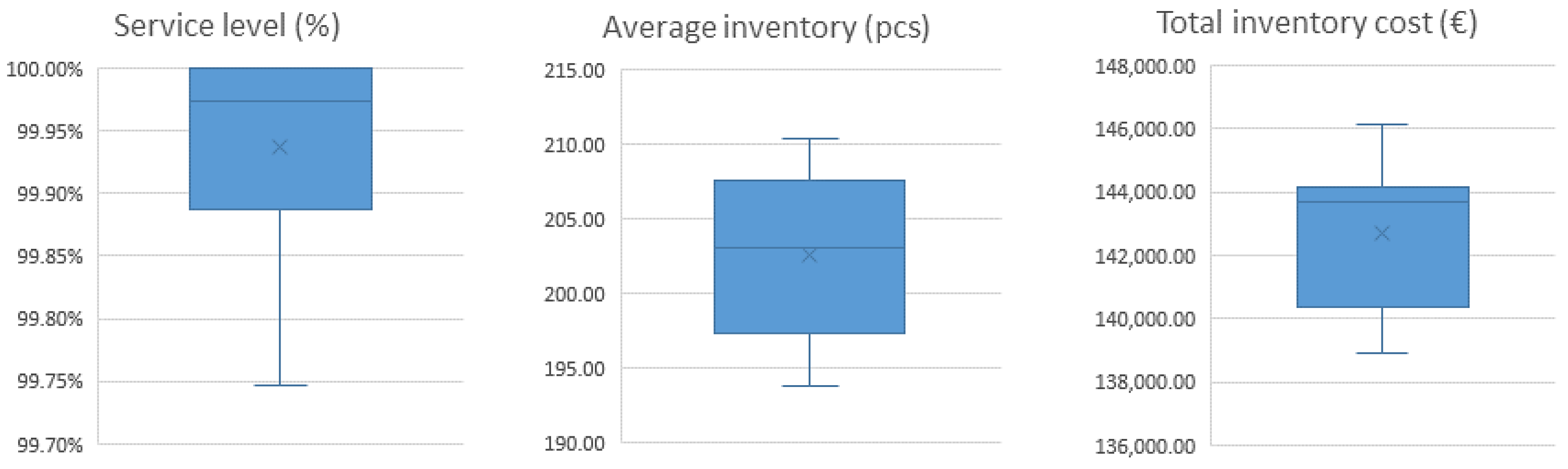
At the end of this article, we compare the values of inventory management output parameters when sizing a stack in three basic ways (

Table 14. Comparison of the results of the simulation experiments.

Experiment	Service Level (%)			Average Inventory (pcs)			Total Inventory Cost (EUR)
	Min.	Average	Max.	Min.	Average	Max.	Min.	Average	Max.
Default buffer setting	97.13	99.55	100.00	213.77	222.42	234.46	138,926.0	144,973.6	151,498.0
Buffer setting objectification	98.51	99.42	100.00	197.83	201.52	209.43	142,076.0	144,009.6	146,684.0
Buffer setting optimisation	99.75	99.94	100.00	193.78	202.60	210.31	138,932.0	142,690.4	146,156.0

and Figure 17):

• Default buffer setting (Section 3.1): This method assumes setting the parameters of the strategic stack using the original calculation methodology according to Ptak and Smith.
• Buffer setting objectification (Section 3.2): This method used a series of simulation experiments to improve the default buffer setting. The objectification of parameters took place in two phases. In the first phase, a one-factor analysis (parameters LTF, VF, and DOC) was carried out. Based on the results of the single-factor analysis and using the Taguchi method, a series of simulation experiments was planned and implemented in the second phase as part of the multifactor analysis.
• Buffer setting optimisation (Section 3.3): The third method used the original methodology of sizing the parameters of the stack, as proposed by the authors of the article. This methodology combines procedures for statistical analysis of historical data (determination of safety stock) and inventory management policies, working with the determination of reorder levels and the maximum stock level.

According to the Ptak and Smith methodology [1], using the proprietary strategic stack size optimisation methodology of the sample item described in Section 2.2 results in:

• improvement in inventory management parameters in comparison to the default buffer setting,
• an increase in the average service level (from 99.55% to 99.94%),
• reducing the dispersion of real service level values,
• a decrease in average stock of 8.9%,
• a reduction in total inventory costs by EUR 2283,
• reducing the dispersion of the fair values of the total cost of inventories.

Objectification of buffer parameters using simulation (one or more factor analysis) brought comparable results to optimisation using the authors’ own methodology, except for a lower average service level. However, the objectification of parameters required the implementation of a large number of simulation experiments, which were necessary to find the best combination of input factors and buffer parameters. In our case, these were:

• fifteen series of simulation experiments in the single-factor analysis phase,
• nine series of simulation experiments in the multifactor analysis phase.

The use of the proposed methodology for optimising buffer parameters dramatically reduced the labour of searching for the best solution, because it removed the need to carry out simulation experiments from the process of sizing the strategic stack, while guaranteeing optimal inventory management parameters.

The benefits of the proposed methodology of sizing strategic storage in the DDMRP system are summarised in the following points:

• Objectification of settings of individual stack zones: Unlike the classical approach [1], the methodology excludes the subjective assignment of parameter values (lead time factor and variability factor) based on the definition of the buffer profile and expert judgement from the process of stack dimensioning. These are replaced by an objective determination of inventory parameters based on statistical analysis of consumption and supply data for a material item.
• Comprehensive security stock assessment: The methodology uses the evaluation of the variability of all key parameters at input and output when sizing the insurance stock: variability of consumption, variability of the lead time, and variability of delivery quantities. The statistical evaluation of these three components forms the basis for the dimensioning of the insurance stock and the calculation of the red zone of the storage tank.
• Setting optimal stack parameters: The methodology uses optimisation approaches known from inventory theory to optimise individual inventory parameters (optimum service level, optimum reorder level, and optimum order cycle) and applies them to the dimensioning of individual storage zones.
• Simplicity of methodology: The methodology uses a simple mathematical and analytical–statistical apparatus that can be easily implemented into software solutions to support DDMRP.

The presented methodology is used for the initial setting of buffer zones. From the point of view of the functioning of the DDMRP system in dynamic supply chains, it is necessary that the parameters of the buffer change dynamically and adapt to new conditions of consumption and delivery of individual material items [46].

The subject of further research by the authors will be the search for possibilities to extend and incorporate this methodology into the area of “buffer adjustment”.

5. Conclusions

In the presented article, the issue of dimensioning of storage tanks in the DDMRP system was systematically dealt with. In the introduction, the authors compared the classical approach of the authors [1] of the concept to this issue with alternative approaches presented in scientific publications. The authors concluded that this area lacks an approach that eliminates subjective decision-making from the process of dimensioning reservoirs (buffer profile, lead time factor, and variability), but preserves the simplicity of the original concept and, therefore, its high degree of usability in real practice.

Based on the above, the authors’ own methodology was developed, which is presented in Section 2.2. The correctness and applicability of the methodology were verified by simulating the process of generating delivery orders. Simulation experiments were carried out not only for the authors’ own methodology (Section 3.4), but also for the original methodology of inventory dimensioning according to Ptak and Smith (Section 3.1), which was verified using a series of simulation experiments. The results of the experiments in this section were used as a comparative basis for comparing the results when applying the proposed methodology. At the same time, a series of simulation experiments were carried out, during which the consequences of changing the input parameters (LTF, VF, and DOC) of the basic buffer setting on the values of the output parameters of inventory management were verified (Section 3.3). The simulation experiments in this part were carried out in two phases. In the first phase, a one-factor analysis was performed, i.e., an evaluation of the impact of changing the values of one factor on the output parameters. In the second phase, a multifactor analysis was performed (a simultaneous change in the values of all input parameters).

Based on the comparison of the results of individual series of simulation experiments, it can be concluded that the methodology proposed by the authors meets the input requirements and combines simplicity of application, optimisation, and optimisation of buffer control parameters.

References

1. Pták, C.; Smith, C. Demand Driven Material Requirements Planning, 1st ed.; Industrial Press, Inc.: Norwalk, CT, USA, 2011; ISBN 978-0-8311-3598-0. [Google Scholar]
2. Azzamouri, A.; Baptiste, P.; Dessevre, G.; Pellerin, R. Demand Driven Material Requirements Planning (DDMRP): A systematic review and classification. J. Ind. Eng. Manag. 2021, 14, 439–456. [Google Scholar] [CrossRef]
3. Orue, A.; Lizarralde, A.; Kortabarria, A. Demand Driven MRP—The need to standardise an implementation process. Int. J. Prod. Manag. Eng. 2020, 8, 65–73. [Google Scholar] [CrossRef]
4. Shofa, M.J.; Widyarto, W.O. Effective production control in an automotive industry: MRP vs. demand-driven MRP. AIP Conf. Proc. 2017, 1855, 020004. [Google Scholar] [CrossRef]
5. Kortabarria, A.; Elizburu, A. Implementing Management Systems and Demand Driven MRP concepts: A Project Based Learning experience in Industrial Organization Engineering. In Proceedings of the 4th International Conference on Higher Education Advances (HEAd’18), Valencia, Spain, 20–22 June 2018. [Google Scholar] [CrossRef]
6. Kortabarria, A.; Apaolaza, U.; Lizarralde, A.; Amorrortu, I. Material Management without Forecasting: From MRP to Demand Driven MRP. J. Ind. Eng. Manag. 2018, 11, 632–650. [Google Scholar] [CrossRef]
7. Pekarčíková, M.; Trebuna, P.; Kliment, M.; Trojan, J. Demand Driven Material Requirements Planning. Some methodical and practical comments. Manag. Prod. Eng. Rev. 2019, 10, 50–59. [Google Scholar] [CrossRef]
8. Dessevre, G.; Lamothe, J.; Pomponne, V.; Baptiste, P.; Lauras, M.; Pellerin, R. A DDMRP implementation user feedbacks and stakes analysis. In Proceedings of the ILS 2020—International Conference on Information Systems, Logistics and Supply Chain, Austin, TX, USA, 22–24 April 2020. [Google Scholar]
9. Acostaa, A.P.V.; Masclea, C.; Baptisteb, P. Applicability of Demand-Driven MRP in a complex manufacturing environment. Int. J. Prod. Res. 2020, 58, 4233–4245. [Google Scholar] [CrossRef]
10. Shurrab, H. Demand-driven engineering capacity planning. In Proceedings of the Research and Application Conference 2021, Borås, Sweden, 20–21 October 2021. [Google Scholar]
11. Miclo, R.; Fontanili, F.; Lauras, M.; Lamothe, J.; Milian, B. An empirical comparison of MIRPII and Demand-Driven MRP. IFAC PapersOnLine 2016, 49, 1725–1730. [Google Scholar] [CrossRef]
12. Miclo, R.; Fontanili, F.; Lauras, M.; Lamothe, J.; Milian, B. An empirical study of Demand-Driven MRP. In Information Systems, Logistics and Supply Chain, Proceedings of the 6th International Conference, Bordeaux, France, 1–4 June 2016; Springer: Cham, Switzerland, 2018. [Google Scholar]
13. Shofa, M.J.; Moeis, A.O.; Restiana, N. Effective production planning for purchased part under long lead time and uncertain demand: MRP vs demand-driven MRP. IOP Conf. Ser. Mater. Sci. Eng. 2017, 337, 012055. [Google Scholar] [CrossRef]
14. Favaretto, D.; Marin, A. An Empirical Comparison Study Between DDMRP and MRP in Material Management; Universita Ca’Foscari Venezia: Venice, Italy, 2018. [Google Scholar] [CrossRef]
15. Baptiste, P. DDMRP: Scheduling opportunities in case of complex BOMs. In Proceedings of the International Conference on Information Systems, Logistics and Supply Chain, Lyon, France, 8–11 July 2018. [Google Scholar]
16. Miclo, R.; Lauras, M.; Fontanili, F.; Lamothe, J.; Melnyk, P. Demand Driven MRP: Assessment of a new approach to materials management. Int. J. Prod. Res. 2019, 57, 166–181. [Google Scholar] [CrossRef]
17. Dessevre, G.; Lamothe, J.; Pellerin, R.; Alia, M.B.; Baptiste, P.; Pomponnec, V. Comparison of pull management policies for a divergent process with DDMRP buffers: An industrial case study. Int. J. Prod. Res. 2023, 61, 8022–8042. [Google Scholar] [CrossRef]
18. Thürer, M.; Fernandes, N.O.; Stevenson, M. Production Planning and Control in Multi-Stage Assembly Systems: An Assessment of Kanban, MRP, OPT (DBR) and DDMRP by Simulation. Int. J. Prod. Res. 2020, 60, 1036–1050. [Google Scholar] [CrossRef]
19. Abdelhalim, A.; Hamid, A.; Tiente, H. Demand Driven Material Requirements Planning Buffer Positioning Considering Carbon Emissions. In IFIP Advances in Production Management Systems. Artificial Intelligence for Sustainable and Resilient Production Systems, Proceedings of the APMS 2021 International Conference, Nantes, France, 5–9 September 2021; Springer: Cham, Switzerland, 2021; p. 632. ISSN 1868-4238. [Google Scholar] [CrossRef]
20. Achergui, A.; Hamid, A.; Tiente, H. Optimisation of the Automated buffer positioning model under DDMRP logic. IFAC PapersOnLine 2021, 54, 582–588. [Google Scholar] [CrossRef]
21. Achergui, A.; Allaoui, H.; Hsu, T. Demand Driven MRP with supplier selection. IFAC PapersOnLine 2022, 55, 257–262. [Google Scholar] [CrossRef]
22. Achergui, A.; Allaoui, H.; Hsu, T. Strategic DDMRP’s Buffer Positioning for hybrid MTO/MTS manufacturing. In Proceedings of the 2020 IEEE International Conference on Technology Management, Operations and Decisions (ICTMOD), Marrakech, Morocco, 24–27 November 2020. [Google Scholar] [CrossRef]
23. Lee, C.-J.; Rome, S.-C. A Mathematical Safety Stock Model for DDMRP Inventory Replenishment. Math. Probl. Eng. 2019, 2019, 6496309. [Google Scholar] [CrossRef]
24. Dessevre, G.; Martin, G.; Baptiste, P.; Lamothe, J.; Pellerin, R.; Lauras, M. Decoupled Lead Time in finite capacity flowshop: A feedback loop approach. In Proceedings of the International Conference on Industrial Engineering and Systems Management (IESM), Shanghai, China, 25–27 September 2019. [Google Scholar] [CrossRef]
25. Favaretto, D.; Marin, A.; Tolotti, M. A Data-Driven and Risk-Based Prudential Approach to Validate the DDMRP Planning and Control System; Universita Ca’Foscari Venezia: Venice, Italy, 2021. [Google Scholar] [CrossRef]
26. Favaretto, D.; Marin, A.; Tolotti, M. A theoretical validation of the DDMRP reorder policy. Comput. Manag. Sci. 2023, 20, 8. [Google Scholar] [CrossRef]
27. Duhem, L.; Benali, M.; Martin, G. Parametrization of a demand-driven operating model using reinforcement learning. Comput. Ind. 2023, 147, 103874. [Google Scholar] [CrossRef]
28. Lahrichi, Y.; Damand, D.; Barth, M. A first MILP model for the parameterization of Demand-Driven MRP. Comput. Ind. Eng. 2022, 174, 108769. [Google Scholar] [CrossRef]
29. Damand, D.; Lahrichi, Y.; Barth, M. Parameterisation of demand-driven material requirements planning: A multi-objective genetic algorithm. Int. J. Prod. Res. 2022, 61, 5134–5155. [Google Scholar] [CrossRef]
30. Damand, D.; Lahrichi, Y.; Barth, M. A simulation-optimization approach to parameterize Demand-Driven Material Requirements Planning. IFAC PapersOnLine 2022, 55, 263–268. [Google Scholar] [CrossRef]
31. Martin, G.; Lauras, M.; Baptiste, P. Dynamical multi-parameter sizing of DDMRP buffers in finite capacity flow-shops. Comput. Ind. Eng. 2023, 175, 08858. [Google Scholar] [CrossRef]
32. Iki, H.M.; Ishak, D. Development of Forecasting Model with Simple Smoothing and Inventory Model with DDMRP in Veterinary Medicine Industry. In APCORISE ’21, Proceedings of the 4th Asia Pacific Conference on Research in Industrial and Systems Engineering, Depok, Indonesia, 25 May 2021; Association for Computing Machinery: New York, NY, USA, 2021; pp. 603–610. [Google Scholar] [CrossRef]
33. Cuartas, C.; Aguilar, J. Hybrid algorithm based on reinforcement learning for smart inventory management. J. Intell. Manuf. 2023, 34, 123–149. [Google Scholar] [CrossRef]
34. Dessevre, G.; Baptiste, P.; Lamothe, J.; Pellerin, R. Visual charts produced by simulation to correlate service rate, resource utilization and DDMRP parameters. Int. J. Prod. Res. 2023, 61, 741–753. [Google Scholar] [CrossRef]
35. Xu, G.; Guan, Z.; Yue, L.; Mumtaz, J. An efficient production planning approach based on demand driven MRP under resource constraints. Int. J. Ind. Eng. Comput. 2023, 14, 451–466. [Google Scholar] [CrossRef]
36. Corsini, R.R.; Costa, A.; Fichera, S.; Framinan, J.M. DDMRP as Production Control Policy in a Two-Product Closed-Loop Supply Chain. In Flexible Automation and Intelligent Manufacturing: Establishing Bridges for More Sustainable Manufacturing Systems, Proceedings of FAIM 2023, Porto, Portugal, 18–22 June 2023; Lecture Notes in Mechanical Engineering; Springer: Cham, Switzerland, 2024; pp. 103–110. ISBN 978-303138164-5. [Google Scholar] [CrossRef]
37. Fernandes, N.O.; Guedes, N.; Thürer, M.; Ferreira, L.P.; Ávila, P. How to Prioritize Replenishment Orders in Demand Driven MRP: A Simulation Study. In Flexible Automation and Intelligent Manufacturing: Establishing Bridges for More Sustainable Manufacturing Systems, Proceedings of FAIM 2023, Porto, Portugal, 18–22 June 2023; Lecture Notes in Mechanical Engineering; Springer: Cham, Switzerland, 2024; pp. 95–102. ISBN 978-303138164-5. [Google Scholar] [CrossRef]
38. Pekarčíková, M.; Trebuňa, P.; Kliment, M.; Edl, M.; Rosocha, L. Transformation the logistics to digital logistics: Theoretical approach. Acta Logist. 2020, 7, 217–223. [Google Scholar] [CrossRef]
39. Krajčovič, M.; Plinta, D. Adaptive inventory control system for material items with continuous non-stationary demand. Manag. Prod. Eng. Rev. 2014, 5, 11–20. [Google Scholar] [CrossRef]
40. Grznár, P.; Gregor, M.; Mozol, Š.; Krajčovič, M.; Dulina, L.; Gašo, M.; Major, M. A System to Determine the Optimal Work-in-Progress Inventory Stored in Interoperation Manufacturing Buffers. Sustainability 2019, 11, 3949. [Google Scholar] [CrossRef]
41. Yadollahi, E.; Aghezzaf, E.; Raa, B. Managing inventory and service levels in a safety stock-based inventory routing system with stochastic retailer demands. Appl. Stoch. Models Bus. Ind. 2017, 33, 555. [Google Scholar] [CrossRef]
42. Kiesmüller, G.; de Kok, A.; Dabia, P. Single item inventory control under periodic review and a minimum order quantity. Int. J. Prod. Econ. 2011, 133, 280–285. [Google Scholar] [CrossRef]
43. Gregor, M.; Hodon, R.; Binasova, V.; Dulina, L.; Gaso, M. Design of simulation-emulation logistics system. MM Sci. J. 2018, 2018, 2498–2502. [Google Scholar] [CrossRef]
44. Durica, L.; Gregor, M.; Vavrik, V.; Marschall, M.; Grznar, P.; Mozol, S. A Route Planner Using a Delegate Multi-Agent System for a Modular Manufacturing Line: Proof of Concept. Appl. Sci. 2019, 9, 4515. [Google Scholar] [CrossRef]
45. Grznar, P.; Gregor, M.; Gola, A.; Nielsen, I.; Mozol, S.; Seliga, V. Quick Workplace Analysis Using Simulation. Int. J. Simul. Model 2022, 21, 465–476. [Google Scholar] [CrossRef]
46. Gallego-Garcia, D.; Gallego-Garcia, S.; Garcia-Garcia, M. An Optimized System to Reduce Procurement Risks and Stock-Outs: A Simulation Case Study for a Component Manufacturer. Appl. Sci. 2021, 11, 10374. [Google Scholar] [CrossRef]
Figure 1. Buffer zones and purposes [1].
Applsci 14 03012 g001
Figure 2. Methodology of buffer zones’ dimensioning.
Applsci 14 03012 g002
Figure 3. Statistical analysis of daily usage—example of outputs.
Applsci 14 03012 g003
Figure 4. Probability distribution of daily usage variations—example of outputs.
Applsci 14 03012 g004
Figure 5. Statistical analysis of quantity variations—example of outputs.
Applsci 14 03012 g005
Figure 6. Probability distribution of quantity variations—example of outputs.
Applsci 14 03012 g006
Figure 7. Example of safety stock determination based on the probability distribution function and required service level (95%). (a) Safety against the variability of demand. (b) Safety against the variability of lead time.
Applsci 14 03012 g007
Figure 8. Structure of simulation table.
Applsci 14 03012 g008
Figure 9. Graphical outputs of inventory simulation: (a) progress of the on-hand inventory and net flow position, and (b) histogram of on-hand inventory distribution.
Applsci 14 03012 g009
Figure 10. Box plots of simulation outputs (default buffer settings).
Applsci 14 03012 g010
Figure 11. Simulation outputs (change in LTF).
Applsci 14 03012 g011
Figure 12. Simulation outputs (change in VF).
Applsci 14 03012 g012
Figure 13. Simulation outputs (change in DOC).
Applsci 14 03012 g013
Figure 14. Simulation outputs (main effects plot of the input parameters).
Applsci 14 03012 g014
Figure 15. Simulation outputs (multifactor analysis).
Applsci 14 03012 g015
Figure 16. Box plots of simulation outputs (buffer setting—authors’ own methodology).
Applsci 14 03012 g016
Figure 17. Comparison of output parameter values.
Applsci 14 03012 g017