Numerical Simulation of Aerodynamic Pressure on Sound Barriers from High-Speed Trains with Different Nose Lengths

Abstract

For high-speed railway sound barriers, determining the aerodynamic pressure generated by high-speed trains is crucial for their structural design. This paper investigates the distribution of aerodynamic pressure on the sound barrier caused by high-speed trains with different nose lengths, utilizing the computational fluid dynamics (CFD) simulation method. The accuracy of the numerical simulation method employed is verified through comparison with field test results from the literature. Research findings reveal that when a high-speed train passes through a sound barrier, significant “head wave” and “wake wave” effects occur, with the pressure peak of the “head wave” being notably greater than that of the “wake wave”. As the distance between the sound barrier and the center of the train gradually increases, the aerodynamic pressure on the sound barrier gradually decreases. The nose length of the train has a considerable impact on the aerodynamic pressure exerted on the sound barrier. The streamlined shape of longer-nose trains can significantly reduce the aerodynamic effects on the sound barrier, resulting in a notably smaller pressure peak compared to shorter-nose trains. Finally, by establishing the relationship between the train nose length and the aerodynamic pressure peak, a calculation formula for the train-induced aerodynamic pressure acting on the sound barrier is proposed, taking into account the nose length of the high-speed train.

1. Introduction

Advances in science and technology have brought about the rapid development of high-speed rail transportation, including the increasing mileage of high-speed rail and the increase in train speeds [1,2]. Nevertheless, the increase in train speed has given rise to significant environmental noise pollution along railway lines. Constructing sound barriers on both sides of the railway is an effective measure to mitigate noise pollution generated by running high-speed trains [3]. Strongly disturbed aerodynamic pressure caused by trains traveling at high speeds will act on the surface of the sound barrier, threatening its structural safety and durability [4]. The sound barriers on the Cologne-Frankfurt high-speed railway in Germany were not designed to account for the dynamic effects of aerodynamic pressure. In 2003, resonance failure occurred when the train speed exceeded 250 km/h. Hence, the issue of aerodynamic pressure in high-speed trains has gradually received widespread attention [5], and studying the changing rules of train-induced aerodynamic pressure acting on the sound barrier is of great significance to the safety design of the sound barrier.

Current research methods for studying the aerodynamic load characteristics of sound barriers include numerical simulations, field tests, and scaled model tests [6]. Among them, numerical simulation methods based on computational fluid dynamics (CFD) have attracted the attention of most scholars. Li et al. [7] developed a calculation model of a train passing through a sound barrier using the sliding mesh method and investigated the impact of train speed on simulation results. They concluded that the aerodynamic pressure experienced by the sound barrier is essentially proportional to the square of the train speed. Luo et al. [8] investigated the transient flow field generated by a maglev train passing through a sound barrier using the Improved Delayed Separation Eddy Simulation (IDDES) method. They further analyzed the effects of sound barrier height and noise barrier distance from the track center on the pressure and velocity distributions. Using CFD simulation, Bi et al. [9] examined the changes in aerodynamic pressure as a high-speed train with a speed of 400 km/h passed through a sound barrier. They analyzed the influences of various parameters, including train speed, distance from the center of the train to the sound barrier, and the height of the sound barrier on the aerodynamic pressure on the inner surface of the sound barrier. The distance between the track centerline and the sound barrier is a crucial factor influencing these aerodynamic pressures, which increase non-linearly in magnitude as the sound barrier gets closer to the track [10,11]. Chen et al. [12] similarly constructed a three-dimensional model of a high-speed train and sound barrier through numerical simulation. They conducted an analysis to obtain the time-varying curve of aerodynamic pressure on the sound barrier during train passage. Additionally, a study on sound barriers by the German engineering consultancy PEC + S [13] concluded that various factors such as train type, barrier height, and structural type of the sound barrier exert different influences on the peak aerodynamic pressure generated by an ICE 3 train passing through a sound barrier. Schetz [14] synthesized research findings from Japanese, French, and German scholars. After extensive data processing, the following conclusion was reached: the peak pressure induced by a train passing through a sound barrier increases proportionally to the square of the train speed. Notably, significant variation exists in the peak pressures generated by various locomotive types, with those equipped with streamlined designs demonstrating superior aerodynamic performance.

Other scholars carried out field tests to measure the aerodynamic pressure on the sound barrier caused by the passing trains. Belloli et al. [15] developed a three-dimensional CFD simulation model for the train and sound barrier, utilizing the slip mesh technique for simulation and analysis. Moreover, they conducted wind tunnel testing to collect aerodynamic pressure data at different locations on the sound barrier, further validating the test results using field test data along the high-speed railway line between Rome and Naples. The comparison revealed a notable consistency among the results obtained from the CFD simulation, wind tunnel tests, and field experiments. Lv et al. [16] conducted field tests on the aerodynamic load characteristics of the sound barrier from three aspects: the speed of Electric Multiple Unit (EMU) trains, the distance between the train and the sound barrier, and the type of EMU train. Zou et al. [17] performed on-site measurements of the aerodynamic load generated by the CRH380A EMU train on the sound barrier at various speeds. The analysis revealed that the train-induced aerodynamic load exhibits distinct head wave and wake wave effects, with the peak pressure gradually decreasing along the vertical direction of the sound barrier. In a full-scale experiment conducted by Rochi et al. [18] involving high-speed trains on an Italian railroad line, the changes in aerodynamic pressure were measured as three high-speed trains passed the same sound barrier. The study revealed that the magnitude of the pressure curve on the surface of the sound barrier was closely linked to the height and shape of the high-speed train.

It can be observed from the literature review that establishing a numerical model of a high-speed train passing through a sound barrier area based on the CFD method and conducting simulation calculations is an effective approach to studying the aerodynamic pressure generated by a running train [19]. While field measurements can provide reliable results regarding train-induced aerodynamic pressure fluctuations, there are limitations such as high cost, low efficiency, and operational constraints. For safety reasons, railway authorities sometimes do not permit on-site measurements [16], especially for high-speed railway lines. Therefore, the use of CFD numerical simulation [20] has become a suitable and mainstream method for studying the impact of aerodynamic loads generated by high-speed trains on sound barriers.

Most of the aforementioned studies concentrate on the impacts of parameters such as train speed, the distance from the train center to the sound barrier, and the height of the sound barrier on the train-induced aerodynamic load acting on the surface of the sound barrier. Furthermore, due to the rapid development of high-speed trains, significant variations exist in the nose lengths of high-speed trains across different countries and regions, as illustrated in Figure 1. Therefore, in this study, based on the CFD simulation method, the distribution law of aerodynamic pressure on the inner surface of the sound barrier when the high-speed train with different nose lengths passes through was investigated, and the quantitative relationship between the aerodynamic pressure and the nose length was analyzed. The research results are expected to contribute to the precise characterization of aerodynamic load acting on the sound barrier from high-speed trains.

2. Numerical Simulation

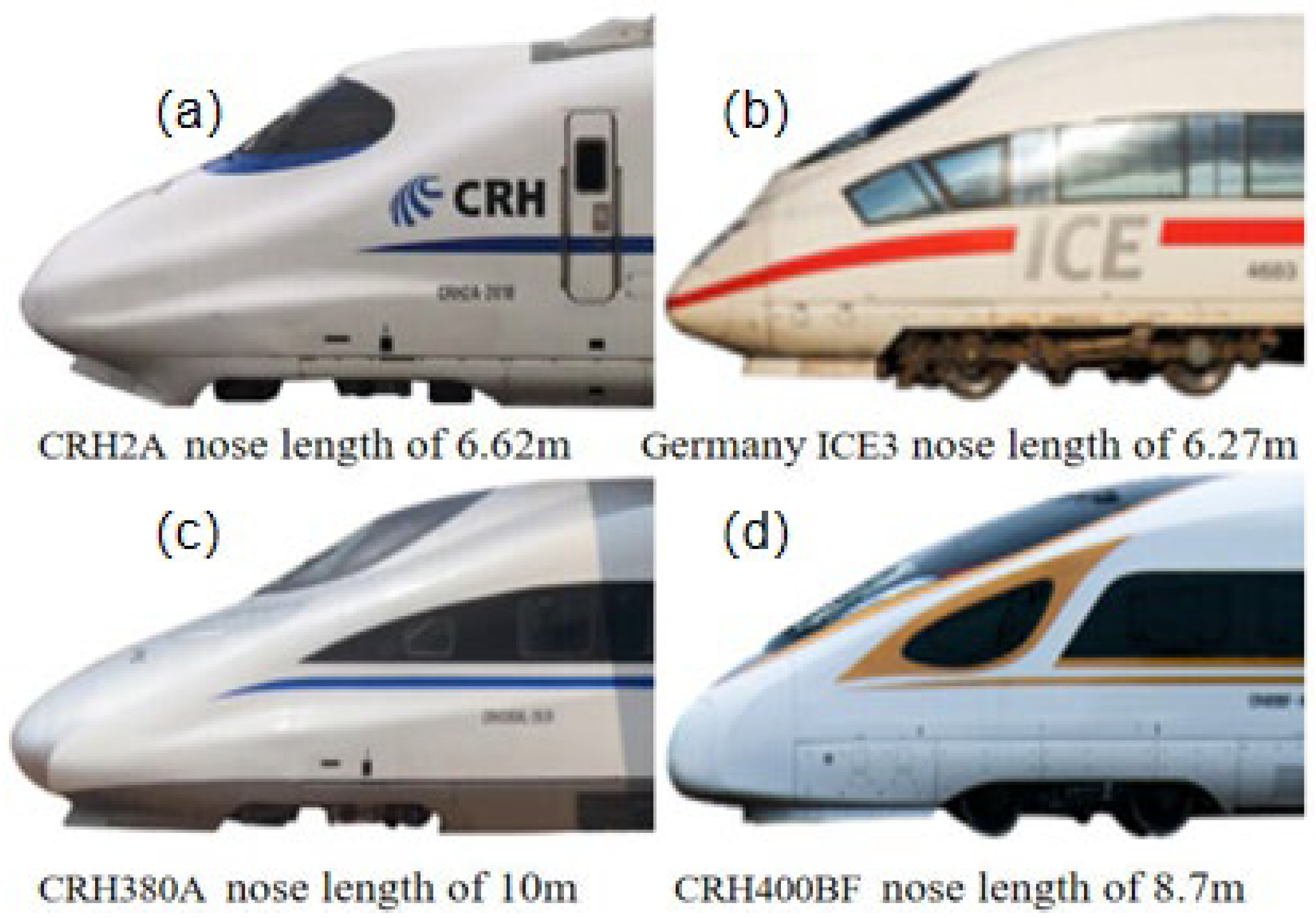
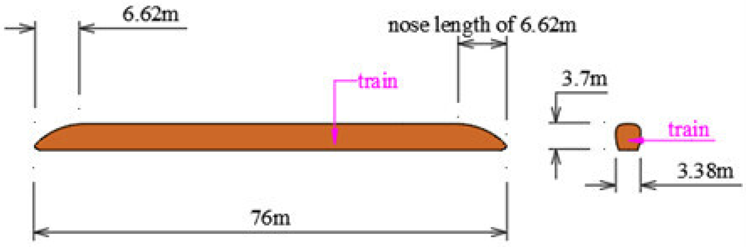
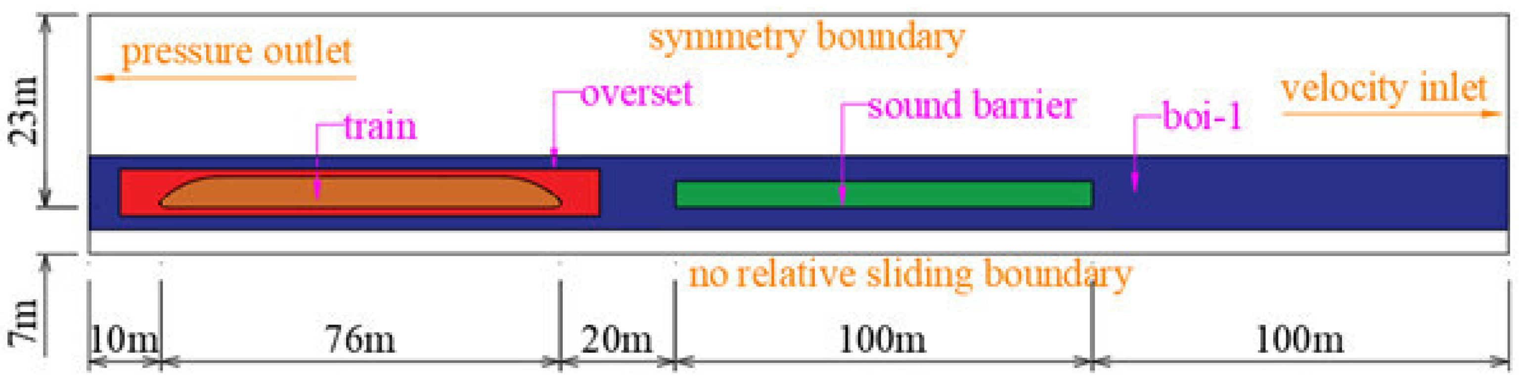
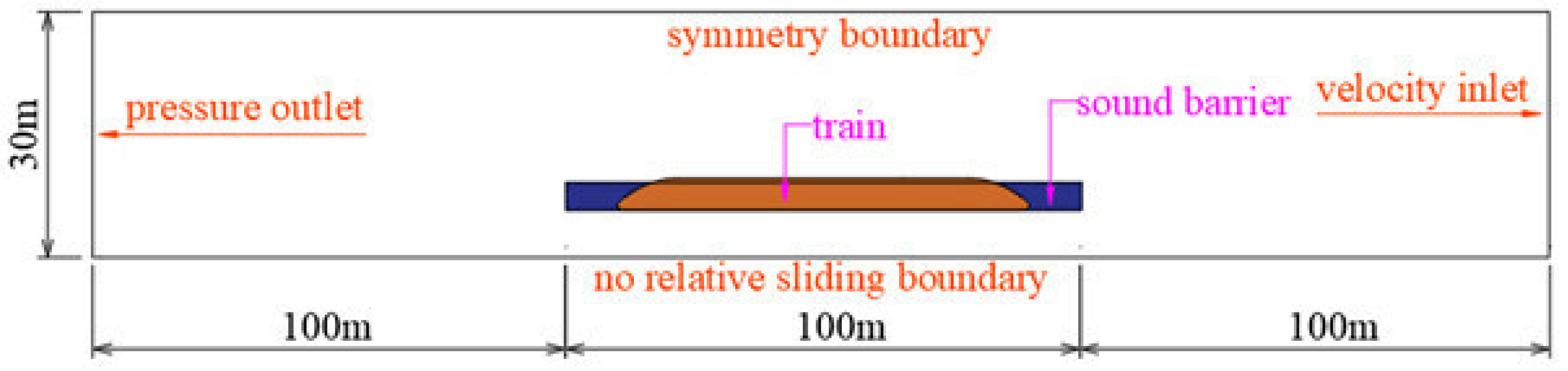
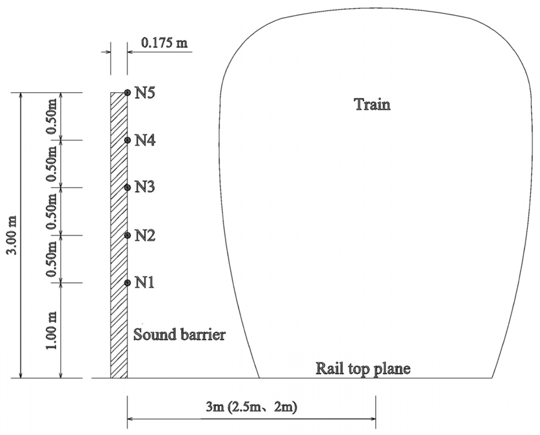
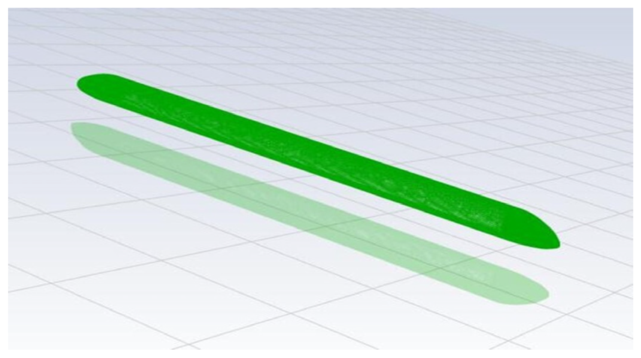
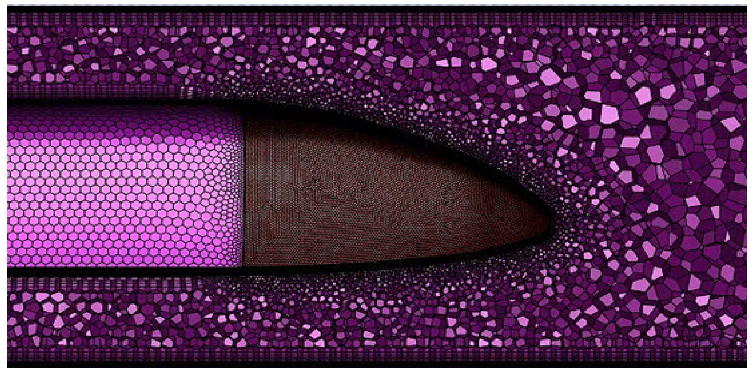
2.1. Train-Sound Barrier Modeling and Meshing

In this study, the high-speed train model was built based on the geometric features of CRH 2A. Previous studies indicate that the aerodynamic characteristics of a 3-car train formation passing through the sound barrier are comparable to those of an 8-car and a 16-car train formation passing through the sound barrier, including the peak wind pressure [25]. Khier et al. and Zhou et al. [26,27] pointed out that the cross-section of the middle region of each train formation remains relatively constant and is situated within a stable flow field region. Hence, in order to minimize computational complexity and enhance efficiency [28], the present numerical simulation employs a three-section train configuration model, comprising a head car, a middle car, and a tail car. The head and tail cars of this train model each have a length of 25.5 m and the middle car is 25 m long, resulting in a total length of 76 m. The cross-sectional width of the train body measures 3.38 m, the height is 3.7 m, and the nose length of both head and tail cars is 6.62 m, as illustrated in Figure 2.

While maintaining the overall aerodynamic characteristics of the train, the modeling approach involves the appropriate simplification of underfloor elements, roof structures, door handles, etc. The modeling excludes subtle components such as bogies, pantographs, and air-conditioning outlets [29], with a focus on smoothing the train’s surface. The head and tail cars, with their relatively complex curved surfaces, are meshed using polyhedral unstructured meshing [28]. The grid control size for the train surface is set at 0.2 m, and grid adaptive technology is applied to refine the local grid on the head and tail cars to 0.05 m, ensuring precision in the calculations. The interface between the train body and the air-fluid field incorporates 20 boundary layers, with the thickness of the first boundary layer set at 0.05 m. The total number of grids in the model amounts to approximately 20 million. Figure 3 and Figure 4 illustrate the grids of the train body model and the dense area around the train head, respectively.

Table 1. The comparison of simulation calculations with different levels of mesh refinement.

Mesh Size of Nose Surface (m)	Peak Positive Pressure of Train Nose (Pa)	Peak Negative Pressure of Train Nose (Pa)
0.02	826	−614
0.05	827	−615
0.08	823	−613

illustrates the comparison of simulation calculations with varying levels of mesh refinement. While all calculation parameters remain constant, the mesh size of the train nose differs with three sizes: 0.02 m, 0.05 m, and 0.08 m. Given the minimal variation observed in simulation results across these three mesh sizes, a mesh size of 0.05 m was selected for the train nose in this study to ensure both calculation effectiveness and accuracy.

2.2. Train-Sound Barrier-Flow Field Transient Calculation Model

In this study, numerical simulations were conducted using the pressure-based solver in ANSYS Fluent software (Ansys 2021 R2) to capture the three-dimensional, viscous, incompressible, and unsteady turbulent airflow. In this transient calculation model, the ground, the surface of the sound barrier, and the train are treated as no-slip wall boundaries, implying no relative sliding between the fluid and these surfaces. The top and both sides of the computational domain are designated as symmetrical wall boundaries. The front side of the computational domain is set as the inlet boundary with a zero flow velocity, while the rear side is specified as the zero-pressure outlet boundary. The dimensions of the computational domain are 306 m in length, 60 m in width, and 30 m in height, as shown in Figure 5.

The moving train model employed the overlapping mesh technique to simulate the dynamic interactions between a train and a sound barrier. This technique is well-suited for non-constant flow problems involving relative motions between multiple objects. It offers the advantage of independent mesh generation, thereby reducing the complexity of mesh generation and computational effort across the entire flow field region. The simulated high-speed train operates at a speed of 360 km/h, corresponding to a Mach number of 0.294. Typically, for fluids with Mach numbers below 0.3, incompressible fluid calculations are simplified, disregarding changes in air density. As a high-speed train traverses a sound barrier, it encounters a three-dimensional, viscous, incompressible, and unstable turbulent air field. Considering these factors, the numerical simulation employs the three-dimensional transient incompressible Navier–Stokes equation and the k-ω turbulence model. The discrete equations were solved in a coupled format, with the pressure term in second-order format, the gradient term in least squares, and the other terms in second-order upwind format. To achieve computational convergence, a minimum residual of 10⁻³ was ensured for each turbulence equation at each time step. The sound barrier in the model has a height of 3 m from the top plane of the track, a thickness of 0.175 m, and a length of 100 m.

2.3. Train-Sound Barrier-Flow Field Steady Calculation Model

In an effort to reduce the computational amount, a steady-state calculation model of the train-sound barrier-external flow field was established, and a comparative analysis was performed to assess the agreement in simulation results between the steady-state model and the transient model. Unlike the transient model, in the steady-state model, the train was entirely within the longitudinal length of the 100 m sound barrier. The meshing methods remain consistent with the transient model. The computational domain has a total length of 300 m, a width of 60 m, and a height of 30 m, as illustrated in Figure 6. The steady-state Navier–Stokes equation in Reynolds time-averaged form and the k-ω turbulence model were employed for the numerical calculation of the model.

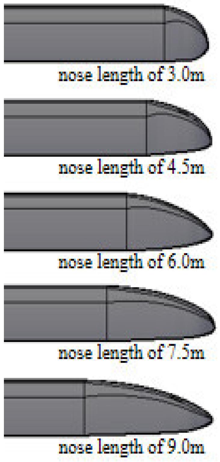
2.4. Parameter Analysis

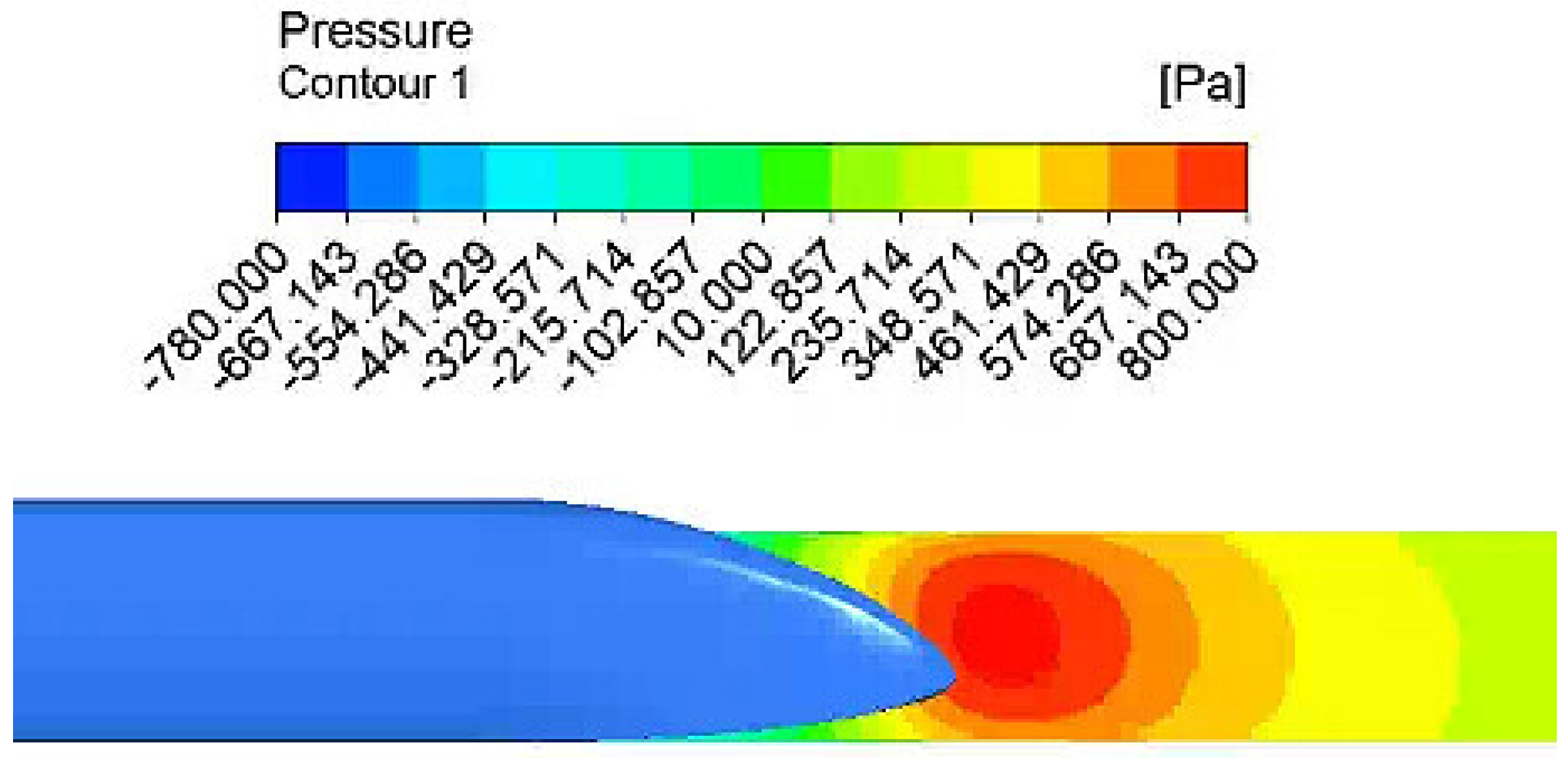
To analyze the distribution characteristics of aerodynamic pressure on the surface of the sound barrier, pressure measurement points were strategically placed in accordance with relevant specifications [30]. In the vertical direction of the sound barrier, measurement points were arranged at intervals of 1.0, 1.5, 2.0, 2.5, and 3.0 m above the bottom of the sound barrier, as shown in Figure 7.

To account for the aerodynamic pressure variations on the surface of the sound barrier arising from different nose lengths and varying distances from the sound barrier to the track centerline, train nose lengths of 3 m, 4.5 m, 6 m, 7.5 m, and 9 m are considered. The specific calculation conditions for each nose length, including distances of 2 m, 2.5 m, and 3 m from the sound barrier to the track centerline, are outlined in

Table 2. Simulation calculation working conditions.

Working Conditions	Sound Barrier–Train Center Distance (m)	Nose Length (m)
1	2.00	3.0, 4.5, 6.0, 7.5, 9.0
2	2.50	3.0, 4.5, 6.0, 7.5, 9.0
3	3.00	3.0, 4.5, 6.0, 7.5, 9.0

.

3. Model Validation

The accuracy of numerical simulation in this study was validated using field test data of aerodynamic pressure on the sound barrier in the Tianjin-Qinhuangdao Passenger Dedicated Line in China from the literature [31]. Employing the aforementioned numerical simulation method, the calculation models corresponding to the field test were established. In this scenario, the CRH 380B high-speed train travels at a speed of 385 km/h, with a distance of 3.4 m between the sound barrier and the center of the train. The simulated peak pressure on the inner surface of the sound barrier was compared with the field test data, and the results are presented in

Table 3. Comparison of in-situ test values and simulated values of aerodynamic pressure.

Measuring Point	Measured Peak (Pa)	Steady-State Simulation		Transient Simulation
		Peak Pressure (Pa)	Relative Error	Peak Pressure (Pa)	Relative Error
219-2	759	737	−2.9%	780	2.8%
230-5	767	742	−3.3%	786	2.5%

. In both transient and steady calculation models, the absolute differences in pressure peak results for two measuring points between numerical simulation and field measurements are below 4%. When the steady-state calculated pressure data is converted from spatial variation to time variation, and compared with the transient pressure curve, as depicted in Figure 8, it becomes evident that the steady-state model and the transient model exhibit substantial consistency in the change of pressure with time. Particularly noteworthy is the close proximity of pressure peaks at the head and tail cars. Figure 9 shows the pressure cloud of the numerically validated simulation model as well as the pressure distribution. Figure 10 shows the time-varying curve of aerodynamic pressure in the in-situ testing. It can be observed that the time variation curve of pressure obtained by numerical simulation closely aligns with the in-situ test results, particularly for the head wave. The peak pressure of the head wave in the numerical simulation closely approximates that observed in the in-situ test. These results affirm that the calculation methods and parameters employed in this study can accurately replicate the actual pressure distribution on the sound barrier [32]. Further parametric analyses can be conducted utilizing the aforementioned CFD modeling method.

4. Results and Discussions

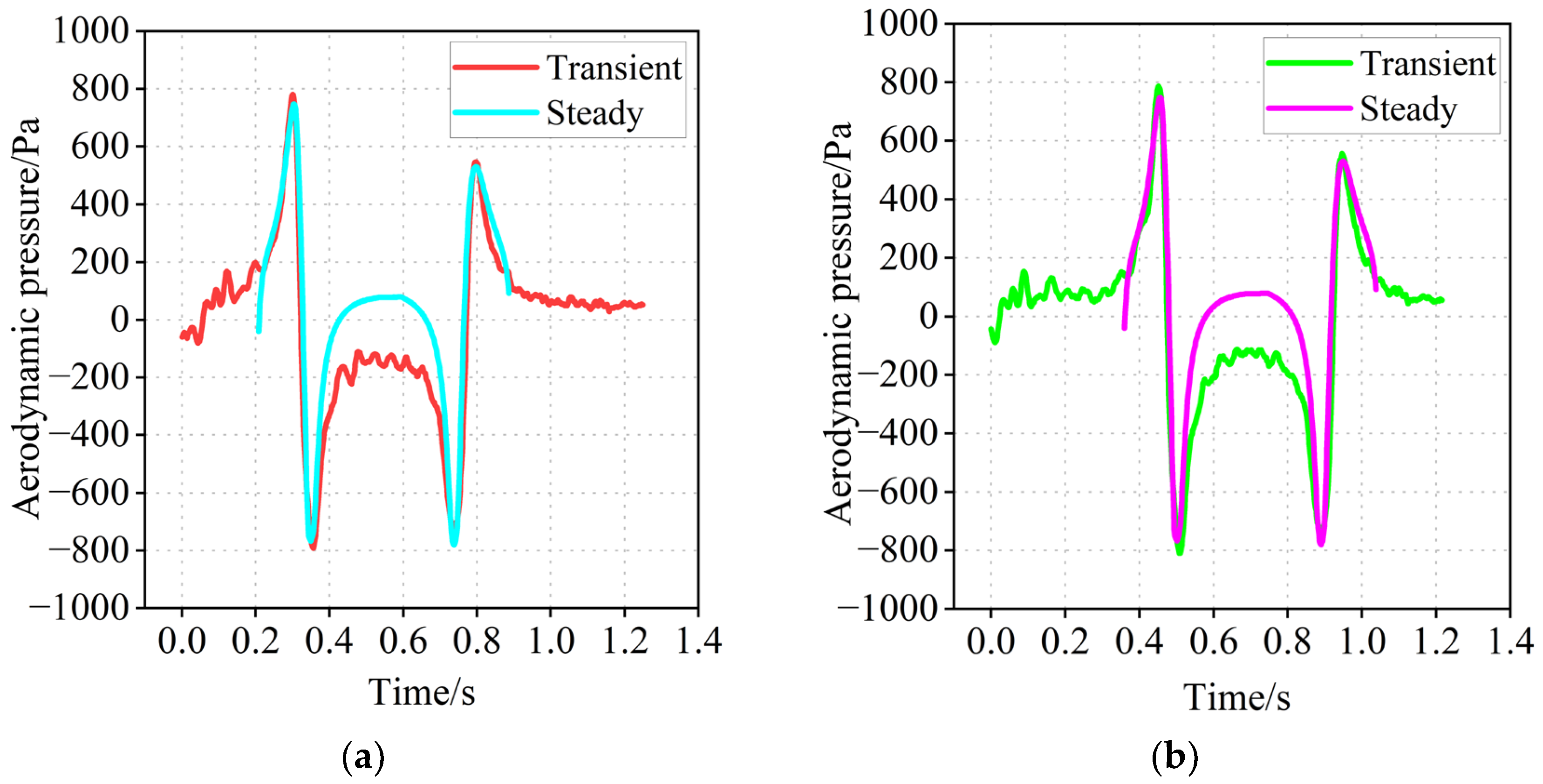
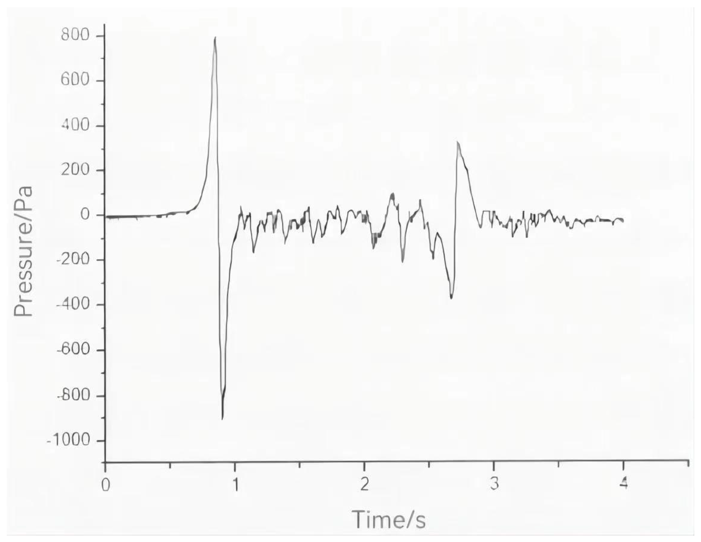
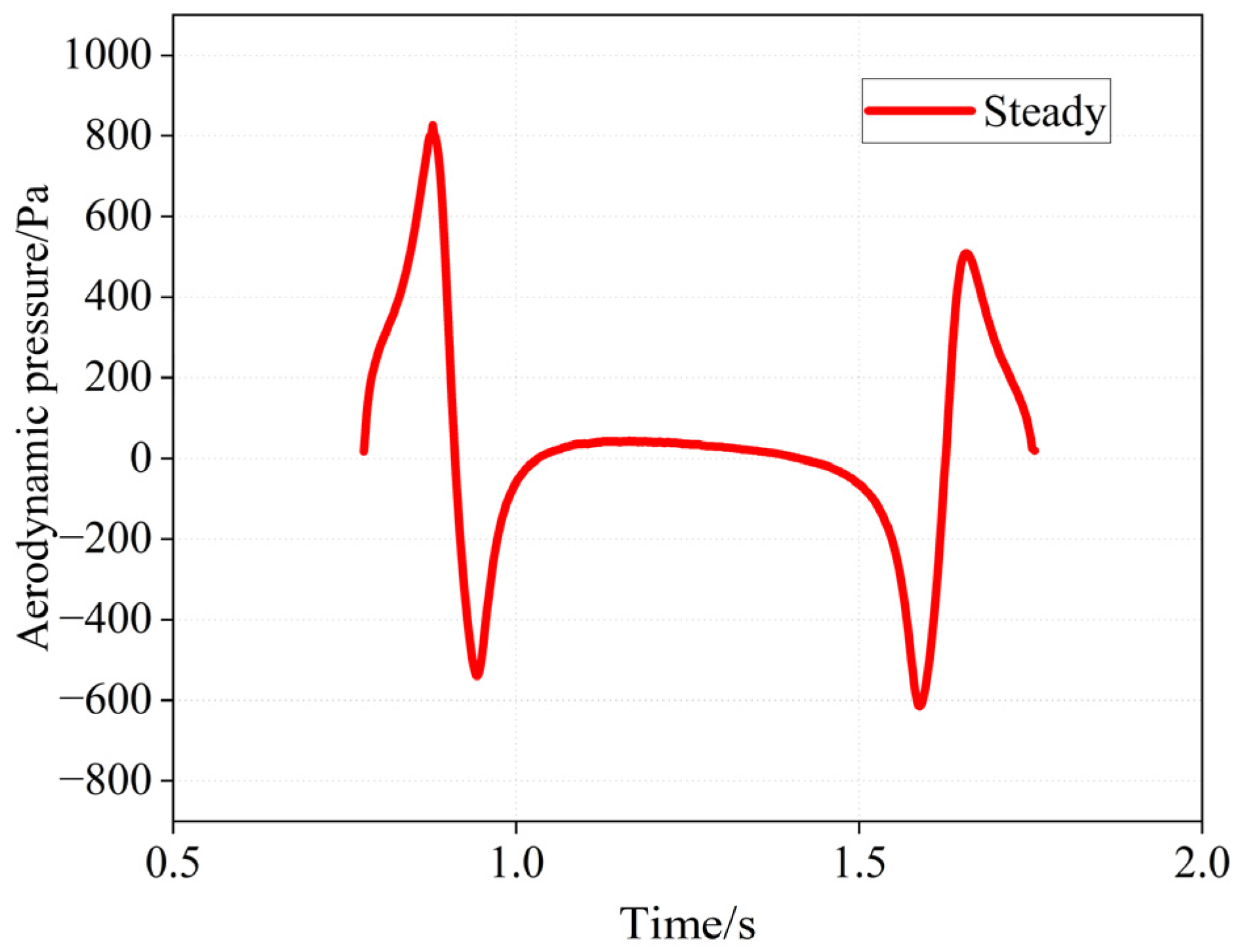
4.1. Basic Characteristics of Pressure Variation on Sound Barrier

Figure 11 depicts the curve representing the distribution of aerodynamic pressure on the inner surface of the sound barrier, measured at a height of 1 m from the top of the track. From the figure, it is apparent that as the train passes this measuring point, there are two distinct aerodynamic pressure changes. In the first pressure fluctuation, a wave peak emerges initially, representing the positive pressure amplitude and indicating that the sound barrier experiences a substantial positive pressure (force from the inside to the outside). This is followed by a trough, indicating the negative pressure amplitude (force from the outside to the inside). Subsequently, the pressure value rises and returns to the initial state. This type of pressure fluctuation is commonly referred to as the “head wave”. The second pressure fluctuation termed the “tail wave” exhibits an opposite pressure change compared to the “head wave”. Specifically, it begins with a negative pressure peak followed by a positive pressure peak. Eventually, the pressure value decreases and returns to the initial state. Notably, the peak value of the head wave is considerably larger than that of the tail wave.

Table 4. The comparison of the peaks of the head and tail waves.

Working Conditions	Peak Head Wave Positive Pressure (Pa)	Peak Tail Wave Negative Pressure (Pa)	Relative Error
ag = 3.0 m, x = 6.0 m	826	−614	34%
ag = 2.5 m, x = 3.0 m	1308	−996	31%

shows a comparison of the peak values of the head and tail waves for the two conditions. The analysis reveals that the peak value of the head wave exceeds that of the tail wave by more than 30%, consistent with findings reported in the literature by Han et al. [25]. Additionally, when the middle carriages pass through the sound barrier, the aerodynamic pressure fluctuation is less pronounced.

4.2. Distribution of Pressure on the Sound Barrier in the Vertical Direction

The peak aerodynamic pressure on the sound barrier varies with different parameters, but the distribution pattern of the peak aerodynamic force along the height direction remains consistent, as illustrated in Figure 12 [33]. The peak aerodynamic pressure is highest at the bottom of the sound barrier, gradually decreasing along the height direction and experiencing a particularly sharp decrease near the top of the sound barrier. This phenomenon is attributed to the smaller effective circulation area of the air at the bottom of the sound barrier compared to that at the top [34,35]. As the air diffuses from the bottom and the middle of the relatively enclosed area into the more open space at the top, it flows out, leading to a sudden change in aerodynamic pressure at the top. Consequently, the peak aerodynamic pressure at the bottom is significantly greater than in the middle and upper regions of the sound barrier.

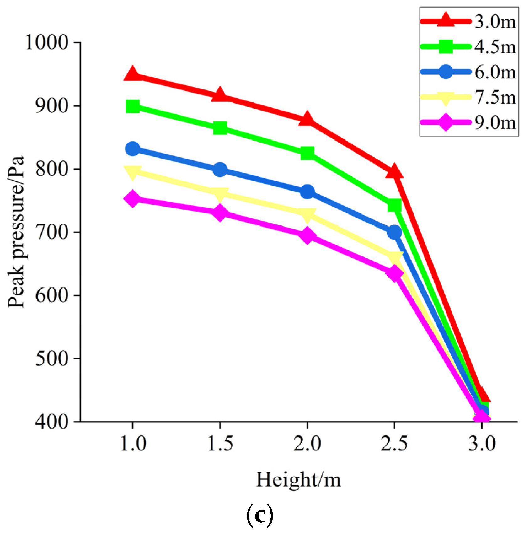
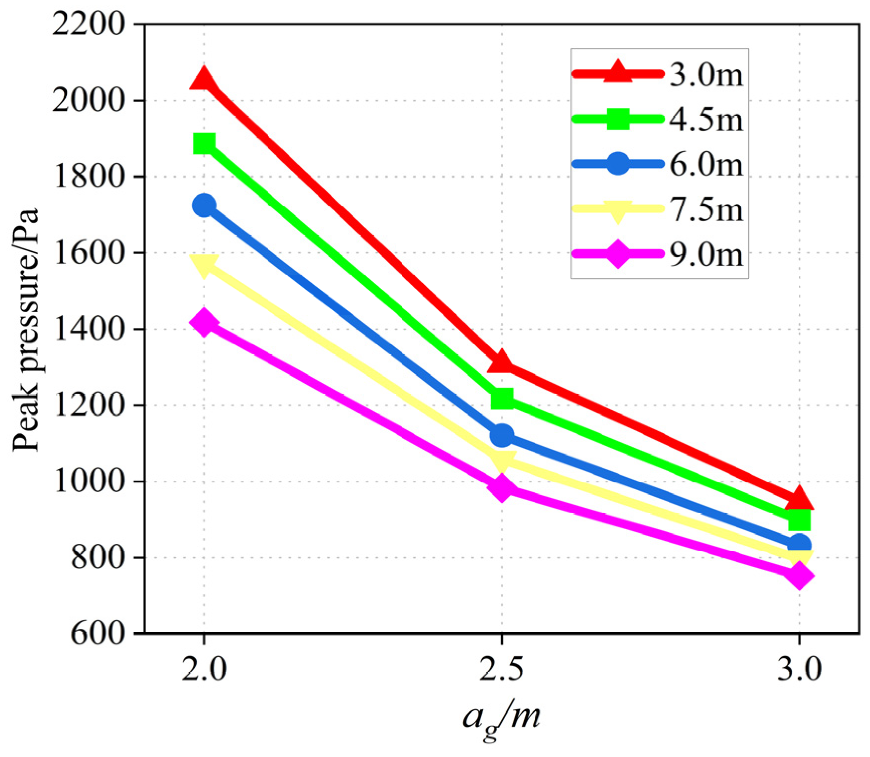
4.3. Influence of Distance to Track Center on Aerodynamic Pressure

Figure 13 illustrates the fluctuation curve of aerodynamic pressure on the sound barrier at various distances from the center of the rail. It is evident that when a high-speed train travels at 360 km/h through a sound barrier, the peak aerodynamic pressure on the surface of the sound barrier diminishes as the barrier moves farther from the railway line’s center. As the length of the train nose extends, ranging from 3.0 m to 9.0 m, and with an increase in the distance between the sound barrier and the center of the rail from 2.0 m to 3.0 m, the aerodynamic pressure peak decreases gradually. When the distance from the center of the rail increases from 2.0 m to 2.5 m, the aerodynamic pressure peak diminishes by 36%, 35%, 35%, 35%, 33%, and 31%, respectively. With an increase in the distance from the center of the rail from 2.5 m to 3.0 m, the aerodynamic pressure peak experiences a decrease of 28%, 26%, 26%, 23%, and 23%, respectively. These findings highlight a non-linear trend in the reduction of aerodynamic pressure peaks on the sound barrier as the distance between the sound barrier and the center of the rail increases. This phenomenon is attributed to the expanding distance between the sound barrier and the train, leading to a more open airflow field and diffusion in the airflow.

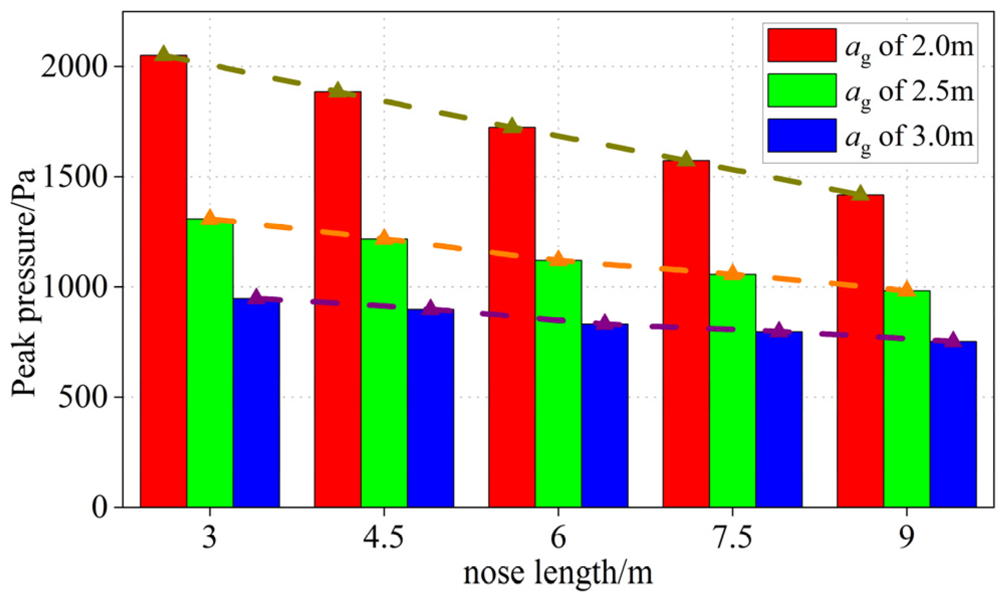
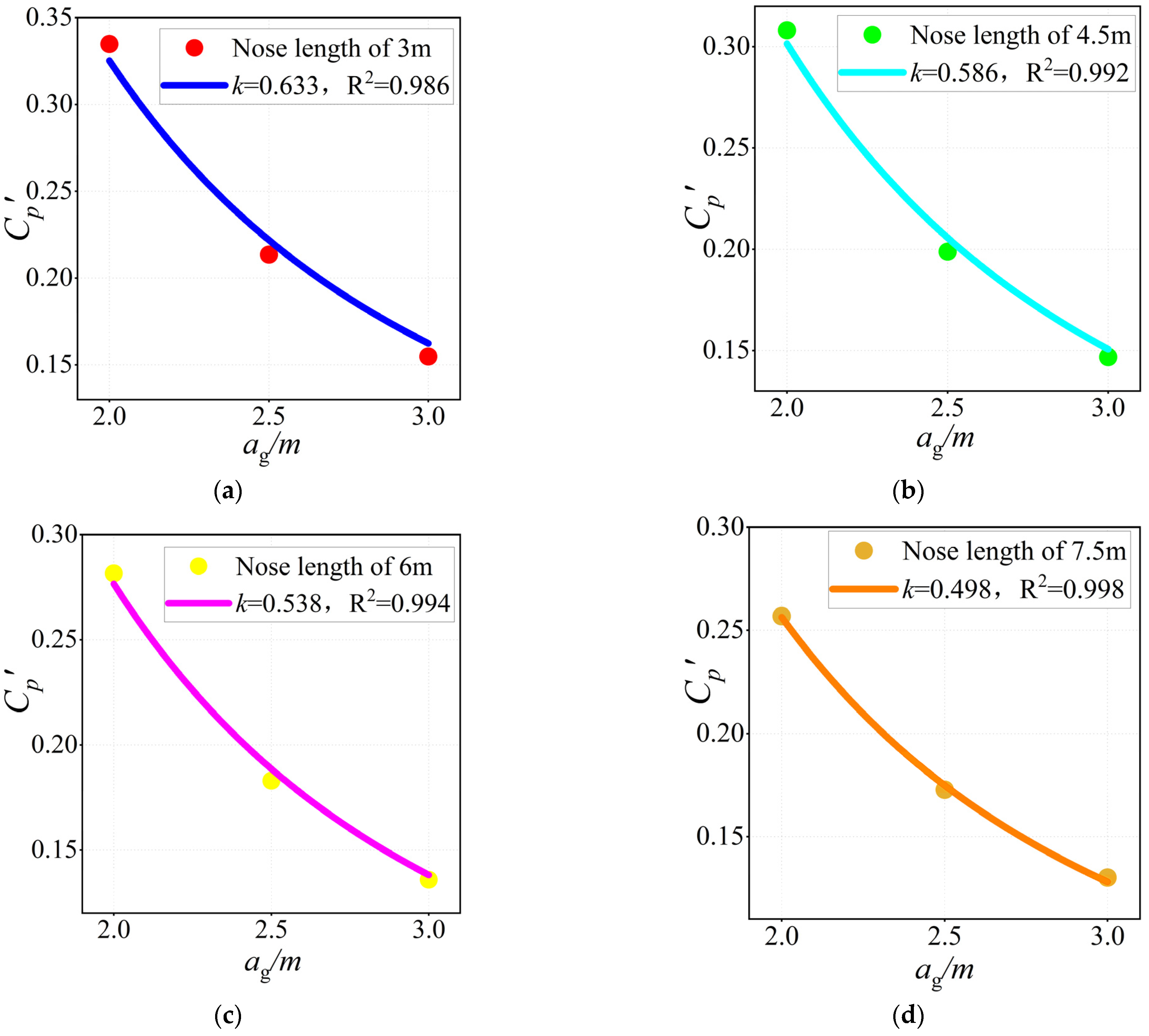
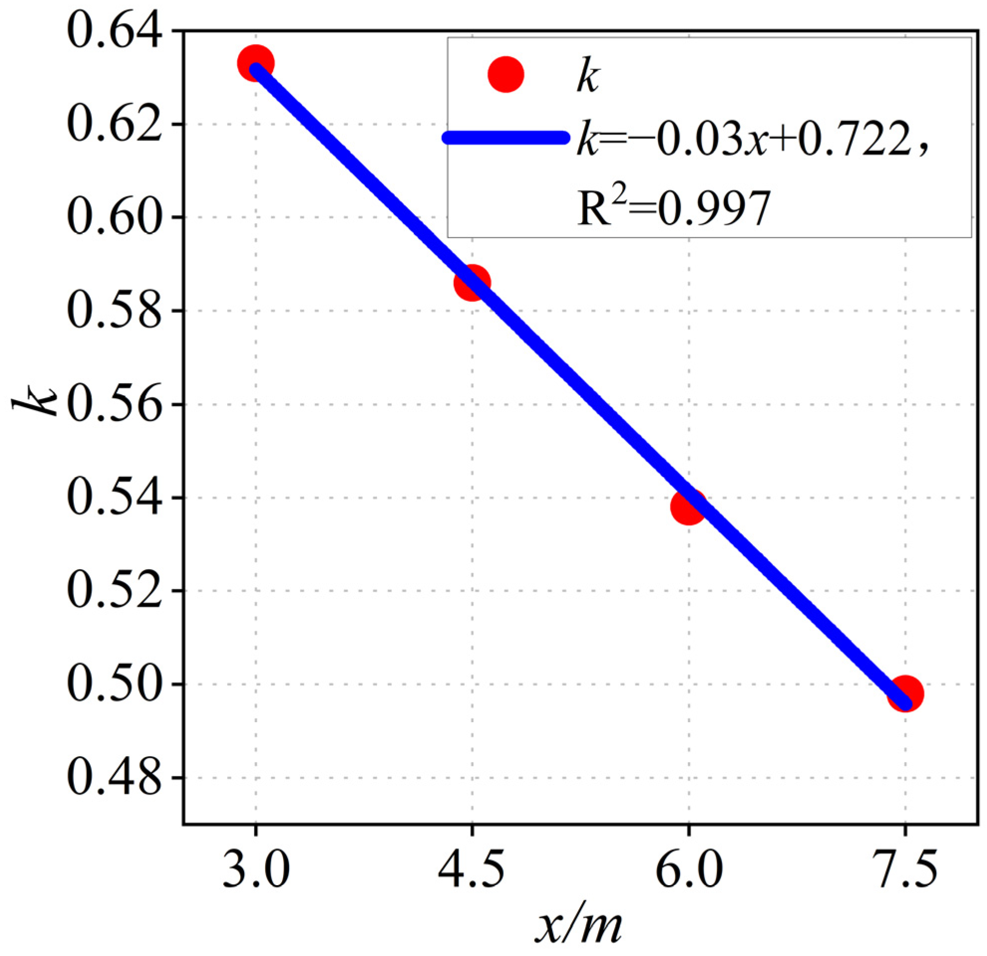
4.4. Effect of Train Nose Length on Aerodynamic Pressure

The nose length of the train refers to the extent of the streamlined section at the head of the train. A streamlined design typically involves shaping the head car to minimize its cross-sectional area, resulting in a smoother profile that leverages aerodynamic principles to decrease air resistance. Previous studies indicate that trains with streamlined noses exhibit superior aerodynamic performance compared to those with square noses [14,36].

Figure 14 illustrates the aerodynamic pressure peaks on surfaces of sound barriers when high-speed trains with varying nose lengths—3 m, 4.5 m, 6 m, 7.5 m, and 9 m—pass through at distances of 2 m, 2.5 m, and 3 m from the center of the railway track. The comparison reveals that, for a given distance from the sound barrier to the track center, the peak pressure on the sound barrier decreases with increasing train nose length. When the distances between the sound barrier and the train’s center are considered to be 2.0 m, 2.5 m, and 3.0 m, respectively, increasing the nose length from 3 m to 9 m will result in peak aerodynamic pressure decreases of 31%, 25%, and 21% on the surface of the sound barrier. This indicates that nose length has a significant effect on the peak aerodynamic pressure on the surface of the sound barrier caused by the running trains. As shown in Figure 15, different lengths of train noses result in varying rates of change in the cross-sectional area along the surface of the train head. The maximum rate of change occurs in the head section with a 3 m nose length, while the minimum rate of change occurs with a 9 m nose length. This streamlined difference leads to reduced air resistance during the travel of the train with a 9 m nose length, resulting in weaker aerodynamic pressure effects on the surface of the sound barrier. This is why trains with longer noses generate smaller aerodynamic pressures when passing through sound barriers.

At present, some standards [37] utilize the following calculation model to determine the aerodynamic pressure on the vertical noise barrier caused by high-speed trains, as depicted in Equations (1) and (2).

$$p_{\mathrm{k}}=\frac{\rho v_{\mathrm{t}\mathrm{r}}^2}{2}·k·C_P$$

(1)

$$C_P=\frac{2.5}{{\left(a_{\mathrm{g}}+0.25\right)}^2}+0.02$$

(2)

where p_k is the characteristic value of distributed load (Pa), ρ is the air density taken as 1.225 kg/m³, v_tr is the train speed (m/s), C_p is the air pressure coefficient, k is the train shape coefficient, and a_g is the distance between sound barrier and train center (m). To eliminate the influence of speed, the pressure values are normalized according to Equation (3). The disparity between C_p and C_p’ lies in the fact that C_p’ represents the actual aerodynamic pressure coefficient, accounting for the train’s shape. The C_p’ values induced by high-speed trains with various nose lengths (3 m, 4.5 m, 6 m and 7.5 m) at different distances are presented in

Table 5. The C_p’ values induced by high-speed trains with various nose lengths at different distance.

ag (m)	Nose Length of 3.0 m	Nose Length of 4.5 m	Nose Length of 6.0 m	Nose Length of 7.5 m
2.00	0.3281	0.3019	0.2760	0.2516
2.50	0.2092	0.1948	0.1793	0.1692
3.00	0.1516	0.1438	0.1331	0.1275

.

$$p_{\mathrm{k}}=\frac{\rho v_{\mathrm{t}\mathrm{r}}^2}{2}\cdot C_P\mathrm{’}$$

(3)

Based on the C_p’ values provided above and the correlation between the aerodynamic pressure coefficient and distance, as illustrated in Equation (2), the corresponding k values for high-speed trains with different nose lengths can be determined, as depicted in Figure 16. It can be observed that as the nose length increases, the train shape coefficient gradually decreases. Figure 17 exhibits the changing trend of the train shape coefficient in relation to the nose length of the train, demonstrating an excellent linear relationship between the two parameters with a coefficient of determination of 0.997. Consequently, a calculation formula for the train shape coefficient, considering the effect of nose length, was established, as shown in Equation (4). By integrating Equations (1) and (2), a calculation model for aerodynamic pressure on sound barriers, considering the influence of the nose length of high-speed trains, was derived, as presented in Equation (5).

Table 6. The comparison of simulation pressure values and the pressure calculated using Equation (5).

Working Conditions	Simulated Value (Pa)	Calculated Value by Equation (5) (Pa)	Relative Error
ag = 2.0 m, x = 6.0 m	1725	1706	1.1%
ag = 3.0 m, x = 7.5 m	797	781	2.0%
ag = 2.5 m, x = 9.0 m	983	971	1.2%

shows the comparison between the simulation peak pressure values and the peak pressure calculated using Equation (5). It demonstrates that the two sets of data exhibit close agreement, providing further evidence of the effectiveness of the proposed formula.

$$k=-0.03x+0.722$$

(4)

$$p_{\mathrm{k}}=\frac{\rho v_{\mathrm{t}\mathrm{r}}^2}{2}\cdot \left(-0.03x+0.722\right)\cdot \left[\frac{2.5}{{\left(a_{\mathrm{g}}+0.25\right)}^2}+0.02\right]$$

(5)

where x is the nose length (m). To validate the accuracy of the proposed pressure equation, a dataset not utilized in constructing the pressure model in this article was employed. Specifically, with a train nose length of 9 m and a distance of 2 m between the sound barrier and the train center, the calculated peak aerodynamic pressure is 1422 Pa, closely aligning with the original value of 1418 Pa, resulting in a relative error of 0.28%.

5. Conclusions

In this study, the aerodynamic pressure on sound barriers induced by high-speed trains was computed using CFD simulations. Through a comparison between the simulation results and field measurements extracted from the literature, it was observed that there was a notable concurrence in the peak pressure data and development with time, indicating the efficacy of the simulation method. Subsequently, the essential characteristics of pressure variation on sound barriers and pressure distribution along the vertical direction were explored. Additionally, the impact of distance to the train center and the train nose length on aerodynamic pressure on sound barriers was analyzed. The following conclusions were drawn:

(1)

When a high-speed train passes through the sound barrier, it produces obvious “head wave” and “tail wave” effects, and the peak value of the “head wave” is obviously larger than the peak value of the “tail wave”; in the vertical direction of the sound barrier, the pressure reaches the peak value at the bottom, decreases gradually from the bottom to the top, and decreases rapidly when it is near the top of the sound barrier.

(2)

As the distance between the sound barrier and the center of the train gradually increases, the peak aerodynamic pressure on the surface of the sound barrier gradually decreases, showing a non-linear development trend.

(3)

The nose length has a great influence on the aerodynamic force of the sound barrier, the aerodynamic pressure generated by a train with a long nose length is smaller than that of a train with a short nose length, and the formula for calculating the aerodynamic pressure generated by a high-speed train on the sound barrier with respect to the nose length has been established.

This study focuses solely on the distribution of aerodynamic pressure on vertical sound barriers when a train passes. A limitation is that it does not address other types of sound barriers, such as semi-enclosed or fully enclosed sound barriers.

References

1. Mellet, C.; Letourneaux, F.; Poisson, F.; Talotte, C. High speed train noise emission: Latest investigation of the aerodynamic/rolling noise contribution. J. Sound Vib. 2006, 293, 535–546. [Google Scholar] [CrossRef]
2. Kitagawa, T.; Nagakura, K. Aerodynamic noise generated by shinkasnsen cars. J. Sound Vib. 2000, 231, 913–924. [Google Scholar] [CrossRef]
3. Jean, P. The effect of structural elasticity on the efficiency of noise barriers. J. Sound Vib. 2000, 237, 1–21. [Google Scholar] [CrossRef]
4. Liu, W. Simulation Research of Aerodynamic Load on Sound Barrier of High-Speed Railway. Master’s Thesis, Beijing Jiaotong University, Beijing, China, 2014; pp. 3–12. [Google Scholar]
5. Kikuchi, K.; Maeda, T.; Yanagizawa, M. Numerical simulation of the phenomena due to the passing-by of two bodies using the unsteady boundary element method. Int. J. Numer. Methods Fluids 1996, 23, 445–454. [Google Scholar] [CrossRef]
6. Rong, X.; Chen, X. Aerodynamic characterization of high-speed trains and its development. J. China Railw. Soc. 1998, 20, 128–133. [Google Scholar]
7. Li, H.; Xuan, Y.; Wang, L.; Li, Y.; Fang, X.; Shi, G. Research on numerical simulation of high-speed railway noise barrier aerodynamic pressure. Appl. Mech. Mater. 2013, 274, 45–48. [Google Scholar] [CrossRef]
8. Luo, C.; Zhou, D.; Chen, G.; Krajnovic, S.; Sheridan, J. Aerodynamic effects as a maglev train passes through a noise barrier. Flow Turbul. Combust. 2020, 105, 6–7. [Google Scholar] [CrossRef]
9. Bi, R.; Li, X.; Zheng, J.; Hu, Z.; Xu, H.; Li, S. Characteristics of aerodynamic pressure of vertical sound barriers on high speed railway bridge at 400 km/h. China Railw. Sci. 2021, 42, 68–77. [Google Scholar]
10. Shi, Z.; Yang, S.; Pu, Q.; Deng, L. Study on the characteristic of aerodynamic load on sound barriers by 350-400km/h high-speed trains. China Railw. Sci. 2018, 39, 103–111. [Google Scholar]
11. Kang, J.; Li, R. Fatigue performance analysis of sound barrier under aerodynamic pressure of high-speed train. Mech. Eng. Autom. 2016, 1, 23–25. [Google Scholar]
12. Chen, X.; Li, S.; Wang, Z. Numerical simulation study on high-speed train induced impulsive pressure on railway noise barrier based on ALE. J. China Railw. Soc. 2011, 33, 21–26. [Google Scholar]
13. Scholz, M.; Buba, Z.; Boruttau, M. Consulting Report: Noise Barrier for High Speed Railway; Germany Planning Engineering Consulting+ Services Ltd.: Beijing, China, 2006. [Google Scholar]
14. Schetz, J. Aerodynamics of high-speed trains. Annu. Rev. Fluid Mech. 2001, 53, 371–414. [Google Scholar] [CrossRef]
15. Belloli, M.; Pizzigoni, B.; Ripamonti, F.; Rocchi, D. Fluid-structure interaction between trains and noise-reduction barriers numerical and experimental analysis. WIT Trans. Built Environ. 2009, 105, 49–60. [Google Scholar]
16. Lv, M.; Li, Q.; Ning, Z.; Ji, Z. Study on the aerodynamic load characteristic of noise reduction barrier on high-speed railway. J. Wind. Eng. Ind. Aerod. 2018, 176, 254–262. [Google Scholar]
17. Zou, Y.; Fu, Z.; He, X.; Cai, C.; Zhou, J.; Zhou, S. Wind load characteristics of wind barriers induced by high-speed trains based on field measurements. Appl. Sci. 2019, 9, 4865. [Google Scholar] [CrossRef]
18. Rocchi, D.; Tomasini, G.; Schito, P.; Somaschini, C. Wind effects induced by high speed train pass-by in open air. J. Wind. Eng. Ind. Aerod. 2018, 173, 279–288. [Google Scholar] [CrossRef]
19. MacNeill, R.A.; Holmes, S.; Lee, H.S. Measurement of the aerodynamic pressure produced by passing trains. In Proceedings of the IEEE/ASME Joint Railroad Conference, Washington, DC, USA, 4–6 April 2002; pp. 57–64. [Google Scholar]
20. Paz, C.; Suárez, E.; Gil, C. Numerical methodology for evaluating the effect of sleepers in the underbody flow of a high-speed train. J. Wind. Eng. Ind. Aerod. 2017, 167, 140–147. [Google Scholar] [CrossRef]
21. Dr. White CRH2A-2010 out of Nanjing Station toward Linchang. Available online: https://www.bilibili.com/video/av20644660/?redirectFrom=h5 (accessed on 11 March 2018).
22. After Ulm—Going Global (Part II). Available online: https://www.puxiang.com/galleries/74d6ec9b558fa4bc8907510008088e81 (accessed on 25 November 2019).
23. CRH380AL out of Shenzhen North Station. Available online: https://www.bilibili.com/video/BV1Ms4y1z7TT/ (accessed on 20 May 2023).
24. CRH400BF. Available online: https://tuchong.com/2694859/ (accessed on 11 November 2017).
25. Han, J.; Xiao, X.; He, B.; Zhou, X.; Jin, X. Study on dynamic characteristics of different forms of sound barriers. J. Mech. Eng. 2013, 49, 20–27. [Google Scholar] [CrossRef]
26. Khier, W.; Breuer, M.; Durst, F. Flow structure around trains under side wind conditions: A numerical study. Comput. Fluids, 2000; 29, 179–195. [Google Scholar]
27. Zhou, D.; Tian, H.; Lu, Z. Effects of high wind on the aerodynamic performance of passenger trains running on embankments. J. China Railw. Soc. 2007, 7, 6–9. [Google Scholar]
28. Li, X.; Yang, Z.; Zhang, J.; Zhang, W. Aerodynamics properties of high-speed train in strong wind. J. Traffic Transp. Eng. 2009, 9, 66–73. [Google Scholar]
29. Zhang, L.; Zhang, J.; Zhang, W. Fluid-solid coupling vibration response analysis of high-speed train passing through sound barrier. J. Dyn. Control 2014, 12, 153–159. [Google Scholar]
30. TB/T 3503.4-2018; National Railway Administration of the People’s Republic of China: Aerodynamics for Railway Applications Part 4: Specification for Numerical Simulation of Train Aerodynamic Performance. China Railway Press: Beijing, China, 2018.
31. Shi, M. Experimental Study on Aerodynamic Loading Characteristics of High-Speed Railroad Sound Barriers. Master’s Thesis, Beijing Jiaotong University, Beijing, China, 2015; pp. 61–67. [Google Scholar]
32. Meng, S.; Zhou, D.; Xiong, X.; Chen, G. The effect of the nose length on the aerodynamics of a high-speed train passing through a noise barrier. Flow. Turbul. Combust. 2022, 108, 411–431. [Google Scholar] [CrossRef]
33. Luo, W.; Li, H. Analysis of dynamic response of sound barrier under aerodynamic load. Noise Vib. Control. 2016, 36, 162–165. [Google Scholar]
34. Wu, X.; Zhu, Y.; Xian, L.; Huang, Y.; Du, P. Numerical study on dynamic characteristics of Y-type sound barriers for high-speed railroads. J. Cen. South. Univ. 2022, 53, 737–746. [Google Scholar]
35. Long, L.; Zhao, L.; Liu, L. Aerodynamic study of train-induced acoustic barrier structures. Eng. Mech. 2010, 27, 246–250. [Google Scholar]
36. Lv, J. Research on High-Speed Railroad Plug-in Plate and Integral Sound Barrier Structure. Ph.D. Thesis, Southeast University, Nanjing, China, 2010; pp. 46–47. [Google Scholar]
37. EN 14067-4; Railway Applications-Aerodynamics-Part 4: Requirements and Test Procedures for Aerodynamics on Open Track. European Committee for Standardization: Brussels, Belgium, 2005.
Figure 1. Nose lengths of different high-speed trains: (a) CRH 2A [21]; (b) Germany ICE 3 [22]; (c) CRH 380A [23]; (d) CRH 400BF [24].
Applsci 14 02898 g001
Figure 2. CRH 2A geometric parameters.
Applsci 14 02898 g002
Figure 3. Body model.
Applsci 14 02898 g003
Figure 4. Area of grid densification at the head car of the train.
Applsci 14 02898 g004
Figure 5. Modeling of transient calculation.
Applsci 14 02898 g005
Figure 6. Overall model for steady-state calculations.
Applsci 14 02898 g006
Figure 7. Train and sound barrier location and measurement points.
Applsci 14 02898 g007
Figure 8. Comparison of steady-state and transient aerodynamic pressure curves: (a) First measurement point “219-2”; (b) Second measurement point “230-5”.
Applsci 14 02898 g008
Figure 9. The simulation results and the pressure distribution.
Applsci 14 02898 g009
Figure 10. Time-varying curve of aerodynamic pressure at 385 km/h speed [31].
Applsci 14 02898 g010
Figure 11. The curve of the distribution of aerodynamic pressure on the inner surface of the sound barrier.
Applsci 14 02898 g011
Figure 12. Change curve of peak aerodynamic pressure under different working conditions: (a) Distance to track center is 2 m; (b) Distance to track center is 2.5 m; (c) Distance to track center is 3 m.
Applsci 14 02898 g012aApplsci 14 02898 g012b
Figure 13. Variation curves of peak aerodynamic pressure for different sound barrier–train center distances.
Applsci 14 02898 g013
Figure 14. Variation of aerodynamic pressure peak values for different nose lengths.
Applsci 14 02898 g014
Figure 15. Heads with different nose lengths.
Applsci 14 02898 g015
Figure 16. Fitted curves of ag and Cp’ for different nose length conditions: (a) Nose length of 3 m; (b) Nose length of 4.5 m; (c) Nose length of 6 m; (d) Nose length of 7.5 m.
Applsci 14 02898 g016
Figure 17. Fitted curve of k and nose length.
Applsci 14 02898 g017