Time of Flight Distance Sensor–Based Construction Equipment Activity Detection Method

Abstract

In this study, we delve into a novel approach by employing a sensor-based pattern recognition model to address the automation of construction equipment activity analysis. The model integrates time of flight (ToF) sensors with deep convolutional neural networks (DCNNs) to accurately classify the operational activities of construction equipment, focusing on piston movements. The research utilized a one-twelfth-scale excavator model, processing the displacement ratios of its pistons into a unified dataset for analysis. Methodologically, the study outlines the setup of the sensor modules and their integration with a controller, emphasizing the precision in capturing equipment dynamics. The DCNN model, characterized by its four-layered convolutional blocks, was meticulously tuned within the MATLAB environment, demonstrating the model’s learning capabilities through hyperparameter optimization. An analysis of 2070 samples representing six distinct excavator activities yielded an impressive average precision of 95.51% and a recall of 95.31%, with an overall model accuracy of 95.19%. When compared against other vision-based and accelerometer-based methods, the proposed model showcases enhanced performance and reliability under controlled experimental conditions. This substantiates its potential for practical application in real-world construction scenarios, marking a significant advancement in the field of construction equipment monitoring.

1. Introduction

To improve the reliability of productivity estimation and evaluation in construction projects, it is critical to thoroughly understand and monitor the operational activities of various equipment [1]. Analyzing the history of equipment activity provides valuable information that can be integrated into construction simulation models [2,3,4]. This integration allows for a quantitative evaluation of a project’s performance, enhancing the accuracy of productivity assessments. However, traditional manual techniques for analyzing activity, such as timing work with stopwatches or determining activity duration from recorded video, are notably labor-intensive [1,2]. These methods become particularly impractical for long-term data analysis, where they are prone to introducing significant costs and potential errors in data classification [5]. Consequently, such methods are often deemed unsuitable for accurate and efficient productivity evaluation. Recently, researchers have been trying to solve this problem by incorporating experimentally determined weights into established productivity estimation and evaluation methods based on empirical data [6]. Methods for recognizing construction equipment activity can be broadly classified into two main categories [7].

The first category employs vision-based methods, using images or videos to identify and analyze equipment activities. In vision-based methods, artificial intelligence and computer vision technologies are utilized to analyze 2D images or videos as the primary training data. These methods enable object detection and semantic/instance segmentation [8,9]. The second category relies on measurement sensors, utilizing data from various sensors to monitor and interpret equipment activities. Notable methodologies encompass the deployment of acoustic sensors (e.g., microphones) [10,11], inertial measurement units (IMUs), integrating gyroscopes, accelerometers, and magnetometers [12,13], global positioning systems (GPSs) [14], ultra-wideband (UWB) technologies [15], and radio frequency identification (RFID) systems [15]. Among these technologies, acoustic sensors (e.g., microphones) demonstrate limitations in isolating equipment-specific signals within environments laden with obstacles and ambient noise [12].

A significant issue discussed in the context of the vision-based method is that the learning data are greatly influenced by weather, light, and shadows, and even the direction in which the object is observed and the color of the object can significantly affect the recognition results. On the other hand, in the sensor-based method, since the sensor’s measurements are directly used for learning, there is a problem in that differences in activity recognition results can occur even when applying the same system if there are differences in the size or shape of the equipment. Accordingly, this study conducts research on the sensor-based method and has developed a data-handling approach and an artificial intelligence-based activity recognition model to solve the problems associated with this methodology.

The composition of each section is as follows:

Section 2: The discussion centers on reviewing existing studies within two distinct categories that are instrumental for the recognition of construction equipment activities. This review not only unpacks the most current trends but also delves into the limitations inherent in these methodologies. Additionally, this chapter sheds light on the fundamental concepts of optimization algorithms, which play a pivotal role in the realm of artificial intelligence training.

Section 3: The focus shifts to elaborating the configuration of the data acquisition system. This system has been meticulously applied to both defined excavator activities and a one-twelfth scale model, specifically tailored for experimental purposes. Furthermore, this section provides a comprehensive overview of the strategies employed for the handling and analysis of the collected data. The DCNN model developed for the quantitative analysis of these data is presented in detail, highlighting the intricacies of each layer within every stage and outlining the configurations of the hyperparameters utilized in the experiments.

Section 4: An interpretation of sample images for each data class inputted into the model is offered, alongside a presentation of the model’s training and validation outcomes. These outcomes are meticulously delineated through confusion matrices and assessments of the model’s precision, recall, and accuracy. The practicability of the proposed methodology is evaluated through a comparative analysis with both vision-based and sensor-based models. By building upon the analysis of the results, this chapter further explores the research’s contributions and limitations, setting the stage for the proposition of directions for future research endeavors.

Section 5: A concise summary of the key results and discoveries emanating from the research is provided, encapsulating the essence and significant achievements of the study.

2. Literature Review and Background

This section reviews the research on identifying equipment operations based on visual data (using images or videos) and the research based on non-visual data (using measurement sensors). Additionally, the study introduces adaptive moment estimation (Adam) optimization, which is used in the convolutional model.

2.1. Vision-Based Method for Recognizing Equipment Activity

Vision-based methods have emerged as a cornerstone for recognizing and monitoring construction equipment activities through the use of image and video data. These techniques leverage advanced computer vision technologies such as convolutional neural networks (CNNs) for spatial feature analysis and support vector machines (SVMs) for classification tasks. The deployment of the histogram of oriented gradients (HOG) features in conjunction with SVM classifiers has proven effective in identifying earthmoving equipment activity [16,17]. Furthermore, the application of 3D convolutional neural networks (3D CNNs) underscores the progression in capturing the spatial and temporal dynamics of construction activities through video analysis [7,18]. Recent advancements include the integration of CNN with long short-term memory (LSTM) networks, presenting a hybrid model adept at capturing the sequential nature of construction equipment activities. This approach addresses the temporal complexities inherent in these operations, marking a significant leap in accurately predicting the actions of construction machinery [19].

Despite their benefits, vision-based methods encounter significant challenges. These include obstructions by adverse weather conditions (e.g., fog, dust, rain, and snow), unfavorable lighting conditions (e.g., luminous flux, illuminance, beam angle, and color temperature), and occlusions by construction equipment, which can significantly impair activity recognition [20,21]. For example, poor lighting and occlusions have been identified as factors that may lead to inaccurate activity detection and classification [22]. The necessity for extensive labeled data for training deep learning models further adds to the complexity and cost of system implementation. The high computational demand for processing and analyzing video data in real time presents another hurdle, limiting the practicality of these methods on construction sites. This challenge is exacerbated by the need for powerful computing hardware to effectively implement complex deep learning models. Moreover, the capture of video data on construction sites raises privacy concerns, highlighting the importance of implementing robust privacy measures to mitigate potential issues [1,23].

2.2. Sensor-Based Method for Recognizing Equipment Activity

Sensor-based methods enable the monitoring of construction equipment by analyzing the location and movement data collected from sensors attached to the machinery. These methods can be defined as real-time location system (RTLS) methods and kinematic methods. In RTLS research, sensors such as GPS, UWB, and RFID have been used to analyze the information (trajectories and regions) of construction equipment by combining it with the site’s geographical information, thereby estimating the equipment’s productivity [24,25,26,27,28,29]. However, RTLS methods rely solely on location information, which presents limitations in estimating work productivity based on the detailed actions of the equipment. In order to overcome this, kinematic method-based activity estimation approaches have been researched, applying sensors such as accelerometers and IMUs to directly measure the equipment’s movement.

Studies have been conducted on attaching accelerometers (smartphones) to the cabin’s control panel to use acceleration information for classifying the specific activities of equipment and extracting cycle times [5,29]. A method using 3D orientation sensors to automatically classify the activities of trucks and loaders has been developed [30]. Additionally, success was achieved in recognizing three types of excavator activities based on accelerometer sensors [31]. These features have been utilized as foundational research for applying networks and activating the field of construction equipment activity detection by using sensors and artificial intelligence with the use of SVM, random forest (RF), and dynamic time warping (DTW) [32]. Later studies have verified a high accuracy performance of over 96% in both types of neural networks, employing CNNs with accelerometer data, and recurrent neural networks (RNNs) with IMU data for classifying excavator and loader activity [12,33].

However, when using data from accelerometers or IMUs in the kinematic method, there is a problem in that obtaining similar results becomes uncertain if the equipment is changed. For example, in a study that applied IMU and GPS signals data to the fractional random forest (FRF) technique, the same learning method was applied to actual excavators and a one-twelfth scale model, but the experiment showed a difference in accuracy, with 84.1% for the actual excavator and 72.9% for the model excavator [14]. Thus, the accuracy of subsequent activity recognition in the kinematic method is significantly affected by the sensor’s location, tag number, and positioning details of the construction equipment structure [20].

For these reasons, it is necessary to overcome the limitations of both the vision-based method and the kinematic method. This paper presents a method that utilizes time of flight (ToF) distance sensors to directly measure the piston displacement of equipment, allowing for the collection of samples in terms of piston displacement ratios. The data collected from sensors is assumed to be a single image with specific patterns within a certain time series. For this reason, our study adopts the CNN classifier method, which shows specialized performance in analyzing image patterns when compared to RNN and RF classifiers. As a result, this study develops a construction equipment activity detection model based on a deep convolutional neural network (DCNN) with layered convolutional layers.

2.3. Optimization with Adaptive Moment Estimation (Adam) Algorithm

In this study, the Adam algorithm was used in the deep learning model’s learning process. The algorithm is a combination of root mean square propagation (RMSProp) and momentum methods and is used to adjust the learning rate of each parameter [34]. This algorithm works particularly well even in non-uniform data or parameter spaces and shows excellent performance in a variety of nonlinear optimization problems. The algorithm proceeds through the following mathematical expressions:

Time step update:

t ← t + 1

(1)

Increment the time step, denoted as t, to signify progression through the training iterations.

Gradient computation:

g_t = ∇_θ × f_t × (θ_t−1)

(2)

Compute the gradient of the stochastic objective function with respect to the parameters θ at time step t, represented as g_t.

First-moment update:

m_t = β₁ × m_t−1 + (1 − β₁) × g_t

(3)

Update the biased first-moment estimate, m_t, by using the exponential moving average of past gradients. The gradient decay factor is represented as β₁.

Second-moment update:

v_t = β₂ × v_t−1 + (1 − β₂) × g_t²

(4)

Update the biased second raw moment estimate, v_t, by using the exponential moving average of the squares of past gradients. The squared gradient decay factor is represented as β₂.

Bias-corrected first-moment calculation:

m_t^b = v_t / (1 − β₂^t)

(5)

Compute the bias-corrected first-moment estimate, m_t^b, to correct for initialization bias.

Bias-corrected second-moment calculation:

v_t^b = v_t / (1 − β₂^t)

(6)

Compute the bias-corrected second raw moment estimate, v_t^b, to correct for initialization bias.

Parameter update:

θ_t = θ_t−1 − α × (m_t^b) / (√(v_t^b) + ϵ)

(7)

Update the parameters θ_t using the bias-corrected estimates. The learning rate, α, the bias-corrected first-moment estimate, m_t^b, and the bias-corrected second raw moment estimate, v_t^b are utilized to adjust the parameters in the direction of minimizing the loss. ϵ is constantly added to prevent division by zero.

Good default settings for the tested machine learning problems are α = 0.001, β₁ = 0.9, β₂ = 0.999, and ϵ = 10⁻⁸ [34]. Thus, the same hyperparameter values are used in this study.

3. Methodologies

In order to quickly obtain and use learning data at the laboratory research level, experiments were conducted using a one-twelfth scale hydraulic excavator model.

This section describes the methodology from three aspects. First, the target task for data classification is described. Second, the location where the sensor was installed and the connection method between the sensor module and the microcontroller are described. Lastly, the structure of the input data used for activity detection, the data output interpretation method, and the major components of the DCNN model developed by the author based on the Adam optimization algorithm are described in detail.

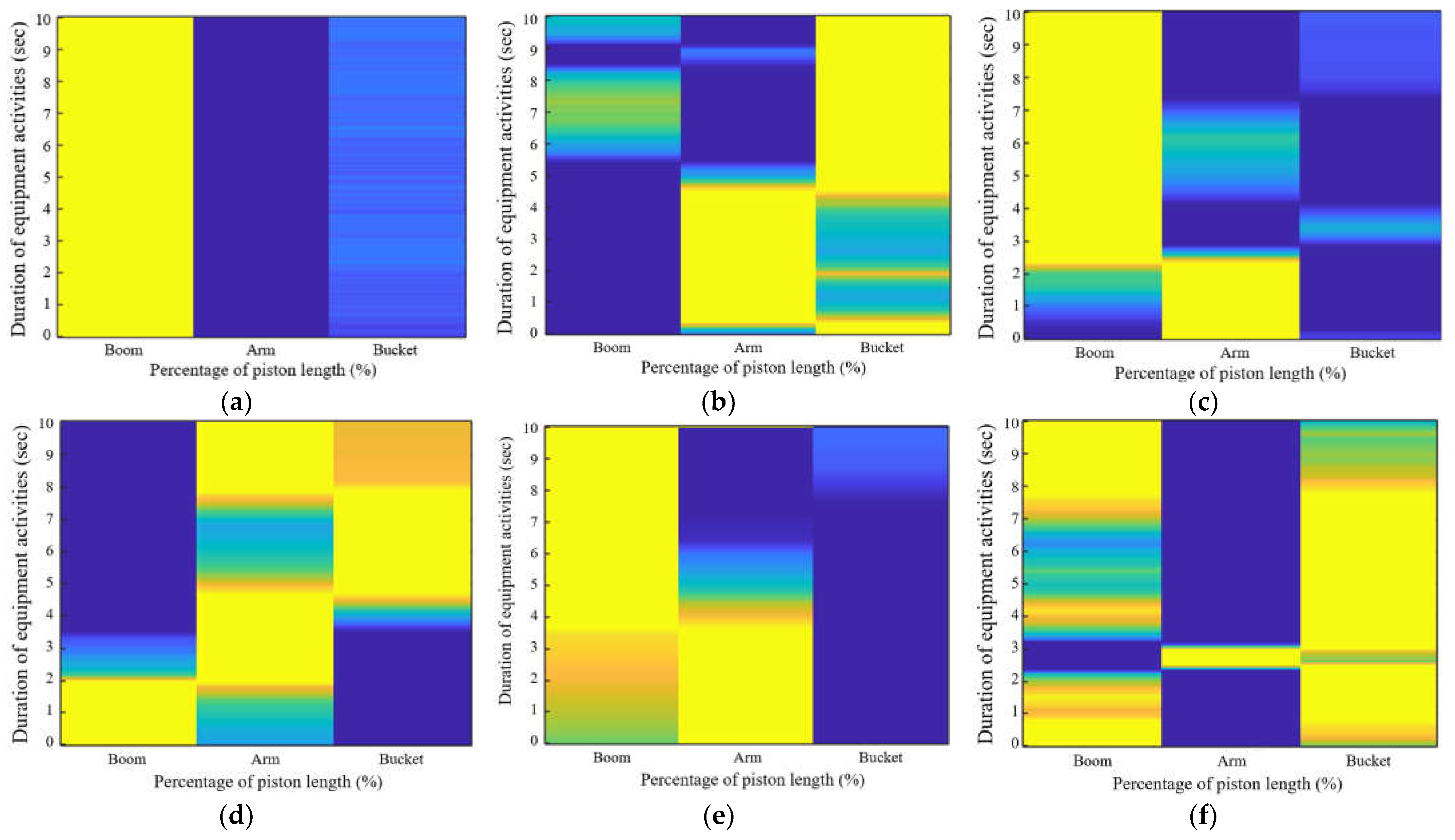
3.1. Equipment Activities for Analysis

From the excavator’s existing operations [6], we identified and defined six distinct areas to ascertain whether the activity identification ability of the developed DCNN could be based on piston displacement (movement) (

Table 1. Criteria for commencement and completion of activities (visual assessment).

No.	Activity	Description	Start	End	Image
1	Waiting	Standby state, without performing any operations	No movement	No movement
2	Scraping	Gathering or pushing surface soil with a constant height	No soil in the bucket, and the blade touches the ground	The bucket moves in the opposite direction after dragging
3	Excavating (under)	Digging below the ground to excavate soil	The blade touches the soil	The bucket is filled with soil and is fixed
4	Excavating (front)	Excavating soil from the surface at a specific location	The blade moves down to the ground	The blade comes up from the ground, and the boom is fixed
5	Dumping	Disposing of the collected soil from the bucket	The bucket piston contracts with soil in the bucket	The soil is emptied from the bucket, and the bucket piston is fixed
6	Repositioning	Adjusting its position by supporting the body with the boom on the ground	Place the bucket in a stable position on the ground	After the body is raised and lowered, lift the bucket

).

3.2. Data Collection and Participants

An excavator’s arm comprises three articulation points, each of which is equipped with a piston that contracts and expands. The arm moves to the maximum/minimum angle of each articulation point according to the length of the piston’s contraction and expansion. In other words, the displacement of the piston corresponds in a 1:1 ratio with the angle of the articulation point; thus, measuring the position of the articulation point and the maximum/minimum displacement of the piston from the equipment specifications or directly collected data allows us to evaluate the current movement of the excavator based solely on the piston’s motion. In this study, a distance sensor was installed for each piston of the three articulation points, which allowed us to measure the piston displacement of the boom, arm, and bucket, thereby capturing the equipment’s movements as relevant data.

The experiment was conducted using a scale model of an excavator (one-twelfth scale). The differences between the minimum and maximum displacement of the boom, arm, and bucket pistons were 13.2 cm, 15.3 cm, and 11.5 cm, respectively, and the measured ranges of the rotation angles were 97°, 110°, and 207°. Here, three sensors were mounted on a single Arduino Mega 2560 compatible board to measure the piston displacement of the three points, as shown in Figure 1.

The sensor used in this study was the VL53L0X-V2 equipped with the VL53L0X time of flight (ToF) module. This sensor is very small, and the distance detection function within a stable range—which was measured targeting a specific point in the experiment—exhibited a detectable distance range of 10 to 300 mm. The technical specifications of the VL53L0X-V2 ToF sensor are given in

Table 2. Technical specifications of VL53L0X-V2 ToF Sensor.

Feature	Details
Package	Optical LGA12
Size	4.40 × 2.40 × 1.00 mm
Operating voltage	2.6 to 3.5 V
Operating temperature	−20–70 °C
Infrared emitter	940 nm
I2C	Up to 400 kHz (FAST mode) serial bus Address: 0 × 52
Detectable distance	10–300 mm (experimental measurements)

. The meanings of each feature item are as follows: Package indicates the type of housing for the sensor module equipped with the ToF sensor; Size indicates the dimensions of the sensor module; Operating Voltages indicates the range of voltages required for the sensor to operate normally; Operating Temperature indicates the range of temperatures within which the sensor can function properly; I2C indicates the type of interface used for communication between the sensor and a microcontroller; Detectable Distance indicates the minimum and maximum distances that the sensor can detect; Infrared emitter indicates the wavelength of the infrared light-emitting diode used for distance detection.

The connection details of the sensors are shown in Figure 2. Each sensor was connected to the controller to acquire the respective distance values. The controller received the individual sensor values, which were stored based on predetermined waiting times. Here, the measurement time and distance values were recorded in a matrix and transmitted to the host computer. The data measurement interval was set to 20 frames per second. The model was trained in the MATLAB 23.2.0 (R2023b) environment, 64-bit Windows 11 system with the following hardware configuration: an NVIDIA GeForce GTX 1080GPU, 16 gigabytes, and Intel(R) Core (TM) i7-13650HX.

3.3. Detecting Equipment Activity

3.3.1. Aligning Data Standards

The experimental participants (five males aged 27–34 years) conducted 45 trials for each of the six movements. Here, the measurement time for each operation was set to 10 s.

The data configuration to measure the operational activities of the equipment is shown in Figure 3. Inside the dataset folder, there are subfolders for the equipment operational activity data measured by the five participants. Inside each subfolder, there are six datasets for each operational activity. Each dataset was measured at a rate of 20 frames per second, where 10 s of activity was considered as a single sample. Thus, data for 200 frames constitute one sample, and each activity accumulated 13,800 frames in one .m file (i.e., Matlab script file format) by acquiring 69 samples per activity. With 69 samples for each activity, for five individuals, a total of 2070 boom, arm, and bucket piston displacement samples were used.

Note that the minimum and maximum displacements of the pistons vary at each position; thus, the piston length data for each position was normalized to 0 and 1 by dividing by the length to conduct a uniform analysis as follows:

Pl_n[k] = (l_n[k])/(lM_n − lm_n)

Here, PL denotes the vector containing the normalized percentages of piston displacement, where n specifies the piston category (1 = boom; 2 = arm; and 3 = bucket). The index k represents the frame index within the dataset, l is the measured piston displacement, lM and lm are the maximum and minimum displacements observed for the piston, respectively.

3.3.2. Data Analysis Techniques

The converted length data of each piston based on a consistent percentage scale can be represented, as shown in Figure 4, where the vertical axis represents the elapsed time in frames recorded. As one sample is measured at 10 s intervals, the y-axis is limited to a minimum of 0–10 s. The x-axis is separated for the data measured from each piston, and it ranges from 0–1 based on the colors indicated on the right. Values closer to 1 indicate that the piston length reached its maximum, and values closer to 0 indicate the opposite.

Figure 4 shows the samples measured in a randomly steered state, thereby exhibiting the absence of a consistent pattern. The part marked in the red box shows the maximum values of the boom, arm, and bucket piston at 4.5 s of observation time, close to 1, 0.5, and 0, respectively. At this time, the excavator shows the boom as high as possible, the arm bent inward, and the bucket bent inward as much as possible.

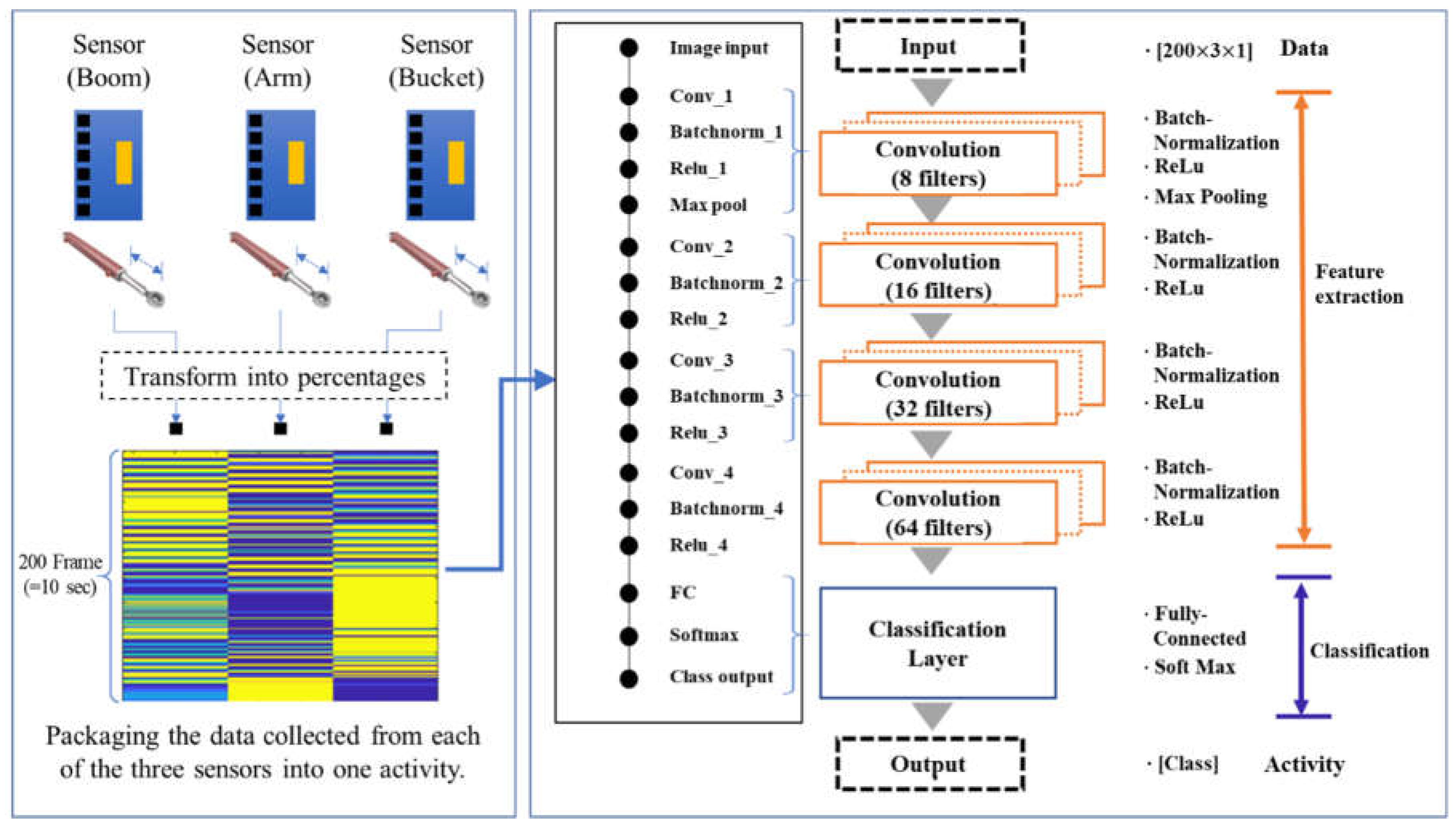
3.3.3. DCNN-Based Activity Recognitions

In this study, a DCNN-based classifier was implemented to train the activity data of the classified equipment (Figure 5). The proposed DCNN model was designed to process a set of data provided by three pistons, equivalent to 10 s of activity (or 200 frames). It aims to analyze complex signal data (as though examining a single image) by extracting significant features from the dataset. In order to achieve this, the model was developed by the author without employing the backbone net architectures such as ResNet, MobileNet, or ShuffleNet.

In Figure 5, the distance values measured by each ToF sensor module are normalized to a value between 0 and 1 and are captured in a frame. An activity set comprises 200 such frames. The proposed DCNN model architecture consists of four main components (an input section, a feature extraction stage, a classification stage, and an output section).

• Input section

For this study, a 200 × 3 matrix was input, and a total of 2070 samples were used. It consists of five participants, six activities for each individual, and 69 samples for each activity.

• Feature extraction stage

The feature extraction stage is composed of a convolutional block that varies from one to four steps. In our DCNN architecture, the feature extraction module comprises four sequentially arranged convolution blocks. Each block is strategically designed to enhance the network’s ability to discern increasingly complex patterns within the input data. The configuration of these blocks is as follows:

Convolution Block 1: This initiates the feature extraction process with a convolution-2D layer employing 3 × 3 kernels and eight filters, incorporating the “Padding” of 1 pixel to maintain spatial dimensions. This is followed by a batch-normalization layer to normalize the activations and facilitate stable learning. The Relu layer introduces nonlinearity, allowing for the representation of complex functions. The block concludes with a max-pooling-2D layer (2 × 2; stride = 1) to reduce feature map dimensions while preserving the most salient features.

Convolution Block 2: This utilizes a convolution-2D layer with 3 × 3 kernels, increasing the filter count to 16, to capture a wider array of features. A subsequent batch-normalization layer ensures the consistency of activations. The inclusion of a Relu layer maintains the network’s capacity for nonlinear feature representation.

Convolution Block 3: This further augments the network’s feature detection capabilities with another Convolution-2D layer, with 32 filters this time. A batch-normalization layer follows for activation normalization. A Relu layer is used, again, to apply nonlinearity to the feature maps.

Convolution Block 4: The final convolution block scales up the complexity with a Convolution-2D layer that utilizes 64 filters, enabling the network to capture the most abstract features. This is paired with a batch-normalization layer for maintaining activation consistency across batches. The block is completed with a Relu layer for nonlinear activation, which is crucial for complex pattern recognition.

• Classification stage

The classification stage directly addresses the task of assigning class probabilities to the input samples. The stage is structured as follows:

Fully connected layer: The classification stage initiates with a fully connected layer comprising six neurons, each representing one of the potential class outcomes. This layer acts as a bridge, synthesizing the high-level features extracted by the preceding convolutional blocks into a format suitable for classification. The number of neurons in this layer corresponds to the total number of classes within the dataset, allowing for a dense representation of the learned features.

Softmax layer: Subsequent to the fully connected layer, a Softmax layer is employed to convert the raw class scores emanating from the fully connected layer into probabilities. The Softmax function ensures that the output scores are normalized, resulting in a probability distribution over the class labels. This step is critical for multi-class classification tasks, as it provides a clear probabilistic interpretation of the model’s predictions.

Classification layer: The final component of the classification stage is the classification layer, which serves to quantify the discrepancy between the predicted class probabilities and the true class labels. This layer computes the loss during the training process, facilitating the optimization of the network’s parameters. By minimizing this loss, the model learns to improve its predictions, enhancing its ability to accurately classify incoming samples.

• Output section

The output section serves as the definitive assessment of the network’s classification capabilities. It not only provides a clear indication of the predicted class for each input but also offers a probabilistic insight into the model’s confidence regarding its predictions. In this study, the network is tasked with the classification of six distinct activities: Waiting, Scraping, Excavating (under), Excavating (front), Dumping, and Repositioning.

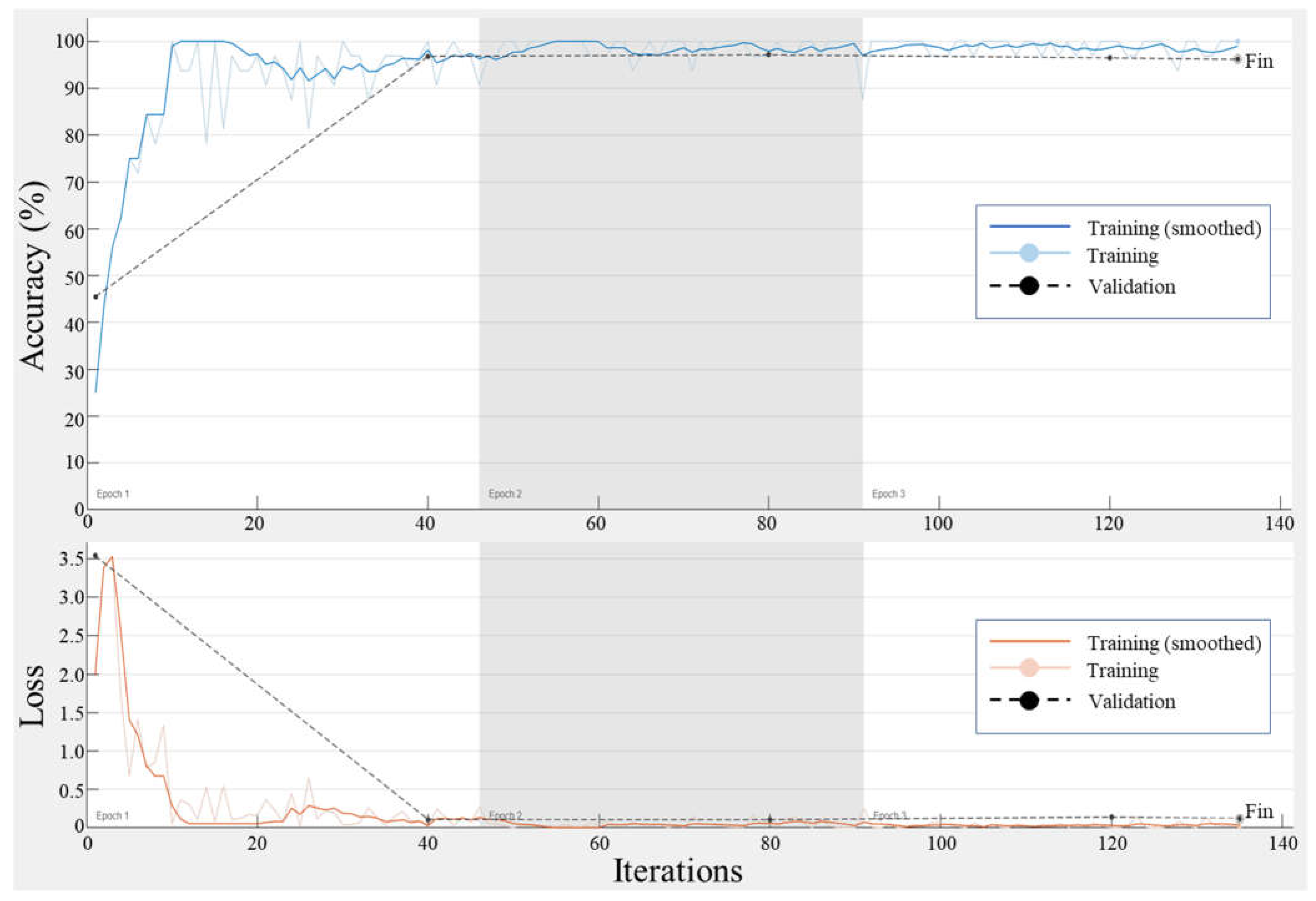
• Training options configuration

The classification stage directly addresses the task of assigning class probabilities to the input samples. The model training was conducted in the MATLAB environment, using the Deep Learning Toolbox. For the training process, we selected the Adam optimization algorithm for its effectiveness with complex datasets. The parameters defined through the training options are shown in

Table 3. Hyperparameter configuration for model training.

Parameter	Value	Description
Gradient Decay Factor	0.9	Rate at which past gradients are decayed.
Squared Gradient Decay Factor	0.999	Rate at which past squared gradients are decayed.
Epsilon	1 × 10−8	Constant added to prevent division by zero.
Initial Learning Rate	1 × 10−3	Starting learning rate for the training process.
Max Epochs	3	Maximum number of epochs for training.
Learning Rate Schedule	‘none’	Approach to adjusting the learning rate (constant in this study).
Learning Rate Drop Factor	0.1	Factor by which the learning rate is reduced when scheduled.
Learning Rate Drop Period	10	Epochs between learning rate reductions.
Mini-Batch Size	32	Number of samples per gradient update.
Shuffle	‘once’	Shuffling of the dataset before training.
L2 Regularization	1 × 10−4	Regularization factor to prevent overfitting.
Gradient Threshold Method	‘L2Norm’	Method for clipping gradients (not applied with ‘Inf’ threshold).
Gradient Threshold	Inf	Threshold for gradient clipping.

.

4. Results and Discussion

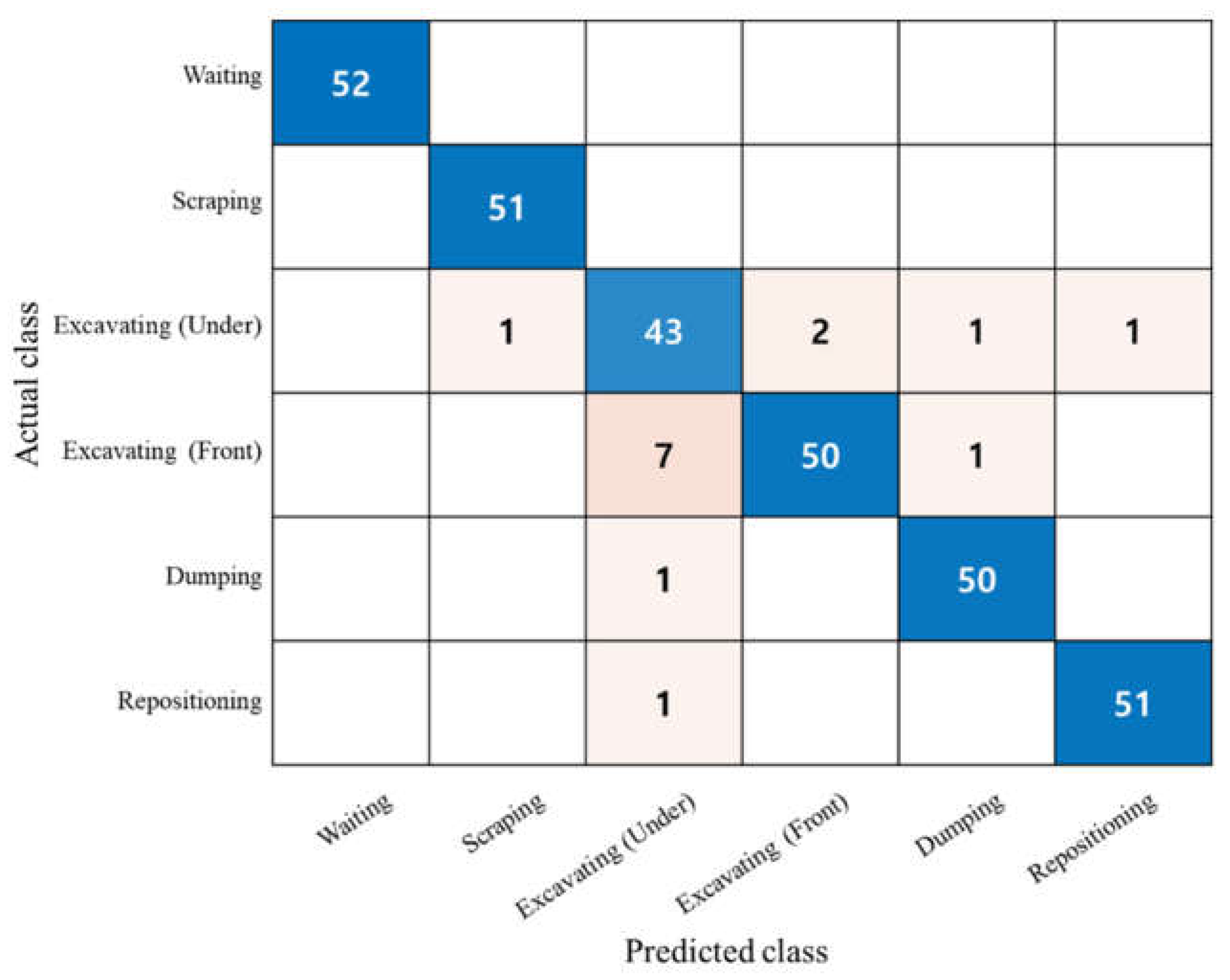
4.1. Performance Verification of the Proposed Model

One sample comprises 200 sets of piston displacement ratio values, recorded as time series data over a 10-s period. Figure 6 shows the sample data matrices for each activity used in the classifier. As can be seen, the patterns of the six activities are visually distinguishable, and this clarity is reflected in the confusion matrix of the data classifier.

The color pattern during the waiting state shows little change, but it is presumed that frequent color changes occur in the data from the bucket due to vibrations causing shaking (Figure 6a).

Scraping is the action of pushing or collecting soil on the ground while maintaining a constant height. In Figure 6b, the fact that the overall color of the boom pattern is close to blue means that the excavator is moving while maintaining the boom in a lowered state close to the ground. In the bucket pattern, the movement changed frequently enough to change to orange three times, which means that when the arm is not moving, scraping is performed by manipulating the bucket.

Excavating (under) and Excavating (front) both achieve the same result of putting soil into the bucket, but a clear difference can be seen through pattern analysis (Figure 6c,d). In the case of ‘Under’, the color of the boom pattern shifts from blue to yellow, signifying the action of significantly lifting the boom as it nears the completion of the activity. Conversely, in the case of ‘Front’, the color transitions from yellow to blue, denoting that the boom is undergoing a folding motion. The number of color changes and the intervals between them in the actions of the arm and the bucket demonstrate similar patterns. This similarity is analyzed to be due to the identical process of digging soil into the bucket and lifting it to prevent soil loss. In the ‘under’ scenario, beyond the initial phase (approximately 0 to 2.5 s), a piston length ratio of less than 50% for the arm and bucket was observed in most frames. However, in the ‘front’ scenario, a piston length ratio of more than 50% was observed in most frames. This difference occurs because the action taken to prevent soil loss from the bucket is consistent, yet the rotation angles of the arm and bucket that effectively prevent soil loss vary depending on the boom’s position. As a result, although behaviorally similar patterns (sections of color change) are observed in both cases, it can be concluded that the actual actions differ significantly according to the pattern.

Dumping refers to the process of transferring soil from a bucket to a specified location. In Figure 6e, the boom is raised for the initial 3.5 s. Subsequently, for about 7 s, the activity concludes with the bucket being adjusted by the arm to ensure it is moved to the correct position.

Repositioning involves adjusting the main body’s position for optimal excavation. In Figure 6f, the color change frequency of the boom pattern was primarily observed. The main change in arm pattern occurred in two vectors, beginning from 2 to 3 s.

A total of 2070 samples were used as training data for the model. Consequently, the 2070 samples utilized for verification correspond to 5.75 h when converted into video time, or 414,000 frames when converted into image count.

In the training process, 1758 samples (75% of the 2070 samples) were used as the training set. In Figure 7, the rate of change in precision and loss rate decreased significantly at 40 iterations, and learning ended at 135 iterations. The verification accuracy was measured at 96.15%.

In the validation process, 312 samples (15% of the 2070 samples) were used as the validation set. Figure 8 shows the performance of the classifier using a confusion matrix. In this study, there were six classes, and the confusion matrix was expressed as a 6 × 6 matrix. The diagonal values of the confusion matrix represent correctly classified predictions (True Positives, TP). Off-diagonal rows of the target class represent predictions that were misclassified as other classes (False Positives, FP). Off-diagonal columns of the target class represent predictions that were incorrectly classified into that class (False Negatives, FN).

In the model, precision refers to the cases where the observed class is indeed the corresponding class, while recall is an indicator of whether the actual target has been predicted as the respective class. The precision for each observation can be expressed as TP/(TP + FP), and recall can be expressed as TP/(TP + FN). For instance, when considering the class ‘Excavating (Under),’ precision is calculated as 43/(43 + 7 + 1 + 1), resulting in a value of 0.8269, while recall is calculated as 43/(1 + 43 + 2 + 1 + 1), resulting in a value of 0.8958.

The precision for each class, from waiting to repositioning, is sequentially listed as 100%, 100%, 82.69%, 96.15%, 96.15%, and 98.08%, with an average precision of 95.51%. The recall for each class is sequentially listed as 100%, 100%, 89.58%, 86.21%, 98.04%, and 98.08%, with an average recall of 95.31%.

Accuracy is an indicator of predictive correctness across all cases relative to all classes, and it can be represented as (the sum of True Positives (TP) + the sum of True Negatives (TN))/total number of cases. In the proposed model, the accuracy of the model is calculated as (52 + 51 + 43 + 50 + 50 + 51)/312 = 0.9519, i.e., 95.19%.

4.2. Comparison with Other Models

In this study, the results are compared with the activity classification models in recent research (

Table 4. Performance metrics comparison.

No.	Method	Category	Data Set	Activity	Performance Metrics
					Precision	Recall	Accuracy
1	C. Chen, et al. [7]	Vision (Image size: 1280 × 720)	351	Digging	95	86
				Swinging	86	93
				Loading	84	80
				Average	88	88	87.6
2	Slaton T, et al. [12]	Sensor (Acceleration sensor)	242	Idling	100	81
				Traveling	99	57
				Scooping	73	96
				Dropping	83	65
				Rotating (left)	69	93
				Rotating (right)	94	80
				Average	85	83	83
3	Proposed Model	Sensor (Distance sensor)	312	Waiting	100	100
				Scraping	100	100
				Excavating (Under)	82.7	89.6
				Excavating (Front)	96.2	86.2
				Dumping	96.2	98.0
				Repositioning	98.1	98.1
				Average	95.5	95.3	95.2

). The comparative analysis has consolidated the findings from studies based on image data and sensor-based research in comparison with the proposed model.

The data used for verification in the vision-based model [7] consisted of 351 video clips with a resolution of 1280 × 720 pixels, and these were collected from 21 different construction sites, considering the site conditions, equipment viewpoints, and scales and colors of the excavators. The sensor-based model [12] utilized two three-axis accelerometers, one near the bucket and one on the excavator body, to collect six data points as a single vector. A total of 48,435 vectors were used for training. A vector recorded over two s at a rate of 100 Hz was treated as a single sample, and the number of such samples used in training was considered to be 242.

In terms of accuracy, recall, and accuracy, the first model (vision model) and the second model (acceleration sensor model) showed higher measurements for the first model. On the other hand, the distance sensor model (proposed model) demonstrated superior performance, with all metrics exceeding 95%, compared to the other two models. In the comparison of individual activities, the vision model demonstrated a high precision rate at 95% in Digging and a high recall rate at 93% in Swinging. However, it exhibited lower performance in Loading, with a precision rate of 88% and a recall rate of 80%. The acceleration sensor model displayed high precision rates of 100%, 99%, and 94% in Idling, Traveling, and Rotating (right), respectively. However, it showed lower metrics in Traveling and Dropping, with precision rates of 57% and 65%, respectively. On the other hand, the distance sensor model shows a rate of precision and recall of above 90% in most metrics, excluding excavating. As can be seen in Figure 8, even the errors that indicate lower metrics are due to discrepancies between the ‘Under’ and ‘Front’ cases. It is expected that integrating these two metrics for experimentation as an activity would result in a lower error rate.

In the comparison of average accuracy, the vision model exhibits a result of 87.6%, the acceleration sensor model shows 83%, and the distance sensor model demonstrates 95.2%. It is speculated that one reason for the better performance of models 1 and 3 compared to model 2 could be the larger amount of validation data sets for the first and third models.

Based on the comparison of the three models, the following conclusion can be drawn: when an equivalent level of datasets is available, the proposed model was able to achieve a higher average accuracy than the vision-based detection models. In comparison with non-vision-based models, the distance sensor-based model consistently demonstrated improved performance in precision and recall for each class over the acceleration sensor-based model.

4.3. Contributions and Limitations

In this study, a new methodology based on a DCNN for detecting construction equipment activity using sensor data, as well as a data collection approach, is presented.

We reveal a DCNN (deep convolutional neural network) methodology capable of detecting construction equipment activity information, including time series data, by utilizing distance sensors to store the displacement of three pistons as a single vector and treating the 200 accumulated vectors as one activity sample. In the experiments conducted on the one-twelfth scale model, this methodology demonstrated a higher level of accuracy compared to image-based and accelerometer-based methodologies. In the vision-based study [7], it was explained that detection errors in the sample cases occurred due to variations in the vision-based model’s training data (video), such as shadows, the position of the observation camera, the posture of the subject under observation, and the lighting conditions at the time of recording. In the accelerometer-based study [35], it is mentioned that numerous experiments are required to obtain additional training data, making data expansion challenging and necessitating a large volume of data. This issue may arise due to significant variances in the values measured by the accelerometer, which can vary according to the excavator’s size and shape, work speed, and the placement of the accelerometer. Therefore, it is expected that securing a diverse range of additional data is necessary.

On the other hand, in the proposed method, data acquisition is facilitated by using a time of flight (ToF) distance sensor module. This module measures the distance by calculating the time it takes for light emitted at a specific frequency to bounce back from the target. Furthermore, the patterns learned from a specific excavator, based on the piston length ratio, can be applied to excavators with different specifications. If the current piston length ratio can be determined, the developed data collection method and learning model can be directly applied without modification. This advantage can overcome the problem that vision-based models face, which is the need to separately train excavators of different forms (such as color and size). Since the collected data represent solely the activity of the excavator, this fundamentally solves the issue of accuracy degradation caused by noise (all pixels, excluding the observed object) that is included in a single vector along with the observation subject in vision-based research.

Accelerometer data, which estimate excavator movements through changes in speed, makes reproducing the original actions difficult. It is speculated that this data loss during the pattern estimation process contributes to discrepancies in precision and recall among the classes (refer to Table 4). Conversely, in the proposed methodology, by accurately preserving the core movement data of the equipment, including the piston displacement of each part over time, a perfect reproduction of the collected data is achieved. This approach is analyzed to result in higher performance compared to other methods.

The limitations of this study are as follows. This research relies on limited data obtained from three pistons, excluding information such as the rotation of the excavator body, the movement of the undercarriage, and the amount of soil in the bucket. However, even with just the movement of three pistons, the performance in a constrained experimental environment has been shown to be commendable. This issue can be addressed by installing additional sensors to increase the data volume for each vector and by expanding the model’s input data format. Moreover, the experiments were conducted using a one-twelfth scale model without the participation of professional excavator operators. Therefore, future research should involve real excavators and experts to compare the differences between the scale and actual experiments and to verify the practical applicability of the data.

4.4. Generalizability of the Proposed Method

Conventional methods involve essential elements, e.g., camera equipment and shooting angles, the observer’s labor cost, and the analyst’s labor cost, and such methods have economic and temporal limitations relative to securing large amounts of data. In contrast, the proposed method, including the sensors and analysis model, can be employed to record and analyze the duration of each task for all on-site equipment when equipped with sensors that can measure the piston displacement of real-world equipment using data loggers. Compared with vision-based methods, the proposed method allows for long-term data collection because the capacity of data storage space is greatly reduced. Compared to a vision-based detection model that uses an image of size 1280 × 720 pixels as its basic input data, the model requires storage space for three primary colors (e.g., red, green, blue) for each of the 1280 × 720 pixels. Therefore, a total of 2,764,800 pieces of color information are needed. However, in this study, only three pieces of piston length information are needed for the analysis of the same vector. In this study, the training data consist of 69 samples (200 vectors per sample) from six actions performed by five individuals, with a total of 414,000 vectors and a total data volume of only 2.24 megabytes. Assuming that an image of 1280 × 720 pixels containing 2,764,800 pieces of data requires 1 byte per piece, each vector would require 2.64 MB of storage space. In order to store data for learning in an experiment under the same conditions, 1,092,960 megabytes (about 1067 gigabytes or 1.04 terabytes) of storage space is required. Thus, it can be used to obtain a large amount of relevant and quantitative data over time at the same investment cost.

Furthermore, the proposed method can be set up as an independent historical observation device, offering advantages in practical applications that encounter observation blind spots or disruptions in satellite communication. It is particularly beneficial in scenarios such as tunnel and underground construction, nighttime operations, or conditions where distinguishing object boundaries becomes challenging due to extremely bright or dim lighting.

5. Conclusions

In this study, we successfully developed a non-visual method for detecting construction equipment activities using time of flight (ToF) distance sensors and a deep convolutional neural network (DCNN). Our method showcased superior performance in accuracy, precision, and recall compared to traditional approaches, demonstrating its potential for real-world construction site monitoring. However, future research is needed to validate these findings in larger, real-world settings and to explore the integration of additional sensor data for enhanced accuracy.

References

1. Cheng, C.-F.; Rashidi, A.; Davenport, M.A.; Anderson, D.V. Activity Analysis of Construction Equipment Using Audio Signals and Support Vector Machines. Autom. Constr. 2017, 81, 240–253. [Google Scholar] [CrossRef]
2. Harichandran, A.; Raphael, B.; Mukherjee, A. A Hierarchical Machine Learning Framework for the Identification of Automated Construction. J. Inf. Technol. Constr. 2021, 26, 591–623. [Google Scholar] [CrossRef]
3. Yang, J.; Park, M.-W.; Vela, P.A.; Golparvar-Fard, M. Construction Performance Monitoring via Still Images, Time-Lapse Photos, and Video Streams: Now, Tomorrow, and the Future. Adv. Eng. Inform. 2015, 29, 211–224. [Google Scholar] [CrossRef]
4. Lu, M.; Dai, F.; Chen, W. Real-Time Decision Support for Planning Concrete Plant Operations Enabled by Integrating Vehicle Tracking Technology, Simulation, and Optimization Algorithms. Can. J. Civ. Eng. 2007, 34, 912–922. [Google Scholar] [CrossRef]
5. Akhavian, R.; Behzadan, A.H. Construction Equipment Activity Recognition for Simulation Input Modeling Using Mobile Sensors and Machine Learning Classifiers. Adv. Eng. Inform. 2015, 29, 867–877. [Google Scholar] [CrossRef]
6. Peurifoy, R.L.; Schexnayder, C.; Schmitt, R.; Shapira, A. Construction Planning, Equipment, and Methods, 9th ed.; McGraw-Hill Education: New York, NY, USA, 2018. [Google Scholar]
7. Chen, C.; Zhu, Z.; Hammad, A. Automated Excavators Activity Recognition and Productivity Analysis from Construction Site Surveillance Videos. Autom. Constr. 2020, 110, 103045. [Google Scholar] [CrossRef]
8. Duan, R.; Deng, H.; Tian, M.; Deng, Y.; Lin, J. SODA: A Large-Scale Open Site Object Detection Dataset for Deep Learning in Construction. Autom. Constr. 2022, 142, 104499. [Google Scholar] [CrossRef]
9. Xiao, B.; Kang, S.-C. Development of an Image Data Set of Construction Machines for Deep Learning Object Detection. J. Comput. Civ. Eng. 2021, 35, 05020005. [Google Scholar] [CrossRef]
10. Lee, Y.-C.; Scarpiniti, M.; Uncini, A. Advanced Sound Classifiers and Performance Analyses for Accurate Audio-Based Construction Project Monitoring. J. Comput. Civ. Eng. 2020, 34, 04020030. [Google Scholar] [CrossRef]
11. Jung, S.; Jeoung, J.; Lee, D.; Jang, H.; Hong, T. Visual–Auditory Learning Network for Construction Equipment Action Detection. Comput.-Aided Civ. Infrastruct. Eng. 2023, 38, 1916–1934. [Google Scholar] [CrossRef]
12. Slaton, T.; Hernandez, C.; Akhavian, R. Construction Activity Recognition with Convolutional Recurrent Networks. Autom. Constr. 2020, 113, 103138. [Google Scholar] [CrossRef]
13. Rashid, K.M.; Louis, J. Automated Activity Identification for Construction Equipment Using Motion Data from Articulated Members. Front. Built Environ. 2020, 5, 144. [Google Scholar] [CrossRef]
14. Langroodi, A.K.; Vahdatikhaki, F.; Doree, A. Activity Recognition of Construction Equipment Using Fractional Random Forest. Autom. Constr. 2021, 122, 103465. [Google Scholar] [CrossRef]
15. Montaser, A.; Moselhi, O. RFID+ for Tracking Earthmoving Operations. In Proceedings of the Construction Research Congress 2012, West Lafayette, IN, USA, 21–23 May 2012; American Society of Civil Engineers: Reston, VA, USA, 2012; pp. 1011–1020. [Google Scholar]
16. Golparvar-Fard, M.; Heydarian, A.; Niebles, J.C. Vision-Based Action Recognition of Earthmoving Equipment Using Spatio-Temporal Features and Support Vector Machine Classifiers. Adv. Eng. Inform. 2013, 27, 652–663. [Google Scholar] [CrossRef]
17. Memarzadeh, M.; Golparvar-Fard, M.; Niebles, J.C. Automated 2D Detection of Construction Equipment and Workers from Site Video Streams Using Histograms of Oriented Gradients and Colors. Autom. Constr. 2013, 32, 24–37. [Google Scholar] [CrossRef]
18. Xiao, B.; Kang, S.-C. Vision-Based Method Integrating Deep Learning Detection for Tracking Multiple Construction Machines. J. Comput. Civ. Eng. 2021, 35, 04020071. [Google Scholar] [CrossRef]
19. Kim, J.; Chi, S. Action Recognition of Earthmoving Excavators Based on Sequential Pattern Analysis of Visual Features and Operation Cycles. Autom. Constr. 2019, 104, 255–264. [Google Scholar] [CrossRef]
20. Shen, Y.; Wang, J.; Feng, C.; Wang, Q. Dual Attention-Based Deep Learning for Construction Equipment Activity Recognition Considering Transition Activities and Imbalanced Dataset. Autom. Constr. 2024, 160, 105300. [Google Scholar] [CrossRef]
21. Bohn, J.S.; Teizer, J. Benefits and Barriers of Construction Project Monitoring Using High-Resolution Automated Cameras. J. Constr. Eng. Manag. 2010, 136, 632–640. [Google Scholar] [CrossRef]
22. Zhang, S.; Zhang, L. Vision-Based Excavator Activity Analysis and Safety Monitoring System. In Proceedings of the 38th International Symposium on Automation and Robotics in Construction, Dubai, United Arab Emirates, 2–4 November 2021. [Google Scholar]
23. Zhang, J.; Zi, L.; Hou, Y.; Wang, M.; Jiang, W.; Deng, D. A Deep Learning-Based Approach to Enable Action Recognition for Construction Equipment. Adv. Civ. Eng. 2020, 2020, 8812928. [Google Scholar] [CrossRef]
24. Cheng, T.; Venugopal, M.; Teizer, J.; Vela, P.A. Performance Evaluation of Ultra Wideband Technology for Construction Resource Location Tracking in Harsh Environments. Autom. Constr. 2011, 20, 1173–1184. [Google Scholar] [CrossRef]
25. Teizer, J.; Venugopal, M.; Walia, A. Ultrawideband for Automated Real-Time Three-Dimensional Location Sensing for Workforce, Equipment, and Material Positioning and Tracking. Transp. Res. Rec. J. Transp. Res. Board. 2008, 2081, 56–64. [Google Scholar] [CrossRef]
26. Shahi, A.; Aryan, A.; West, J.S.; Haas, C.T.; Haas, R.C.G. Deterioration of UWB Positioning during Construction. Autom. Constr. 2012, 24, 72–80. [Google Scholar] [CrossRef]
27. Montaser, A.; Bakry, I.; Alshibani, A.; Moselhi, O. Estimating Productivity of Earthmoving Operations Using Spatial Technologies 1 This Paper Is One of a Selection of Papers in This Special Issue on Construction Engineering and Management. Can. J. Civ. Eng. 2012, 39, 1072–1082. [Google Scholar] [CrossRef]
28. Vahdatikhaki, F.; Hammad, A. Framework for near Real-Time Simulation of Earthmoving Projects Using Location Tracking Technologies. Autom. Constr. 2014, 42, 50–67. [Google Scholar] [CrossRef]
29. Mathur, N.; Aria, S.S.; Adams, T.; Ahn, C.R.; Lee, S. Automated Cycle Time Measurement and Analysis of Excavator’s Loading Operation Using Smart Phone-Embedded IMU Sensors. In Proceedings of the Computing in Civil Engineering 2015, Austin, TX, USA, 21–23 June 2015; American Society of Civil Engineers: Reston, VA, USA, 2015; pp. 215–222. [Google Scholar]
30. Akhavian, R.; Behzadan, A.H. An Integrated Data Collection and Analysis Framework for Remote Monitoring and Planning of Construction Operations. Adv. Eng. Inform. 2012, 26, 749–761. [Google Scholar] [CrossRef]
31. Ahn, C.R.; Lee, S.; Peña-Mora, F. Application of Low-Cost Accelerometers for Measuring the Operational Efficiency of a Construction Equipment Fleet. J. Comput. Civ. Eng. 2015, 29, 04014042. [Google Scholar] [CrossRef]
32. Bae, J.; Kim, K.; Hong, D. Automatic Identification of Excavator Activities Using Joystick Signals. Int. J. Precis. Eng. Manuf. 2019, 20, 2101–2107. [Google Scholar] [CrossRef]
33. Rashid, K.M.; Louis, J. Times-Series Data Augmentation and Deep Learning for Construction Equipment Activity Recognition. Adv. Eng. Inform. 2019, 42, 100944. [Google Scholar] [CrossRef]
34. Kingma, D.P.; Ba, J. Adam: A Method for Stochastic Optimization. arXiv 2014, arXiv:1412.6980. [Google Scholar]
35. Kim, J.; Chi, S.; Ahn, C.R. Hybrid Kinematic–Visual Sensing Approach for Activity Recognition of Construction Equipment. J. Build. Eng. 2021, 44, 102709. [Google Scholar] [CrossRef]
Figure 1. Installed sensors and boards: (a) One-twelfth scale model and sensor system configuration; (b) ToF sensor and reflector; (c) hydraulic piston installation.
Applsci 14 02859 g001
Figure 2. Connectivity diagram of ToF sensor.
Applsci 14 02859 g002
Figure 3. Piston length dataset structure.
Applsci 14 02859 g003
Figure 4. Data matrices for the percentage of each piston length.
Applsci 14 02859 g004
Figure 5. Example of the DCNN-based classifier for equipment activity data.
Applsci 14 02859 g005
Figure 6. Sample data matrices of each of the six activities: (a) Waiting; (b) Scraping; (c) Excavating (under); (d) Excavating (front); (e) Dumping; (f) Repositioning.
Applsci 14 02859 g006
Figure 7. Accuracy and loss across training iterations.
Applsci 14 02859 g007
Figure 8. Classification performance confusion matrix.
Applsci 14 02859 g008