Survivability Prediction of Open Source Software with Polynomial Regression

Abstract

In modern software development, OSS (Open Source Software) has become a crucial element. However, if OSS have few contributors and are lacking in maintenance activities, such as bug fixes, are used, it can lead to significant costs and resource allocation due to maintenance discontinuation. Since OSS are developed by a diverse group of contributors, the consistency of their involvement may vary, making continuous support and maintenance unpredictable. Therefore, it is necessary to identify the status of each OSS to avoid increased maintenance costs when selecting OSS for use. To address these issues, we use polynomial regression to predict trends in bug-fixing activities and evaluate the survivability of OSS accordingly. We predict the trend of bug-fixing activities in OSS, using factors such as popularity, number of contributors, and code complexity. A lower trend value indicates more vigorous activity. In this paper, we conduct data collection and extraction, generating model, and model testing and evaluation to predict survivability using these data. After collecting data through various tools, the models of different degrees are generated using K-fold cross-validation. The model with the highest performance is selected based on the RMSE (Root Mean Squared Error) and RSE (Residual Standard Error). Then, the chosen model is employed to predict the survivability of OSS and compare it with actual outcomes. This method is experimented with on OSS used in the KakaoTalk commercial messenger app. As a result, several OSS are predicted to have low survivability, and among them, five are analyzed. It is observed that, in reality, activities such as delayed or discontinued release updates occurred. These findings can support OSS users in selecting OSS for cost-saving purposes and alert OSS administrators to the need for solutions to ensure project survival.

1. Introduction

OSS (Open Source Software) has become a crucial part of modern software development, being applied in various fields, ranging from simple tools to complex operating systems [1]. While the adoption of OSS has greatly enhanced development convenience, it has also introduced various risks, such as project dependency issues [2]. The project dependency mainly refers to the possibility of the main project encountering issues due to bugs in open source components. These risks primarily arise from the collaborative nature of OSS development, where individuals and groups with diverse backgrounds participate autonomously, rather than being tied to a single organization. This characteristic may not guarantee the ongoing involvement of OSS contributors, which can impact its maintenance [3]. Decreased contributions can hinder bug-fixing efforts, leading to increased maintenance costs and efforts [4]. In fact, there have been cases where issues in OSS, such as the Shellshock incident [5], which affected several commercial software products, or changes in DNS resolver code in the GNUC library, resulted in the disruption of some applications when making network requests [6].

To mitigate these risks, it is important to utilize OSS that is maintained in the long term, ensuring high survivability into the future, and preemptively replace OSS that does not meet this criterion [7]. However, evaluating survivability criteria is not always clear, making it difficult for users to assess and take action. Therefore, it is necessary to evaluate the maintainability of OSS based on factors such as repository characteristics and current status and make informed choices. Previous studies have attempted to estimate OSS survivability by predicting the repository activity or estimating decreases in contributor numbers [8,9,10]. However, these studies focused on overall development activities, including project dependencies, which limited their ability to accurately assess the remaining risks related to bugs.

In this paper, we propose predicting the survivability of OSS using polynomial regression. We predict the trend of bug-fixing activities based on popularity, the number of contributors, and the code complexity of OSS. A higher value indicates a lower likelihood of survival. To address this, we formulated the two following RQs (research questions):

RQ1

Can the survivability of OSS be predicted through polynomial regression?

RQ2

Can the survivability of OSS be modeled through polynomial regression?

RQ1 concerns the ability of polynomial regression to accurately reflect the survivability of OSS based on the predicted target. RQ2 explores the feasibility of using polynomial regression to predict the target with the given features. To achieve this, we conduct three main steps: data collection and extraction, regression model setup and testing, and evaluation. Firstly, we collect information such as star counts and code complexity from project repositories using GitHub API and static analysis tools, and then the extract trend of OSS values representing the bug-fixing activity from the collected data. In the second step, we perform K-fold cross-validation for various degree values and select the degree showing the best performance to create the model. In the final step, we predict the survivability of OSS using the generated model. To demonstrate the model’s performance, we compare the predicted results with the current state and features of the actual OSS. Additionally, the accuracy and fitness of the model are verified using RMSE (Root Mean Squared Error) and RSE (Residual Standard Error). These two metrics are employed to validate whether the model has been adequately trained and to ascertain the accuracy of the predictions made by the trained model. We conduct experiments targeting the OSS used in KakaoTalk commercial messenger app to validate our proposed method. We select these OSS components for evaluation to assess their viability in actual commercial applications. The results of the experiment predicted that numerous OSS projects would have a decreased likelihood of survival. Upon analyzing five of these projects, it was observed that all experienced a decline in various activities within the project repositories, such as delayed or discontinued updates to release versions. Therefore, we believe that using OSS predicted to have high survivability can help reduce maintenance costs. Based on these results, we anticipate that our research will contribute to preparing OSS users and potential users for the discontinuation of OSS maintenance, thereby reducing maintenance costs. Additionally, we believe that it can provide notifications to OSS administrators who wish for their projects to continue, enabling them to prepare various remedies for project operation in advance.

The remaining sections of this paper are structured as follows: Section 2 provides the necessary background knowledge, while Section 3 presents the proposed method for predicting OSS survivability. Section 4 describes the results of the experiments conducted on the proposed method. Finally, Section 5 concludes the paper and suggests future research directions.

2. Background

2.1. Survivability Prediction

The survivability of OSS, also known as sustainability, refers to whether an OSS will continue to exist in the future or fail [11]. We define indicators of survival and failure based on the level of activity in development and maintenance. Our research aims to predict the survivability to prevent increased costs due to maintenance stopping for open source users. Therefore, from the user’s perspective, survivability means continued development and maintenance in the future, including addressing new bug fixes and supporting the latest programming language versions. As such, we set the criterion for survivability based on the maintenance of OSS.

Software maintainability refers to the ease with which software can be modified, updated, and repaired over time [12]. Maintainability is an important factor in the long-term success of a software system. If maintainability is low, it becomes difficult to ensure that the system will continue to meet user requirements over time. Therefore, to maintain the quality of the software, high maintainability must be ensured. However, maintainability can be affected by the following factors:

• Project dependency: Software development projects can have dependencies on other systems or components. These dependencies can cause maintenance to be more difficult if failures in other systems affect the main system.
• Change management: Changes to software or dependencies must be managed to ensure that new issues do not arise. This is necessary to minimize the impact of changes on the system.
• Documentation: Documentation can provide a clear understanding of software design, functionality, and dependencies, making maintenance tasks easier. Clear documentation can also facilitate knowledge transfer among team members and prevent important information from being lost over time.
• Testing: Regular testing is essential to ensure that the software continue to function and meet user requirements. This includes unit testing, integration testing, and acceptance testing, among others.
• Security and compliance: Security and compliance requirements may change over time, so existing software must be updated and maintained to meet new requirements.

In addition to the five factors mentioned above, project dependency directly influences maintenance in OSS projects. Therefore, we focus on bugs and the activity of fixing them, as they are factors that trigger project dependency. To compare with other studies that use different indicators, the main distinguishing features of our approach are as follows in

Table 1. Survey of Survivability Studies in Literature.

	Coelho et al. [8]	Zhou et al. [9]	Decan et al. [10]
Research Background	Analyzes the moment when GitHub projects become inactive to identify potentially unmaintained OSS	Aims to understand the progression and developmental trajectory of GitHub projects	Uses commit activity as an indicator of project health and ongoing engagement
Research Objective	Seeks to determine the precise point at which GitHub projects are no longer maintained	Investigates the predictability of GitHub repository evolution over time	Examines the feasibility of predicting future commit activity in Git projects
Methodology	Utilizes data analysis of commits, forks, issues, and pull requests to assess project activity	Analyzes past repository activity data to forecast developmental changes	Predicts future commit activities and their timing by analyzing historical data
Contribution	Helps users identify unmaintained projects to choose more stable OSS options	Offers insights into project sustainability and the likelihood of continued evolution	Enables project vitality anticipation, guiding project managers and contributors

.

Coelho et al. [8] provide insights into the survivability of OSS by identifying the point at which GitHub projects are no longer maintained. This research was conducted to effectively identify such instances, given that not all projects on GitHub are consistently maintained. Their goal was to accurately predict the maintenance status of GitHub projects, and to achieve this, they analyzed project data such as commits, forks, issues, and pull requests to predict the project’s status. Their work enables users to identify unmaintained projects, allowing for the selection of more stable OSS.

Zhou et al. [9] offer significant insights into the survivability and sustainability of projects by predicting the development and evolution of repositories. The continuous evolution of a repository indicates the project’s potential for sustainability, thereby facilitating the identification of its survivability. Their research aimed at developing a model that accurately predicts the changes and development within a repository. To this end, they analyzed historical repository data to predict future event sequences and the timing of each event. This approach allowed them to predict not only development activities but also external influences like popularity.

Decan et al. [10] provide the crucial indicators of a project’s level of activity and survivability by predicting its commit activities. Active commit activity signifies the health of a project. To achieve this, they analyzed historical commit activity data to predict the timing of future commit activities. They calculated the probability of occurrence over time to pinpoint more accurate timings. Their research enables project managers and contributors to forecast the level of activity in a project.

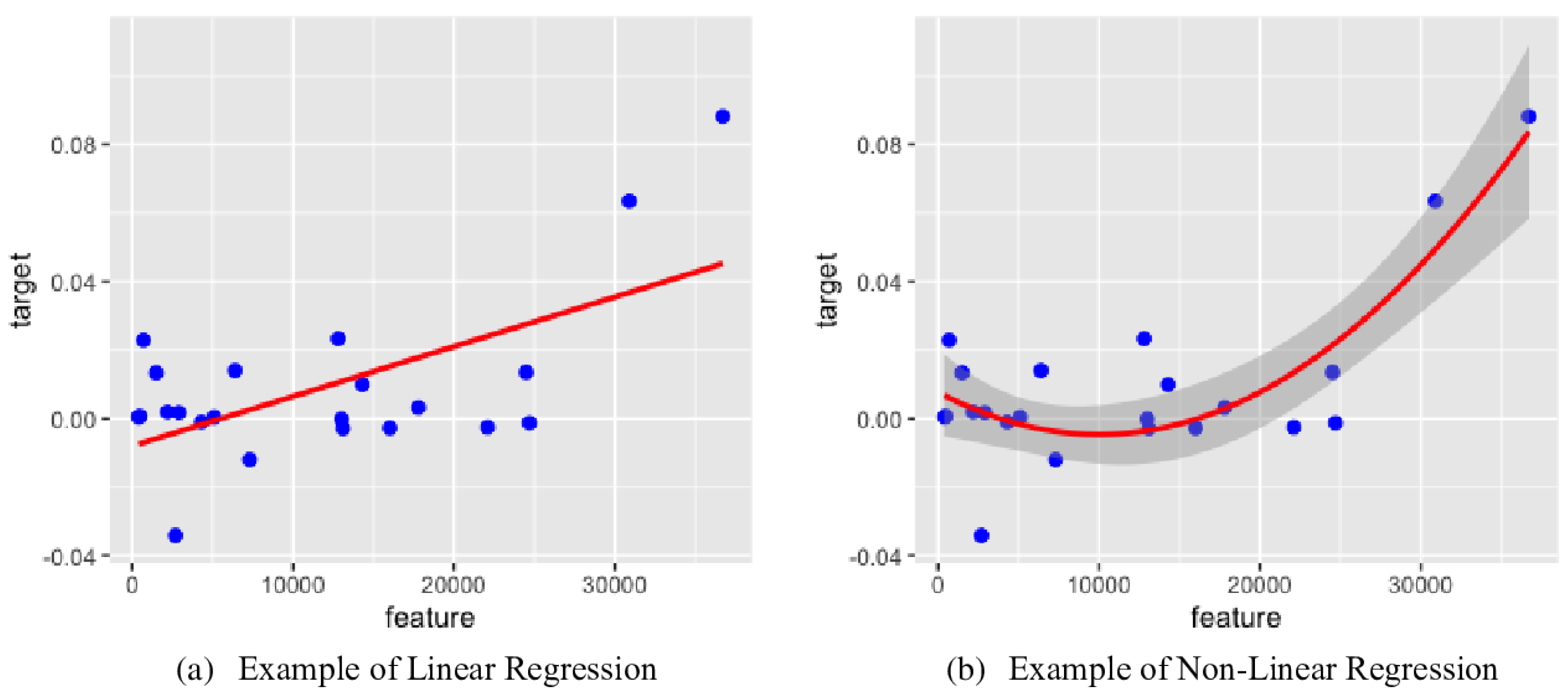
2.2. Polynomial Regression

2.2.1. Regression Model

Regression is a type of supervised machine learning. Regression is a method of analyzing the correlation between a given x and y and then predicting y based on the measured x. There are many types of regression analysis, but the most common are simple regression, multiple regression, and polynomial regression [13]. Simple regression analyzes the relationship between one independent variable and one dependent variable. Multiple regression is a technique for analyzing the relationship between a dependent variable and two or more independent variables. Unlike simple regression, it allows you to examine how multiple independent variables affect the dependent variable at the same time. It is used to analyze complex problems where multiple factors can affect the results. Polynomial regression analysis is a technique that models the correlation between the independent variable x and the dependent variable y as a curve using an nth-degree polynomial model. Due to its capacity to model complex nonlinear relationships, polynomial regression is extensively used across various fields, such as optimizing production processes, analyzing survival data, and managing energy systems. AbouHawa et al. used polynomial regression to model the intricate relationship between process parameters and product quality, predicting the optimal production conditions [14]. Oliveira et al. analyzed survival data to understand and predict the relationship between the survival rates of specific diseases or conditions and their covariates [15]. Xiong et al. conducted scheduling for an integrated energy system that takes into account the uncertainties of electricity, carbon, and gas prices, using polynomial regression to model price volatility over time and optimize energy production and consumption [16]. It is made by converting the independent variable of Equation (1) into the nth-order term with generalized multiple regression.

$$y=w_0+w_1{x}^1+w_2{x}^2+\dots +w_n{x}^n$$

(1)

The independent variable x is a variable that is not affected by other variable values and represents the cause. The dependent variable y is a variable that is affected by the independent variable and represents the result. In machine learning, the independent variable x is used as a feature and the dependent variable y is used as target data. $w_k(k=1\cdots n)$ represents the slope of x as a regression coefficient and weight in machine learning. $w_0$ is the intercept and bias in machine learning. $w_k$ is calculated based on the measured data, i.e., the training data.

In this paper, we use multiple quadratic polynomial regression. Therefore, converting Equation (1) into multiple quadratic polynomial regression results in the following Equation (2) [17].

$$\begin{array}{cc}\hfill y& =w_0+\sum _{j=1}^p{w}_j{x}_j+\sum _{j=1}^p\sum _{k=j}^p{w}_{j,k}{x}_j{x}_k\hfill \\ \hfill & =w_0+w_1{x}_1+w_2{x}_2+\cdots +w_p{x}_p+w_{1,1}{x}_1^2+w_{1,2}{x}_1{x}_2+\cdots \hfill \\ \hfill & +w_{1,p}{x}_1{x}_p+w_{2,2}{x}_2^2+w_{2,3}{x}_2{x}_3+\cdots +w_{2,p}{x}_2{x}_p+\cdots \hfill \\ \hfill & +w_{p-1,p-1}{x}_{p-1}^2+w_{p-1,p}{x}_{p-1}{x}_p+w_{p,p}{x}_p^2\hfill \end{array}$$

(2)

Here, $w_0$ is a constant, $w_j$ is the coefficient for linear terms, and $w_{jk}$ is the coefficient for pure quadratic and interaction terms. Additionally, p represents the number of independent variables, also known as features.

2.2.2. Model Optimization Algorithm

The regression model is optimized using methods such as OLS (Ordinary Least Squares) and gradient descent. The OLS method enhances the model’s prediction accuracy by minimizing the sum of squares of the residuals. The process of optimizing the parameters of a multiple quadratic polynomial regression model with n data points through OLS can be summarized as follows:

• Matrix (Vector) Transformation: The model is expressed in matrix form to encapsulate the linear, quadratic terms, and interaction terms for five features ($p=5$) based on Equation (2). The regression coefficients are organized in a vector W ([21 × 1]) as:

  $$W=\left[\begin{array}{c}{w}_0\\ w_1\\ ⋮\\ w_5\\ w_{1,1}\\ ⋮\\ w_{2,5}\\ ⋮\\ w_{5,5}\end{array}\right]$$
  For all n observations, the matrix X that includes five independent variables, their squares, and interaction terms is defined as the [n × 21] matrix as follows:

  $$X=\left[\begin{array}{cccccccccc}1& x_{1,1}& x_{1,2}& x_{1,3}& x_{1,4}& x_{1,5}& x_{1,1}^2& x_{1,1}{x}_{1,2}& \cdots & x_{1,5}^2\\ 1& x_{2,1}& x_{2,2}& x_{2,3}& x_{2,4}& x_{2,5}& x_{2,1}^2& x_{2,1}{x}_{2,2}& \cdots & x_{2,5}^2\\ ⋮& ⋮& ⋮& ⋮& ⋮& ⋮& ⋮& ⋮& \ddots & ⋮\\ 1& x_{n,1}& x_{n,2}& x_{n,3}& x_{n,4}& x_{n,5}& x_{n,1}^2& x_{n,1}{x}_{n,2}& \cdots & x_{n,5}^2\end{array}\right]$$
  And the dependent variable vector Y for all n observations is:

  $$Y=\left[\begin{array}{c}{y}_1\\ y_2\\ ⋮\\ y_n\end{array}\right]$$
  The model in matrix notation is then expressed as:

  $$Y=X·W$$
• Calculation of Least Squares Estimator: The optimal regression coefficient matrix W, known as the least squares estimator, is calculated by solving:

  $$\widehat{W}={(X^T·X)}^{-1}·X^T·Y$$

  where ${(X^T·X)}^{-1}$ is the inverse of the matrix product $X^T·X$, and $X^T$ is the transpose of X. This yields the least squares estimates for the regression coefficients.

2.2.3. Evaluation Metrics

When evaluating the prediction accuracy of regression models, the RSE or RMSE can be used to assess the performance of the model. The RSE is an estimate of the standard deviation of the residuals (errors) in the regression model. It quantifies the model’s lack of fit to the actual data points. Lower RSE values indicate a better model performance. The RSE can be calculated using the following Equation (3), where n is the number of data points, p is the number of independent variables used in the model, $y_i$ represents the actual observed values, and ${\widehat{y}}_i$ represents the predicted values by the model.

$$\mathrm{RSE}=\sqrt{\frac{1}{n-p-1}{\displaystyle \sum _{i=1}^n}{(y_i-{\widehat{y}}_i)}^2}$$

(3)

RMSE is an indicator used to measure the prediction error of a regression model, which is the square root of the average of the squared differences between the predicted values and the actual values. It is the square root of MSE (Mean Squared Error). While MSE averages the squares of errors, potentially overestimating the magnitude of errors, RMSE adjusts this by bringing the error magnitude back to its original units, making it more intuitive to understand. RMSE is calculated through Equation (4), where $y_i$ are the actual values, ${\widehat{y}}_i$ are the predicted values, and n is the number of observations.

$$\mathrm{RMSE}=\sqrt{\frac{1}{n}{\displaystyle \sum _{i=1}^n}{(y_i-{\widehat{y}}_i)}^2}$$

(4)

We evaluate the polynomial regression model using these two metrics: RSE assesses how well the model has learned from the training data, and RMSE checks the model’s accuracy on the test data. Since a model can still perform poorly if not properly trained, we use both RSE to confirm the model’s fit and RMSE to verify its accuracy simultaneously.

3. Proposed Methodology: Predicting OSS Survivability with Maintenance Activity

In this paper, we focus on estimating the OSS maintenance by emphasizing the risk of project dependencies. To achieve this, we use polynomial regression to predict OSS bug-fixing activity. Specifically, research is conducted on those with activity records within the last 2 years. This is because, after more than 2 years of inactivity, maintenance discontinuation can be determined without analysis. Previous research has primarily focused on estimating the current maintenance status of OSS. However, we employ trends in bug-fixing activities over time to identify future maintenance prospects. Trends indicate the direction of data, and trend calculations based on time-series data allow us to infer the increase or decrease in bug-fixing activities over time, making them a valuable factor in predicting bug-fixing activity trends. Our research is conducted in three steps, as shown in Figure 1. We describe the details of each step below.

3.1. Feature and Target Data

To predict bug-fixing activity, we use data related to popularity, contributors, and code complexity, as shown in

Table 2. Feature and target data.

	Type	Name	Description
Feature	User	Star	Interest level of open source users
	Developer	Contributor	Measure of development and maintenance activities.
	Code	LoC (line of code)	Project size
		Cognitive complexity	Developers’ code comprehension
		Cyclomatic complexity
Target	Maintainability	$Tren{d}_{bug}$	Bug-fixing activity

. To focus on the issue of project dependencies, we set bug-fixing activity as a maintenance criterion. It requires the identification of bugs by users and their resolution by developers. Moreover, for developers to efficiently maintain the project, the code should be easy to understand. Therefore, we utilize five types of data falling into three categories.

Star represents the number of stars in an open source repository. Stars go up when GitHub users are interested in a repository, so they represent the popularity of the repository [18,19]. The more popular a repository is, the more people are interested in it and the more likely it is to have users. Therefore, we use stars as user-side data.

Contributor is the number of people who contribute to the development of an open source repository. The more people contribute, the fewer features need to be developed and the fewer bugs need to be fixed per contributor. Therefore, the more contributors there are, the more likely it is that maintenance will be performed quickly and continuously, even if there are more bugs to fix. Therefore, we use contributor as a feature.

LoC (Line of Code) comprises data that indicate the size of a project. Based on research from [20], we found that a higher LoC require more maintenance effort. Based on this fact, we chose code as the data representing LoC because it can also affect the maintenance activity of bug-fixing.

Cognitive complexity is a metric that indicates the degree to which a person can understand code [21]. It is used to measure how much logical thought and cognitive work is required to understand and manage code from a developer’s perspective. In other words, it is an indicator of the intellectual burden of understanding code. Code with high cognitive complexity can be difficult to understand and harder to find and fix bugs, which can reduce the readability and maintainability of the code. That is why we use it as a feature.

Cyclomatic complexity is one metric of code complexity and is measured by analyzing the control flow of the code [22]. High cyclomatic complexity can increase the likelihood of bugs. We use this as a feature because it can affect the growth of bugs and increase maintenance efforts.

Target is the $Tren{d}_{bug}$. The trend indicates the increase or decrease in the number of residual bugs over time. Kenmei et al. and Akatsu et al. analyzed the state of OSS through issue creation and resolution progress [23,24]. We adopt this approach and use the trend of bug issue activity as the target to focus on bug resolution activity. Additionally, we calculate the trend value to quantitatively represent the current state of the OSS. If the value is above 0, it means that the number of residual bugs may increase in the future, indicating a higher risk of exposure to bugs due to a decrease in bug activity. Therefore, we adopt this as a criterion for identifying maintenance issues as it can indicate the risk of project dependency problems.

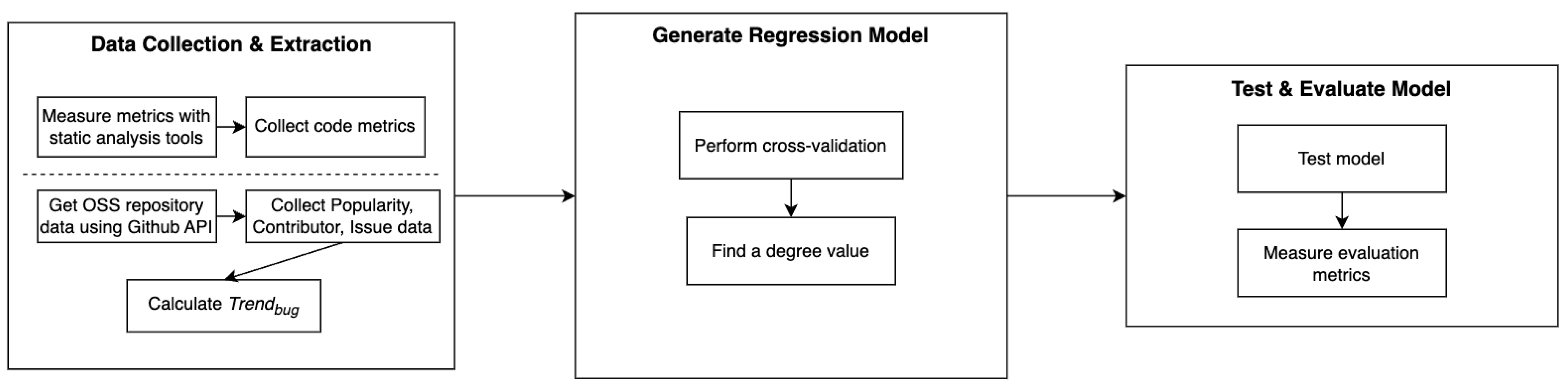
3.2. Data Collection and Extraction

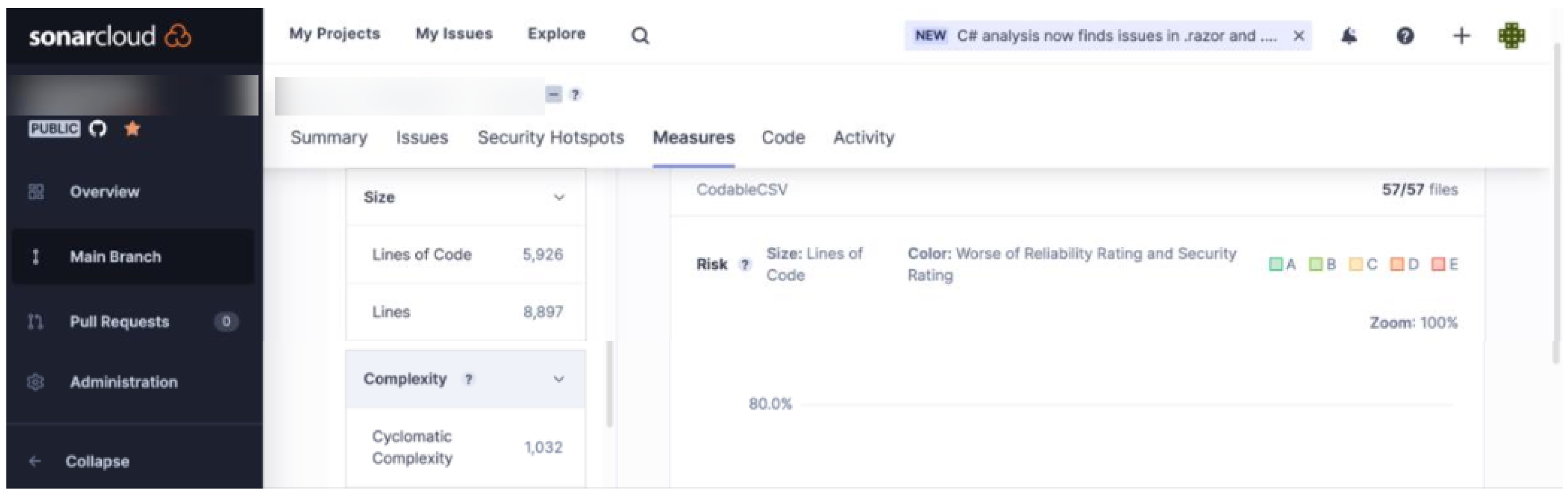
3.2.1. Collecting Feature Data

To collect feature and target data from the projects, we use the OSS repository page, PyGithub as GitHub API based on Python, and SonarCloud [25]. We then use R to convert the residual number of bug issues in the collected data into the targets in Table 2. We obtain data for features such as Star and Contributor from the data presented in Figure 2.

The LoC, cognitive complexity, and cyclomatic complexity of the code type were extracted using a static analysis tool called SonarCloud. After we uploaded the projects for analysis, we collect the analysis results as shown in Figure 3.

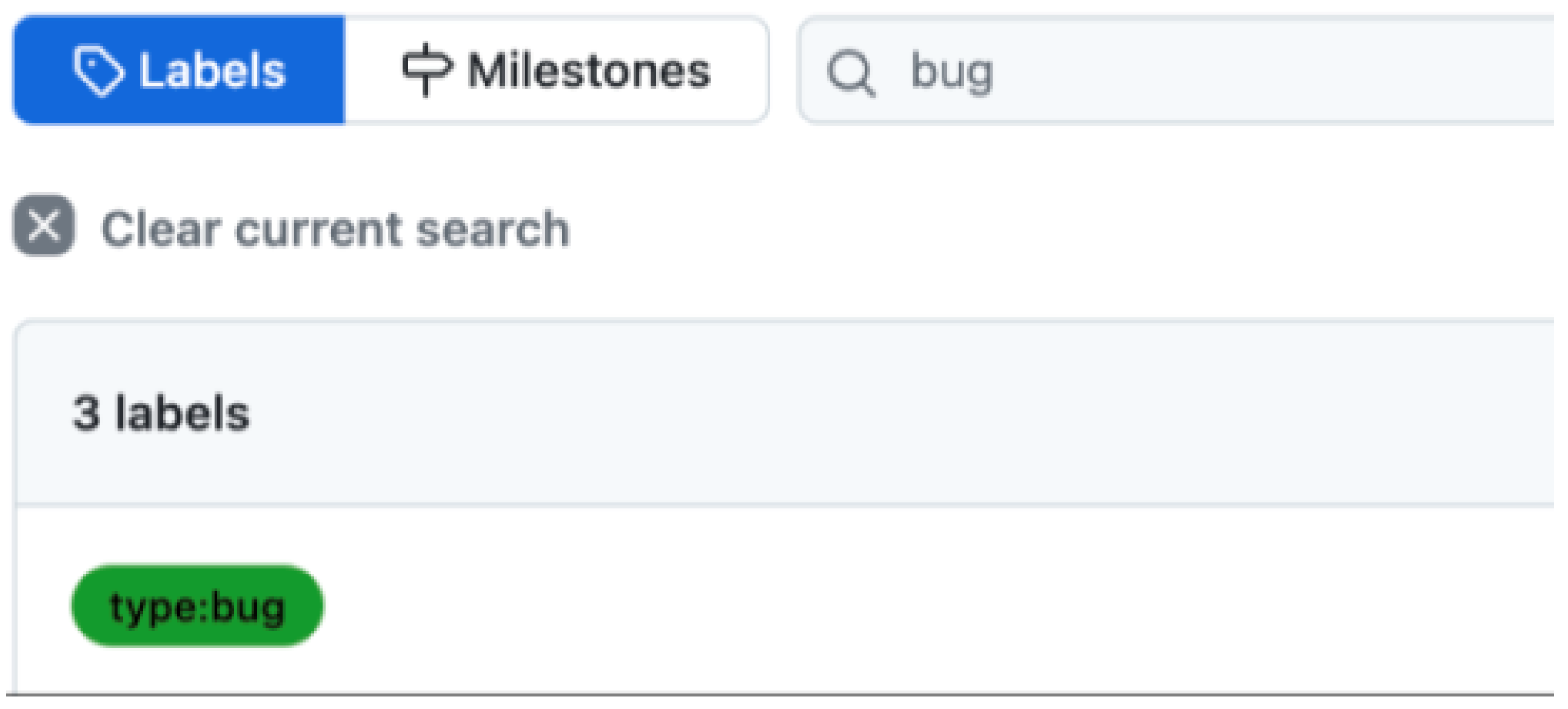
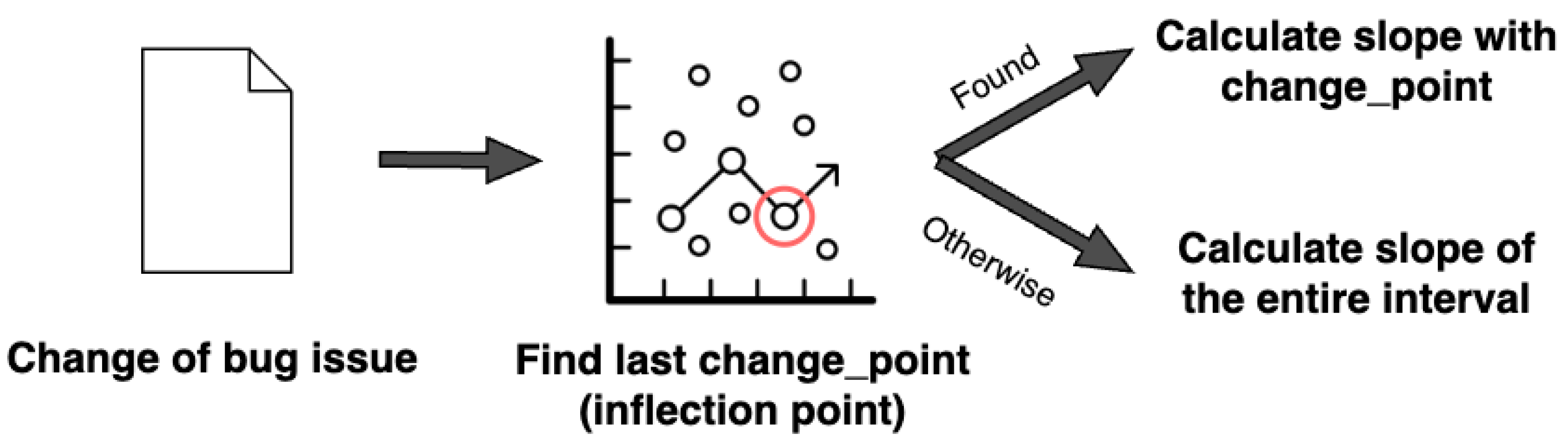
3.2.2. Extracting Target Data

The $Tren{d}_{bug}$ for the target was calculated using GitHub’s issue activity. Testing each project to identify the presence and fixing of bugs would require a considerable amount of time. Therefore, we used GitHub’s issue activity to determine the existence and fixing of bugs. When users or developers discover a bug, a bug issue is created. When a developer fixes the bug, the related issue is marked as closed. Hence, by tracking created bug issues and closed issues, we can determine the total number of bugs and the frequency of bug-fixing activity for OSS.

We utilize the GitHub API to extract issues. However, GitHub issues include not just bug-related problems but also questions regarding simple usage. To exclusively extract bug issues from the multitude, we search for labels categorized under ’bug’ as illustrated in Figure 4. Subsequently, leveraging the identified labels, we cumulatively gather created bug issues created and closed bug issues over the past two years, day by day. Thereafter, we compute the number of remaining bug issues for each date by comparing the two sets. Consequently, if bug issues are created but not closed, the count of remaining bug issues will incrementally rise over time. Alternatively, if more are closed than created within a two-year span, the quantity of remaining issues will progressively decrease.

Based on the collected data, we calculate the $Tren{d}_{bug}$ using Equation (5) to represent the trend of the data. However, the data do not exhibit an overall decrease or increase over the two-year period. It may show a decrease in some segments and an increase in others. Therefore, we used the code in Algorithm 1 to identify the last segment with a changing slope and utilized the slope of that segment as the target. For a comprehensive understanding of this process, please see Figure 5.

Algorithm 1 Calculating the slope of the last segment

Require: Use library $changepoint$ as $cpt$  $input\leftarrow OSS\left(date\right)$  $output\leftarrow OSS(residual\_bug\_issue)$  $change\_point\leftarrow cpt.mean\left(output\right)$  $slope\leftarrow calculate\_slope(input,output,change\_point)$  if $slope$ is NA then     $slope\leftarrow calculate\_slope(input,output)$  end if

Algorithm 1 operates using the changepoint library of R. After importing the necessary libraries, it takes the input of each OSS, which includes date, and the output, which consists of residual bug issues. Subsequently, the library is used to find the change_ point where the slope changes and calculate the slope of the last segment. In some cases, the slope value may remain constant over the entire segment. Therefore, in such cases, the calculation is performed over the entire segment.

$$Tren{d}_{bug}=\frac{{\sum }_j{(x}_j-\overline{x})(y_j-\overline{y})}{{\sum }_i{\left(x_i-\overline{x}\right)}^2}$$

(5)

Equation (5) calculates the rate of change of each piece of data over time, where x represents the date x when the issue was created or closed, and y represents the number of residual bugs. Based on the calculated trends, we can quantify the progress of bug-fixing activities in OSS in the future.

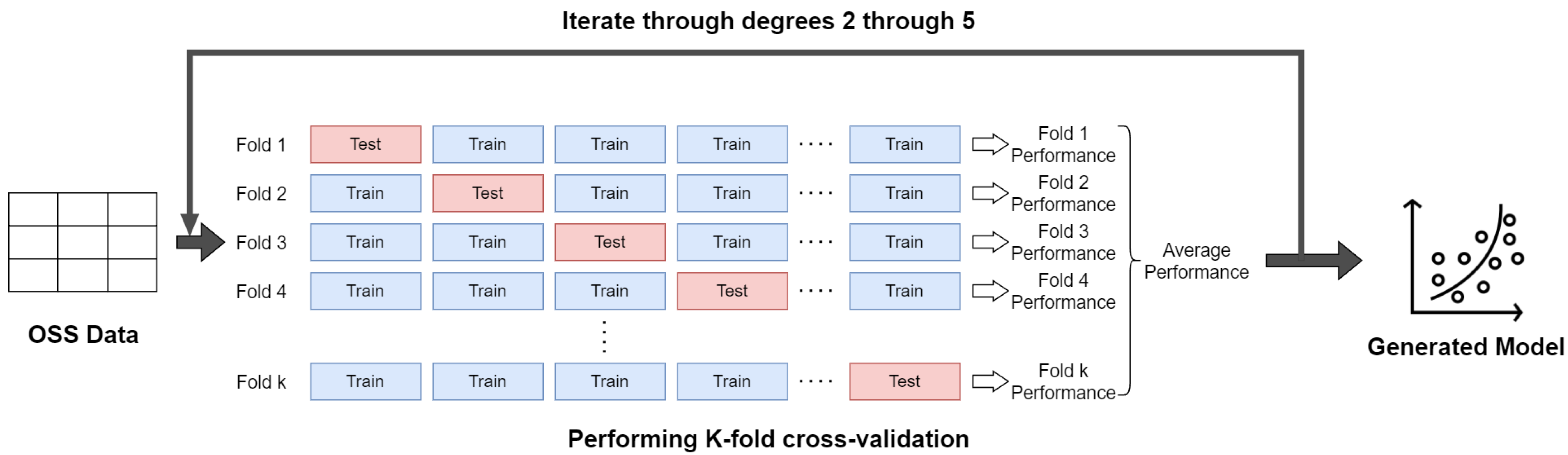
3.3. Generating Regression Model

In this paper, we employ polynomial regression to forecast bug-fixing activities for several key reasons. Firstly, our objective is to predict numerical values, necessitating a regression model over classification approaches. Polynomial regression, capable of capturing the curved relationships among data points due to its polynomial basis, is particularly suited for our second reason: the potential nonlinear relationships between various metrics and $Tren{d}_{bug}$. Lastly, given the manageable number of features in our dataset, the model complexity remains low, making polynomial regression an intuitive choice. We opt for polynomial regression over linear models to mitigate increased prediction errors and inaccuracies in capturing complex data patterns [26]. Linear models, typically designed to fit data in a straight line, often fail to accurately predict values at the extremes, either significantly higher or lower than most data points. This limitation is visually represented in Figure 6, which contrasts the fitting capabilities of linear and nonlinear regression models for the ‘Star’ feature and its impact on the target variable. The figure underscores the inadequacy of linear models for nonlinear data, thereby justifying our preference for polynomial regression to enhance model accuracy through its inherent nonlinearity.

To determine the degree of the polynomial, we evaluate the model across a range of degrees from 2 to 5, selecting the degree with the minimum RSE. Our research focuses on predicting the current and future survivability of OSS selections. Given the vast number of them, each with unique characteristics, our model must provide accurate results across diverse datasets. Since the RSE represents the model’s error on the data, minimizing the RSE serves as the criterion for selecting the degree. Additionally, our goal is to capture the overall trend of the target through the model. Therefore, we limit the degree to 5 or less to capture general data changes rather than aiming for exact fitting.

When training our model, we employ cross-validation. Cross-validation is a technique used in machine learning to reliably evaluate the performance of a model and estimate its generalization ability by repeatedly evaluating the model on the different subsets of the given data, dividing it into training and testing sets [27]. This technique aids in estimating generalization ability, preventing overfitting, and selecting the optimal model. Additionally, it is useful for assessing model quality when the dataset is small. With a limited amount of test data, the reliability of model quality measurement might decrease. Therefore, we employ cross-validation to evaluate the model across multiple training–test dataset splits and enhance the reliability of the model quality by averaging the results.

Cross-validation includes K-fold cross-validation, leave-one-out cross-validation, stratified cross-validation, time series cross-validation, and group cross-validation [28]. Among these, we opt for the first method. K-fold cross-validation involves dividing the data into k folds (subsets) as illustrated in Figure 7, using each fold as the test data while the rest serve as the training data to evaluate the model. Subsequently, as shown in Equation (6), this process is repeated k times to calculate the average performance of the model. Other methods are typically used for time series data, class imbalance, or grouped data. Since our conditions do not align with these criteria, we choose K-fold cross-validation.

$$\theta =\frac{1}{k}\sum _{i=1}^k{\theta }_i\left({\theta }_{i}isperformanceofFoldi\right)$$

(6)

The entire process of creating this model is summarized in Algorithm 2 and Figure 8, which is implemented in R. Initially, the feature and target data are loaded. Then, the data are divided into training and test sets. Next, to identify the appropriate degree of the polynomial, four models with degrees ranging from 2 to 5 are established, excluding degree 1 due to the nonlinear nature of the features, as demonstrated in Figure 6. Polynomial regression models are trained using the training data. Afterward, the models are evaluated using the test data, extracting the mean of RMSE and the mean of RSE. Based on these metrics, the model selection aims to prevent overfitting, adequately reflect the complexity of the data, and simultaneously optimize accuracy. This selection process seeks a balance between the model’s accuracy and complexity. The degree that minimizes the mean RSE is chosen, provided that the RMSE remains within an acceptable range. This approach selects a model that can capture the nonlinear patterns in the data while minimizing the risk of overfitting.

Algorithm 2 Generating polynomial model

$target\leftarrow calculate\_slope(date,residual\_bug\_issue)$  $feature\leftarrow OSS\left(feature\right)$  $feature,target\leftarrow split(k,feature,target)$  $performanceisempty$  $average\_performanceisempty$  for $degree=2$ to 5 do        for $k=1$ to 4 do           $test\leftarrow feature\left[k\right]+target\left[k\right]$           $train\leftarrow Otherfeatureandtarget$           $model\leftarrow polynomial\_regression(train,degree)$           $Addcalculate\_performance\left(model\right)toperformance$        end for        $Addaverage\left(performance\right)toaverage\_performance$  end for  return  $max(average\_performance)$

4. Results and Analysis

4.1. Target Application

To assess our proposed method, we utilized OSS employed in KakaoTalk. It is a mobile messenger app in South Korea, with approximately 50 million users, corresponding to a market share of 94.4%. We selected OSSs used in this application to focus on it commonly used in real software products. The iOS version of KakaoTalk employs a total of 121 OSS projects. However, we restricted our selection to those with recent open source activity within the last 2 years, resulting in the selection of 24 OSS projects meeting this criteria. Other environmental factors were set, as shown in

Table 3. Experiment dataset and model configuration.

Environmental Factors	Input Data
OSS source	KakaoTalk
Data collection period	∼30 September 2023
Total number of OSS	24
Learning method	Cross-validation
Cross-validation iterations (k)	4
Training data (by 1 iteration)	18
Testing data (by 1 iteration)	6
Degree	2
Optimization algorithm	OLS

.

As shown in

Table 4. Model evaluation results by degree 2–5.

Metric	Degree 2	Degree 3	Degree 4	Degree 5
Mean of RMSE	1.3100	99.6080	83,642.7561	33,254,864.4670
Mean of RSE	0.0101	0.0056	5.4098	2.5035

, after constructing and evaluating models with polynomial degrees of 2 to 5, it was found that all degrees except 2 exhibited very high RMSE values, indicating a high level of error. Furthermore, the degree of 2 showed the lowest RSE value, which means that the model represents the variability between features and the target well. Therefore, we set the model degree to 2.

4.2. RQ1: Experiment Results

To address RQ1, we analyzed the condition of OSS predicted to deteriorate based on survivability forecasts. Furthermore, we compared the survivability and condition of each OSS to identify the factors influencing the outcomes. The analysis of five OSS projects is depicted in Figure 9, which illustrates the changes in the number of remaining bugs over time for each OSS. Additionally, information regarding these OSS projects is presented in

Table 5. GitHub data of OSS in a state of maintenance deterioration.

Name	Age	Number of Contributors	Number of Residual Bugs	Number of Contributors (Last 1 Month)	Number of Commits (Last 1 Month)
CocoaPods	12	316	53	3	13
CodableCSV	5	11	1	0	0
normalize.css	12	45	0	0	0
Realm SwiftLint	8	354	47	14	72
Sentry Cocoa SDK	7	81	46	4	61

.

Among the five OSS projects, CodableCSV exhibited the highest $Tren{d}_{bug}$ value, indicating a significant decrease in bug-fixing activities or an increase in bug issues compared to other OSS, leading to the lowest survivability among the five. Table 5 shows that CodableCSV had the lowest number of contributors among the five OSS projects. Despite being one of the oldest OSS in the group, normalize.css recorded the lowest metrics. However, like CodableCSV, it has no currently active contributors, yet the two exhibited significant differences. The reasons for these differences, as identified through our analysis, are as follows:

• normalize.css is over twice as old as CodableCSV, which may have led to a slower decline in community and development activities, resulting in less fluctuation in activities and a lower trend.
• Compared to CodableCSV, normalize.css has approximately 150 times more forks and 10 times more stars. These characteristics contribute to the differences in GitHub issue activities between the OSS projects. CodableCSV has fewer new issues and a similarly low pull request activity. In contrast, normalize.css continues to generate a significant number of issues and, accordingly, more pull requests. Therefore, while CodableCSV might not be maintained further due to a lack of users and contributors, normalize.css seems more likely to find individuals to continue its legacy due to sustained interest.

Realm SwiftLint has been around for 8 years, CocoaPods for 12 years, and Sentry Cocoa SDK for 7 years, all considered to be relatively old but predicted similar metrics. The presence of currently active contributors in these three projects seems to prevent their $Tren{d}_{bug}$ from appearing high. However, despite being as old as normalize and having active contributors, CocoaPods showed a higher $Tren{d}_{bug}$ value, likely due to generating bug issues more frequently and quickly than normalize.css. Based on these metrics, if one were to choose an OSS for replacement, CodableCSV, which displayed the highest $Tren{d}_{bug}$, should be selected. The current status of each OSS is as follows:

CocoaPods is a library for managing dependencies in Xcode projects, developed over 12 years. It currently has three active developers, with 13 commits made last month. However, there are about 53 unresolved bug issues, and numerous issues continue to be reported. The high number of unaddressed issues suggests a lack of sufficient contributors to manage the workload.

CodableCSV is a library offering comprehensive functionality for reading/writing CSV files, developed over 5 years. However, it currently has no active contributors, leading to a complete halt in commit activities. As the system’s versions continue to increase, the likelihood of it failing to keep up with these versions also increases.

normalize.css is a library created 12 years ago to enable browsers to render all elements more consistently. As indicated in Table 5, it currently has no commit activity and lacks contributors, presenting a risk similar to CodableCSV of failing to adapt to later upgraded versions.

Realm SwiftLint, a tool for enforcing Swift style and conventions, was created 8 years ago. It has had 14 active contributors in the past month, which is relatively high compared to other OSS. However, with 47 unresolved bug issues and release update periods that have been extending beyond the initial monthly schedule, there is a risk of delayed bug fixes and prolonged exposure of the project to bugs.

The Sentry Cocoa SDK is an open source tool for automatic error monitoring in IOS applications, and it has been developed for 7 years. Its popularity, as shown in Table 5, is approximately 90% lower than the average popularity of other OSS projects used in the experiment, with #Star of 706. Additionally, there are 46 unresolved bug issues in the current repository, some of which have remained unresolved for as short as two days and as long as two years. Furthermore, the number of contributors, excluding bots, is currently at 4, and if their numbers decrease further, it could pose a challenge to the maintenance of the OSS.

In summary of the analysis, all five OSS currently exhibit either slow or nonexistent bug-fixing activities. Shorter-term projects have been found to have completely ceased development. For the remaining long-term projects, there is a buildup of unresolved bug issues from the past, coupled with the continuous addition of new bug issues, indicating a deterioration in maintenance. The trend in bug issue activity serves as an indicator of maintenance activity for these OSS projects.

Furthermore, these data provide meaningful insights for both open source users and administrators. For those planning to use OSS, opting for projects with high survivability can help reduce maintenance costs. Dependency on a specific open source project during development may lead to the code being tightly coupled to it. Subsequently, if the service of the open source project is discontinued, significant time and resources may be required to modify the related code. Therefore, for situations where the choice of open source has not been finalized, this insight can be helpful in reducing such costs.

Moreover, if using an open source project with low survivability, preparations can be made before its discontinuation. Unexpected service discontinuation can lead to swift modifications and significant expenses. By predicting low survivability in advance, alternative open source options can be explored, or functionalities can be developed directly to mitigate dependency issues with the concerned open source project.

Lastly, administrators wishing to sustain open source projects can be aware of their project’s status and exercise caution. Identifying the need for increased contributor engagement or community activation can help extend the project’s longevity by addressing issues in maintenance activity.

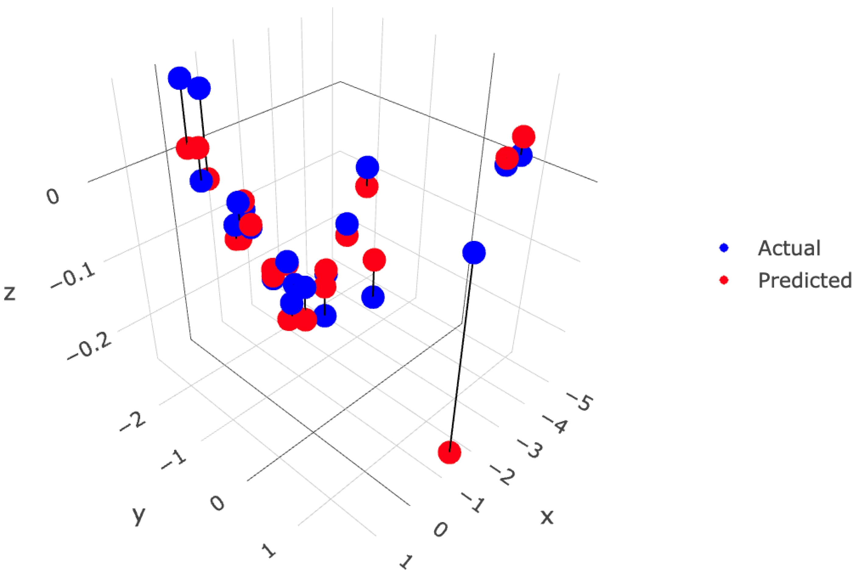
4.3. RQ2: Model Evaluation

To address RQ2, we evaluated our model using RSE and RMSE. Since MSE calculates the average of the squares of errors, it may overemphasize errors, making it preferable to use RMSE for assessing the accuracy of the model. RMSE, being the square root of MSE, rescales the magnitude of errors to their original units, allowing for a more intuitive understanding of model accuracy. RSE represents the standard deviation of the errors, taking into account the complexity of the model. An increase in RSE value indicates lower consistency in predictions. For these reasons, we use RSE to assess the model’s fit, i.e., how well it has learned from the given data. Since a model can be inaccurately measured for accuracy if not properly trained, we assess its fit using RSE. These metrics were extracted for each fold through performing K-fold cross-validation. The results of the evaluation are presented in

Table 6. Model evaluation results using K-fold cross-validation.

Metric	Fold 1	Fold 2	Fold 3	Fold 4	Mean
RMSE	5.0024	0.1810	0.0350	0.0215	1.3100
RSE	0.0099	0.0098	0.0142	0.0067	0.0101

.

Upon reviewing Table 6, a consistent pattern of low RSE values, with an average of 0.0101 across all folds, indicates that the model effectively captures the variability of the dataset. However, the RMSE values exhibit considerable variability, notably with an outlier in fold 1. To further analyze these figures, visualization was performed through Figure 10. Using SVD (Singular Value Decomposition) for PCA (Principal Component Analysis), we reduced five-dimensional data to two dimensions to create a three-dimensional graph, as mentioned in [29]. SVD is a numerically very stable decomposition method, which is more robust against errors that can occur in floating-point arithmetics, hence the choice of SVD over eigenvalue decomposition. X and Y represent the data reduced via SVD, while Z is the target variable, $Tren{d}_{bug}$. The figure shows that some data were predicted lower than their actual values, leading to an increased RMSE value in Fold 1. While the rest of the data did not match perfectly, they were predicted quite closely. In contrast, Folds 2, 3, and 4 displayed significantly lower RMSE values of 0.1810, 0.0350, and 0.0214, respectively, indicating strong compatibility between the model and the training and target datasets used in these folds. Consequently, the overall average RMSE slightly increased to 1.3100, compared to the lower values observed in Folds 2, 3, and 4. This discrepancy suggests that the test set used in Fold 1 included data points different from those used in the model’s training. Additionally, this implies that the training data in Fold 1 did not fully represent the test data.

In particular, the test set in Fold 1 included an OSS called Alamofire, which generally had higher feature values compared to other OSS, notably in metrics like popularity represented by stars. Consequently, the training set for Fold 1 lacked data points with high feature values, such as stars or other features, leading to inaccurate predictions when testing with this OSS and resulting in the relatively high RMSE value. Overall, while the model demonstrated good performance, the discrepancy in accuracy for certain folds indicates areas where further refinement is needed, highlighting the importance of dataset augmentation in future iterations.

4.4. Discussion

In this paper, we modeled the survivability of OSS using polynomial regression with features and targets as indicated in

Table 7. Comparison with Other Studies: Machine Learning Techniques.

	Our Study	Coelho et al. [8]	Zhou et al. [9]	Decan et al. [10]
Feature	Number of Stars and Contributors, LoC, Cognitive complexity, Cyclomatic complexity	Commit, fork, issue, pull request, number of consecutive days without commit, contribution by developer, etc.	3-tuple (event type, user group, time stamp) event type: any activity that may occur in the repository, such as create, delete, fork, issue, etc.	Previous and recent commit activities of each contributor
Target	$Tren{d}_{bug}$ (Trend of bug-fixing activities)	Release presence in the past month	Analyzes past repository activity data to forecast developmental changes	When contributors are next active
Technique	Multiple quadratic polynomial regression	Random forest	End-to-end multitasking sequential deep network	ARIMA (auto-regressive integrated moving average)

. Our approach distinguishes itself from the related studies in terms of feature composition and modeling aspects, as outlined in Table 7. Coelho et.al. focused on a classification model to differentiate between maintained and unmaintained projects [8]. In contrast, our research models survivability as a continuum, enabling more detailed predictions about a project’s health and long-term survival. Zhou et al. predicts the future state of a repository by analyzing its evolutionary trends, employing a deep learning-based analysis of time-series data and predicting activities like star counts and commits, requiring substantial data collection [9]. Our method, focusing solely on bug-fixing activities, requires less data and is less complex. Decan et al. focuses on predicting OSS commit activities, estimating the time elapsed until the next contribution based on individual contributors’ past and recent contributions, analyzing the time until an event occurs to estimate the next activity period [10]. This method, like Zhou et al., also depends on a model trained specifically for one OSS.

Additionally, all these studies considered both feature development and bug-fixing activities in assessing the OSS maintenance state, but they focused on overall development activities, limiting a clear understanding of the residual bug risk. Each study has its unique limitations. Coelho et al. used releases as a maintenance criterion, which has the limitation of not clearly presenting the current situation as releases accumulate over time [8]. In contrast, bug-fixing activities, based on the integration of current data, offer advantages in verifying current activities. Decan et al. focused on the sustainability of contributing activities [10], which is more useful for OSS management than for users considering OSS selection, where the criteria for selecting OSS remain unclear.

4.5. Threats to Validity

We proposed a method to predict the development process and trends of OSS using polynomial regression analysis based on GitHub data. We identified and addressed several potential threats to the validity of our findings. These threats are divided into two categories: external threats and internal threats, and each category has associated mitigation strategies.

External threats: Each OSS project may exhibit unique development patterns, influenced by factors such as the size and complexity of the project and the dynamics of the contributing community. Some OSS projects may follow a well-defined and predictable development pattern, making them good candidates for regression analysis to predict stability using the proposed method. However, some OSS projects may have a highly irregular development pattern, characterized by unpredictable changes, inconsistent bug-fixing activity, or other nonlinear trends. In these cases, traditional regression models may struggle to identify meaningful patterns, limiting the effectiveness of reliability prediction methods. To address these external threats, we used cross-validation to train the model on different subsets of the training data and evaluate the model’s performance. Furthermore, extracting only bug issues can be challenging if issue labeling is not performed. Therefore, we excluded those OSS from our study. However, if measuring survivability including them is necessary, methods used by Coelho et al. or Decan et al. might be more suitable [8,10].

Internal threats: The size of the dataset used to train and test a model can affect its performance. A small sample size can limit representativeness and reduce predictive accuracy. To address this insider threat, only open sources with sufficient data should be used. Therefore, we ran our predictions on open sources with at least five data points.

5. Conclusions

The adoption of OSS in modern software development is increasing, bringing both convenience and challenges. While OSS enhances development efficiency, it can also lead to problems such as project dependency due to maintenance discontinuation resulting from uncertain bug fixes. Consequently, software maintenance costs may rise, prompting users to consider long-term support and maintenance when choosing OSS. Previous studies have focused on OSS development activities or version support [8,9,10]. However, unlike these methods, we conducted research focusing on the maintenance status and survivability of OSS based on the activities of contributors and users.

In this paper, we proposed predicting OSS survivability using polynomial regression. We conducted research in three stages. In the first stage, data collection and extraction, we collected the characteristics of OSS users, contributors, and code that influence bug-fixing activities. Additionally, we calculated $Tren{d}_{bug}$, representing the bug-fixing activity, using the collected data and extracted target data. In the second stage, we performed K-Fold cross-validation for degrees 2 through 5 to identify the degree showing the highest performance and then created and selected the model. In the final stage, we predicted the survivability of OSS using the generated model and validated the results. We applied these three steps to 24 OSS used in KakaoTalk, confirming a predicted decrease in the survival potential of the majority of OSS. Upon examining the repositories of five OSS, it was observed that the maintenance activities such as delayed or discontinued release versions and decreased contributor participation were evident. This suggests that it would be beneficial to use things that have a high probability of survival to prepare for OSS deprecation.

We believe that our research can contribute to both OSS users and administrators. Firstly, OSS users can support the selection of OSS for cost savings in projects. Additionally, OSS administrators can receive warnings about the need for solutions to ensure project survival. However, there are still limitations to this method. Issues such as not distinguishing between areas of issues in various OSS and not promptly closing issues were observed. Therefore, careful consideration is needed when applying our method to understand its current state if proper management is not being carried out. To address these limitations, in future research, we aim to differentiate bug issues in different ways for more accurate predictions.

References

1. OpenLogic.com. 2022 Open Source Report Overview: Motivations for OSS Adoption. 2022. Available online: https://www.openlogic.com/blog/2022-open-source-report-overview (accessed on 6 March 2023).
2. Spinellis, D.; Szyperski, C. How is open source affecting software development? IEEE Softw. 2004, 21, 28–33. [Google Scholar] [CrossRef]
3. Lavallée, M.; Robillard, P.N. Why good developers write bad code: An observational case study of the impacts of organizational factors on software quality. In Proceedings of the 2015 IEEE/ACM 37th IEEE International Conference on Software Engineering, Florence, Italy, 16–24 May 2015; Volume 1, pp. 677–687. [Google Scholar] [CrossRef]
4. snyk.io. 5 Potential Risks of Open Source Software. 2023. Available online: https://snyk.io/learn/risks-of-open-source-software/ (accessed on 6 March 2023).
5. Mansfield-Devine, S. The secure way to use open source. Comput. Fraud. Secur. 2016, 2016, 15–20. [Google Scholar] [CrossRef]
6. Goodin, D. Extremely severe bug leaves dizzying number of software and devices vulnerable. ARS Tech. 2016. Available online: https://arstechnica.com/information-technology/2016/02/extremely-severe-bug-leaves- (accessed on 6 March 2023).
7. Spinellis, D. Choosing and using open source components. IEEE Softw. 2011, 28, 96. [Google Scholar] [CrossRef]
8. Coelho, J.; Valente, M.T.; Silva, L.L.; Shihab, E. Identifying unmaintained projects in github. In Proceedings of the 12th ACM/IEEE International Symposium on Empirical Software Engineering and Measurement, Oulu, Finland, 11–12 October 2018; pp. 1–10. [Google Scholar] [CrossRef]
9. Zhou, H.; Ravi, H.; Muniz, C.M.; Azizi, V.; Ness, L.; de Melo, G.; Kapadia, M. Gitevolve: Predicting the evolution of github repositories. arXiv 2020, arXiv:2010.04366. [Google Scholar]
10. Decan, A.; Constantinou, E.; Mens, T.; Rocha, H. GAP: Forecasting commit activity in git projects. J. Syst. Softw. 2020, 165, 110573. [Google Scholar] [CrossRef]
11. Samoladas, I.; Angelis, L.; Stamelos, I. Survival analysis on the duration of open source projects. Inf. Softw. Technol. 2010, 52, 902–922. [Google Scholar] [CrossRef]
12. Mari; Eila. The impact of maintainability on component-based software systems. In Proceedings of the 2003 29th Euromicro Conference, Belek-Antalya, Turkey, 1–6 September 2003; pp. 25–32. [Google Scholar] [CrossRef]
13. Ostertagová, E. Modelling using polynomial regression. Procedia Eng. 2012, 48, 500–506. [Google Scholar] [CrossRef]
14. AbouHawa, M.; Eissa, A. Corner cutting accuracy for thin-walled CFRPC parts using HS-WEDM. Discov. Appl. Sci. 2024, 6, 1–20. [Google Scholar] [CrossRef]
15. Oliveira, C.H.X.; Demarqui, F.N.; Mayrink, V.D. A Class of Semiparametric Yang and Prentice Frailty Models. arXiv 2024, arXiv:2403.07650. [Google Scholar]
16. Xiong, J.; Sun, Y.; Wang, J.; Li, Z.; Xu, Z.; Zhai, S. Multi-stage equipment optimal configuration of park-level integrated energy system considering flexible loads. Int. J. Electr. Power Energy Syst. 2022, 140, 108050. [Google Scholar] [CrossRef]
17. Yang, W.C.; Yang, J.Y.; Kim, R.C. Multiple Quadratic Polynomial Regression Models and Quality Maps for Tensile Mechanical Properties and Quality Indices of Cast Aluminum Alloys according to Artificial Aging Heat Treatment Condition. Adv. Mater. Sci. Eng. 2023, 2023, 7069987. [Google Scholar] [CrossRef]
18. Borges, H.; Hora, A.; Valente, M.T. Understanding the factors that impact the popularity of GitHub repositories. In Proceedings of the 2016 IEEE International Conference on Software Maintenance and Evolution (ICSME), Raleigh, NC, USA, 2–7 October 2016; pp. 334–344. [Google Scholar] [CrossRef]
19. Borges, H.; Hora, A.; Valente, M.T. Predicting the popularity of github repositories. In Proceedings of the 12th International Conference on Predictive Models and Data Analytics in Software Engineering, Ciudad Real, Spain, 9 September 2016; pp. 1–10. [Google Scholar] [CrossRef]
20. Hayes, J.H.; Patel, S.C.; Zhao, L. A metrics-based software maintenance effort model. In Proceedings of the Eighth European Conference on Software Maintenance and Reengineering, Tampere, Finland, 24–26 March 2004; CSMR 2004. pp. 254–258. [Google Scholar] [CrossRef]
21. Campbell, G.A. Cognitive complexity: An overview and evaluation. In Proceedings of the 2018 International Conference on Technical Debt, Gothenburg, Sweden, 27–28 May 2018; pp. 57–58. [Google Scholar] [CrossRef]
22. Ebert, C.; Cain, J.; Antoniol, G.; Counsell, S.; Laplante, P. Cyclomatic complexity. IEEE Softw. 2016, 33, 27–29. [Google Scholar] [CrossRef]
23. Kenmei, B.; Antoniol, G.; Di Penta, M. Trend analysis and issue prediction in large-scale open source systems. In Proceedings of the 2008 12th European Conference on Software Maintenance and Reengineering, Athens, Greece, 1–4 April 2008; pp. 73–82. [Google Scholar]
24. Akatsu, S.; Masuda, A.; Shida, T.; Tsuda, K. A Study of Quality Indicator Model of Large-Scale Open Source Software Projects for Adoption Decision-making. Procedia Comput. Sci. 2020, 176, 3665–3672. [Google Scholar] [CrossRef]
25. 2023. Available online: https://www.sonarsource.com/products/sonarcloud/ (accessed on 11 October 2023).
26. Maulud, D.; Abdulazeez, A.M. A review on linear regression comprehensive in machine learning. J. Appl. Sci. Technol. Trends 2020, 1, 140–147. [Google Scholar] [CrossRef]
27. Soper, D.S. Greed is good: Rapid hyperparameter optimization and model selection using greedy k-fold cross validation. Electronics 2021, 10, 1973. [Google Scholar] [CrossRef]
28. Ramezan, C.A.; Warner, T.A.; Maxwell, A.E. Evaluation of sampling and cross-validation tuning strategies for regional-scale machine learning classification. Remote Sens. 2019, 11, 185. [Google Scholar] [CrossRef]
29. Tanwar, S.; Ramani, T.; Tyagi, S. Dimensionality reduction using PCA and SVD in big data: A comparative case study. In Proceedings of the Future Internet Technologies and Trends: First International Conference, ICFITT 2017, Surat, India, 31 August–2 September 2017; Proceedings 1. Springer: Berlin/Heidelberg, Germany, 2018; pp. 116–125. [Google Scholar]
Figure 1. Detailed process flow for predicting OSS’ bug trends with polynomial regression.
Applsci 14 02812 g001
Figure 2. Example of feature data (star, contributor).
Applsci 14 02812 g002
Figure 3. SonarCloud: code data extraction.
Applsci 14 02812 g003
Figure 4. Issue label of GitHub.
Applsci 14 02812 g004
Figure 5. Example of performing Algorithm 1 (red circle denotes last changed point).
Applsci 14 02812 g005
Figure 6. Differences between linear and nonlinear regression.
Applsci 14 02812 g006
Figure 7. Process of performing K-fold cross-validation.
Applsci 14 02812 g007
Figure 8. Example of performing algorithm 2.
Applsci 14 02812 g008
Figure 9. Change in bug-fixing activities of OSS.
Applsci 14 02812 g009
Figure 10. Comparison of model prediction results using SVD (X, Y: compressed data, Z: target).
Applsci 14 02812 g010