Article

An End-to-End Deep Learning Framework for Predicting Hematoma Expansion in Hemorrhagic Stroke Patients from CT Images

1
Computer Vision and Robotics Group, University of Girona, 17004 Girona, Spain
2
Department of Neurology, Hospital Universitari Dr Josep Trueta, Institut d’Investigació Biomèdica de Girona, 17007 Girona, Spain
*
Author to whom correspondence should be addressed.
Appl. Sci. 2024, 14(7), 2708; https://doi.org/10.3390/app14072708
Submission received: 28 February 2024 / Revised: 18 March 2024 / Accepted: 22 March 2024 / Published: 23 March 2024

Abstract

:
Hematoma expansion (HE) occurs in 20% of patients with hemorrhagic stroke within 24 h of onset, and it is associated with a poorer patient outcome. From a clinical point of view, predicting HE from the initial patient computed tomography (CT) image is useful to improve therapeutic decisions and minimize prognosis errors. In this work, we propose an end-to-end deep learning framework for predicting the final hematoma expansion and its corresponding lesion mask. We also explore the problem of having limited data and propose to augment the available dataset with synthetic images. The obtained results show an improved HE prediction when incorporating the use of synthetic images into the model, with a mean Dice score of the HE growth area of 0.506 and an average prediction error in hematoma volume of 3.44 mL. The proposed approach achieved results in line with state-of-the-art methods with far fewer data by using synthetic image generation and without requiring the inclusion of patient clinical data.

1. Introduction

Stroke remains the second-leading cause of death globally, with 101 million prevalent cases in 2019 [1], and showed significant increases in its prevalence and incidence rates in people younger than 70 years between 1990 and 2019, with an even faster increase from 2010 to 2019. Among all stroke cases, 10–15% belong to intracerebral hemorrhage (ICH), which demonstrates greater mortality and morbidity rates [2]. In ICH, patient outcome is highly dependent on the final hematoma volume, which can grow since the time of admission and the first diagnostic imaging scan. Hematoma expansion (HE) is defined as a relative increase in hematoma volume > 33 % or an absolute increase > 6 mL [3]. It occurs in 30–38% of patients with ICH, and it can drastically worsen functional outcome and lead to disability and death [4]. For instance, for each 1 mL of absolute increase in hematoma volume, patients are 7% more likely to worsen from independence to poor outcome [5]. Therefore, it is crucial to rapidly identify patients at risk of HE at the time they present with intracerebral hemorrhage.
Computed tomography (CT) is the prevalent modality for hemorrhagic stroke diagnosis [6], as it is widely available and allows for rapid and inexpensive image acquisition. It can provide prognostic information that might help identifying patients at risk of HE. Nowadays, investigation of different imaging markers that could predict the expansion of hematoma is a trending research topic. Various radiological markers have been proposed; for instance, the spot sign, identified from CT angiography (CTA) images, is the most currently studied radiological predictor of HE [7,8]. However, the sensitivity of CTA spot sign to HE remains low, and CTA is not systematically performed for stroke diagnosis and may not even be available in some centers [8,9].
Additionally, several CT HE markers have been developed to predict the risk of HE. For instance, the blend sign is a relatively hypoattenuated area next to a hyperattenuated area of the hematoma, with a well-defined margin between the two regions [10]; the swirl sign is the presence of one or more rounded or irregular regions of hypoattenuation or isoattenuation within the hemorrhage [10]. Another HE imaging biomarker is the black hole sign, which is defined as a low-density area wrapped in the high-density area with an identifiable border [3]. Some other examples of HE prediction biomarkers are the island sign, hypodensity, and the satellite sign [9]. Even though these CT imaging markers seem to be promising for HE prediction, their clinical relevance and contribution to the field are still under investigation and require further research [3,9,11].
Current clinical practice suggests the acquisition of initial CT upon arrival of the patient to the hospital and then repetition of the scan within 24 h to evaluate the development of HE, particularly in patients that show neurological deterioration [11]. From a clinical point of view, it is relevant to predict HE growth from the initial image and, a more challenging yet valuable task, to predict the final HE of the lesion, which can provide more comprehensive information on the extent and pattern of its growth and facilitate better clinical decision making.
There are several research works predicting the final extent of the lesioned area in ischemic stroke [12,13]. However, to the best of our knowledge, there is only one work, developed by [14], which tackled the problem of hemorrhagic stroke growth prediction. Their approach is based on the assumption that the follow-up hematomas are based on the initial hematomas’ spatial characteristics and displacements. Their algorithm is a deep learning approach based on an encoder–decoder framework which learns a displacement vector field (DVF), which is used to warp the baseline CTs with the corresponding hematoma mask into the predicted follow-up image and its lesion mask. However, their approach includes also clinical metadata, which is incorporated into the model by using a specially designed metadata fusion block placed after the encoder branch of the network. In practice, there can be some limitations to maintaining this kind of approach, like lack of imaging and clinical data. As hemorrhagic stroke is less frequent than ischemic stroke and HE occurs in less than 40% of cases, it can be hard for researchers to collect reliable images for developing their algorithms. Moreover, despite clinical information being very helpful in HE prediction [15], some of it might not be available to the clinician right away together with the image.
Recently, synthetic images have been actively used for data augmentation, with many works showing that they can aid different medical image analysis approaches, especially in limited-data settings [16,17]. For instance, there are proposals to use synthetic images for cardiovascular region segmentation [18], liver tumor segmentation [19], brain lesion segmentation [20,21], brain atrophy quantification [22], and many other applications.
In this work, inspired by the main contributions of the seminal work proposed in [14], we develop a deep learning approach to predict hematoma growth in a limited-data setting and without requiring the inclusion of clinical data. We propose a 3D patch-based U-Net model which learns the deformation field from longitudinal CT images of hemorrhagic stroke lesions to then perform the prediction of the HE area by using only the initial patient CT image. To address the scarcity of data, we adapted the recent work of [23] to augment the initial training set with different synthetic variations in the baseline hematoma regions from the available cases and studied the impact of using these synthetic images to improve the prediction of the follow-up HE mask.

2. Materials and Methods

2.1. Dataset

The dataset used in this project consisted of 140 non-contrast head CT images acquired at Hospital Dr. Josep Trueta, Girona, Spain. The following inclusion criteria were applied: (1) patients older than 18 years; (2) diagnosis of acute spontaneous and anticoagulation-associated supratentorial ICH within 12 h of symptom onset; (3) informed consent was signed by the patient or relatives; (4) patient had both baseline and follow-up CTs; (5) patient had intraparenchymal hemorrhage only, excluding cases with other subtypes of stroke, like intraventricular hemorrhage; (6) hematoma volume in baseline image was not less than 5 mL; (7) the follow-up images should demonstrate HE as defined before, i.e., a relative increase in hematoma volume of >33% or absolute increase in volume of >6 mL. The exclusion criteria were the following: (1) known secondary ICH etiology (trauma or underlying vascular malformation), (2) surgical hematoma evacuation, (3) expectancy of life under 6 months, (4) pregnancy, and (5) suboptimal imaging acquisition. From the 140 cases, 27 matched the abovementioned criteria and were used to develop the proposed approach.
Hematoma masks in basal and follow-up images were obtained by using a semisupervised approach. An automatic deep learning approach [24] was first applied to obtain the initial hematoma masks, which were then manually refined by an expert neuroradiologist with 15 years of experience in hemorrhagic stroke. The same expert refined both the baseline and follow-up masks for each particular patient to avoid unwanted bias in HE determination.

2.1.1. Data Preprocessing

To focus our analysis on brain tissue regions, we performed skull stripping and coil removal on the initial CT image, as done in [24]. Both operations were performed by using morphological operations, like biggest connected component extraction for coil removal and a combination of different morphological operations for skull border elimination. Afterwards, baseline CT images were co-registered to the corresponding follow-up CT images, similarly to the study [14] (two rigid registrations followed by affine registration), and the corresponding masks were interpolated accordingly by using SimpleITK [25,26,27].

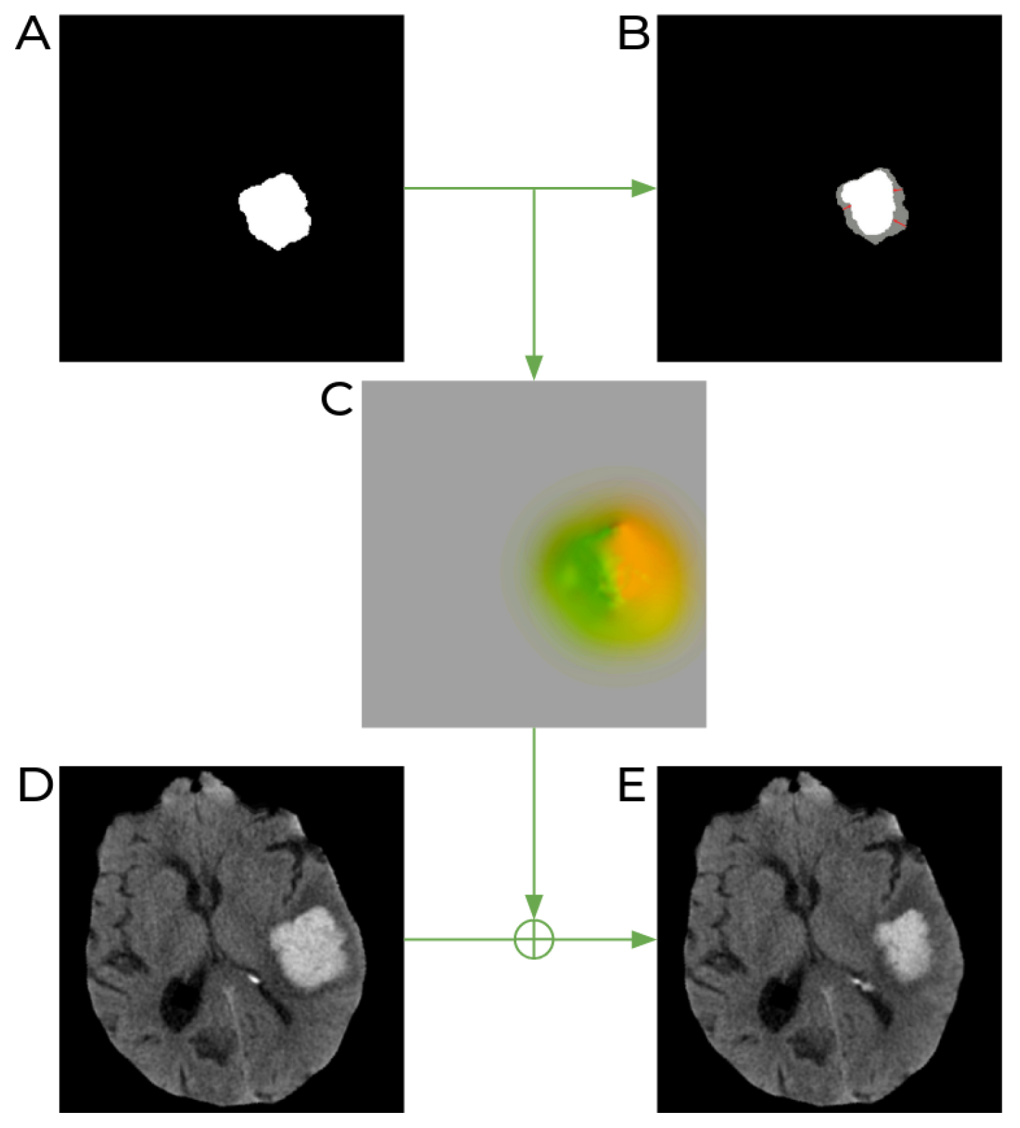
2.1.2. Synthetic Dataset Generation

To be able to tackle the scarcity of data, we propose to synthetically enlarge the dataset of baseline–follow-up image pairs presenting HE. We do so by utilizing the existing baseline images and introducing some variations in hematoma appearance, e.g., by slightly altering its shape, size, morphology, and intensity. The idea is to generate novel baseline images without losing the main information regarding the hematoma growth pattern.
Our image synthesis is inspired by the work of [23], where the authors propose an approach to produce synthetic cortical atrophy, generating a longitudinal ground-truth dataset specifically designed for accuracy validation of surface-based CT measurements. Following the same procedure, we apply slight deformations to the baseline hematoma to obtain different versions of the lesion, while preserving the same follow-up image in order to keep the expansion behavior as much as possible.
To achieve this, we follow several steps, as shown in Figure 1. The first one is to generate the target hematoma mask, which will represent our desired lesion appearance in one of the variants of the baseline image. Similarly to the work of [23], we utilize morphological operations for this purpose, using different binary morphological operations (with only 1–2 iterations) to introduce small changes in the baseline hematoma mask (see Figure 1). For our task of predicting hematoma expansion, we generate 5 different versions of each baseline image, to produce more baseline–follow-up image pairs for training. All of them are produced using the same binary erosion operation but with different 3D structuring elements of dimensions 3 × 3 × 3 , which are chosen randomly and some of which are repeated two times. This way, the final mask of each new version is slightly different from all the other masks of the same case (and between different patients), avoiding repetitive patterns or biasing the training data, which could affect the models.
Once this step is complete, we move to the second stage and calculate a transformation to deform the baseline image accordingly. Following the same approach as in [23], we achieve this by deformably registering the original baseline mask to the eroded one by using the publicly available Greedy software [28]. This results in a deformation field from the real baseline to the desired one (see Figure 1C). In the third step, we apply this resulting deformation field to the original baseline CT image to artificially shrink the hemorrhagic stroke lesion (Figure 1E). The intensities in the resulting image are obtained with linear interpolation. Finally, our training set includes 6 baseline–follow-up pairs generated from one patient: the original pair and 5 more pairs where the baseline lesion has a different appearance. Note that the follow-up images are the same for all the pairs within the same patient.

2.2. Method Description
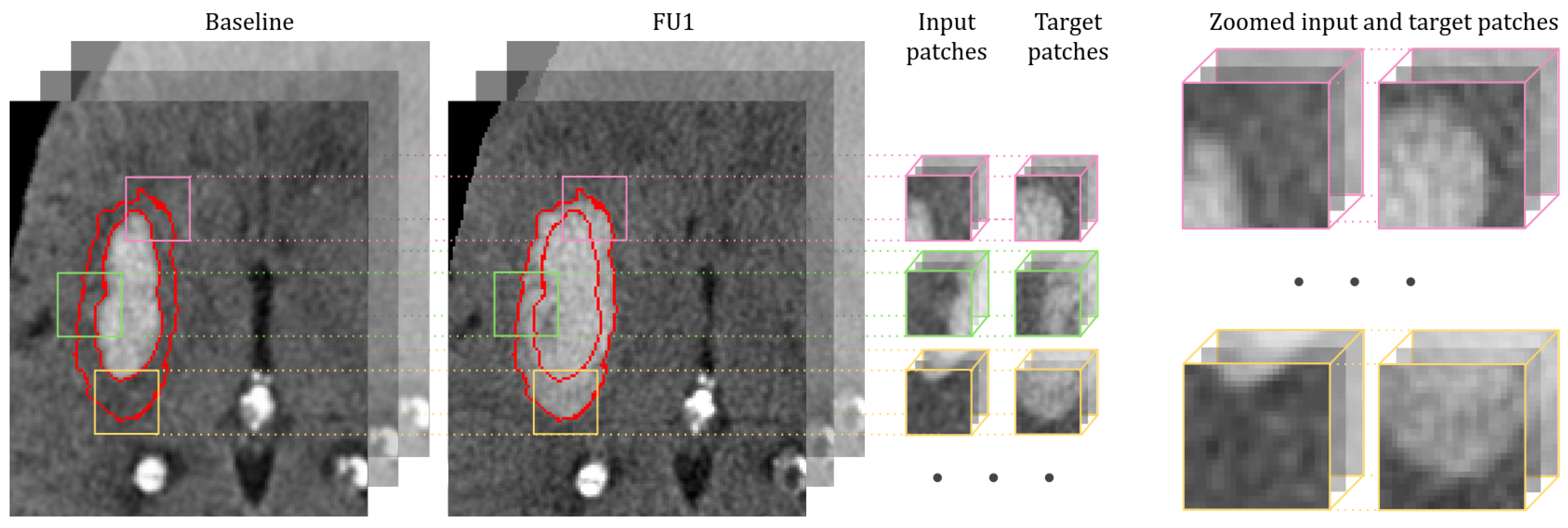
In this work, we present a patch-based CNN algorithm able to predict the final appearance of an expanded hemorrhagic stroke lesion on a brain CT, together with its mask. Our method uses the baseline 3D CT brain image with hemorrhagic stroke and the corresponding hematoma mask as input and outputs the predicted follow-up CT volume and the mask of the resulting lesion. During the training stage, our method learns the possible patterns of HE from the provided training set of real and synthetic images.

2.3. Patch Sampling

The proposed patch-based approach helps us to avoid severe modifications in input images (e.g., down-sampling and resizing), like in the original work of [14], which can significantly distort original images and lead to probable information loss. Nevertheless, the use of patch-based methods also has some issues to consider, e.g., they can suffer from class imbalance, resulting in models biased towards one class over another. Therefore, the process of patch extraction should be controlled and guided with some predefined set of rules. To achieve this, we used a modification of a balanced sampling strategy, where an equal number of patches indicating both classes (lesion and the rest of the brain) is usually extracted from each image. In our case, as we are specifically interested in HE prediction, we want to put more emphasis on the lesion expansion area; therefore, we increase the representation of this class up to 80% of all extracted samples. We define this hematoma growth area as the subtraction between follow-up and baseline lesion masks. This process is illustrated in Figure 2. In addition, we limit the non-lesion patch sampling within the brain mask, to avoid extracting patches from the image background, which does not support any valuable information for the network. In our experiments, we used patches of size 64 × 64 × 64 , as a compromise between the ability of the input sample to fit into memory and the useful content of the patch, preserving more information about the lesion and the growth location together with its shape and size. Moreover, the selected patch size covers the full growth area in most of the cases.

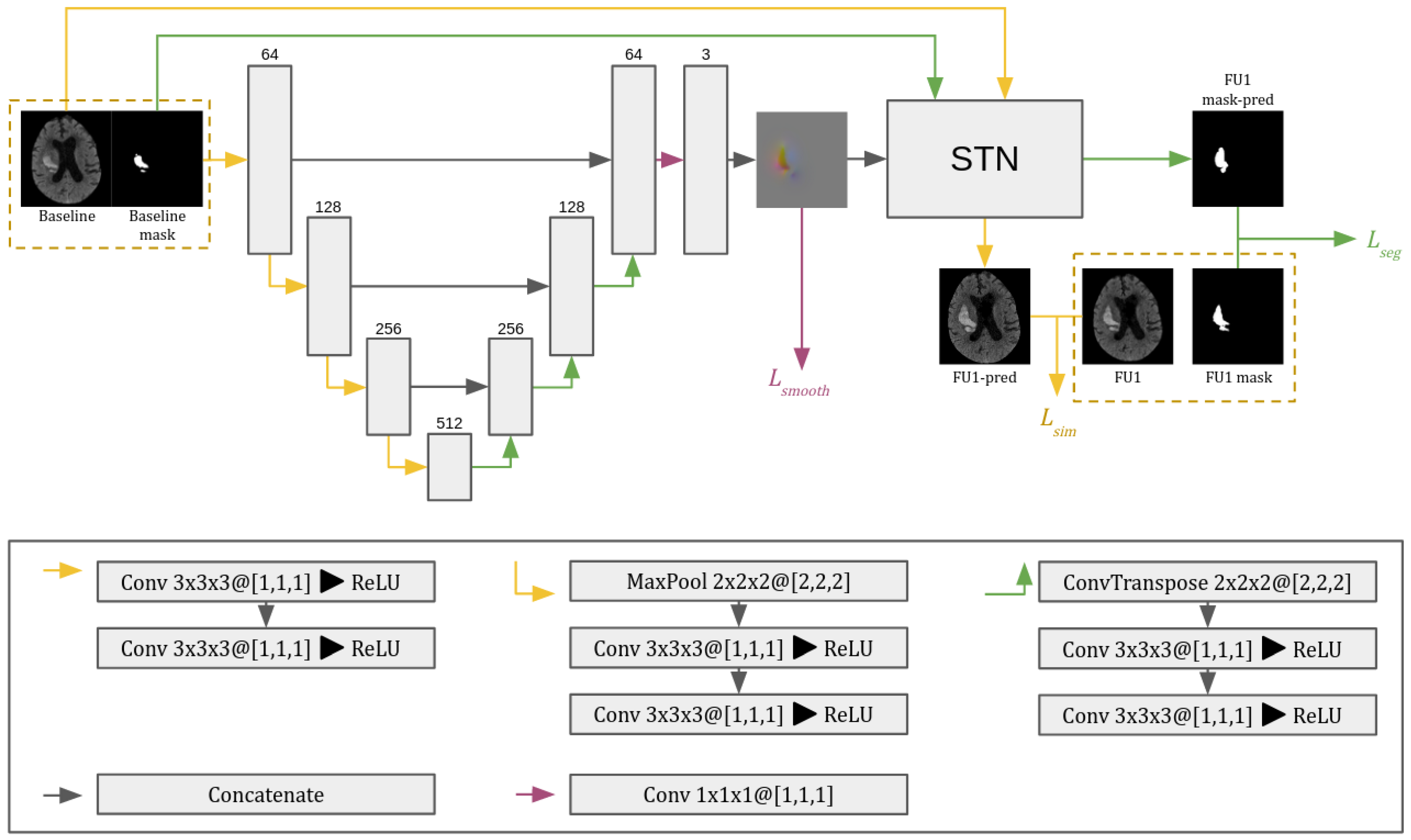
2.4. Network Architecture

As shown in Figure 3, our proposal is based on a 3D U-Net architecture similar to the one of [14]. Each block in the encoding path contains two 3 × 3 × 3 convolutions followed by ReLU. Down-sampling in each resolution step is performed by a 2 × 2 × 2 max pooling operation with a stride of 2. In the decoder, up-sampling is performed with an up-convolution operation of 2 × 2 × 2 with a stride of 2, followed by two 3 × 3 × 3 convolution operations each followed by ReLU. Skip connections are also introduced at each level of the network and allow the decoder to access the higher-resolution features learned by the encoder. We obtain the DVF with a three-channel 1 × 1 × 1 convolution operation without activation function. Then, the spatial transformer network (STN) applies the learned DVF to warp the baseline CT image and its hematoma mask into the predicted follow-up (FU1) CT image and its predicted hematoma mask. The total number of parameters of the proposed network is 22.4 M. The overall configuration of network training and testing is described in the following section.

2.4.1. Training and Testing Processes

The proposed pipeline is trained end to end by using the patches from the baseline brain CT image and its corresponding mask as input, targeting the follow-up brain image and its mask. The DVF output of the U-Net architecture has 3 channels and is of the same spatial size as the input patches. Subsequently, the STN applies this DVF to warp the input image with the mask to the predicted image and its mask. To train this patch-based method, we firstly split the provided cases from the training dataset into training and validation subsets in a ratio of 80% to 20%, respectively. Then, we construct the dataset of patches for both training and validation, where from each image of the corresponding set, we extract 500 patches by following the sampling strategy defined before. Notice that this procedure is performed at the image level, hence avoiding data leakage in training, validation, and testing phases. The model is trained with the Adam optimizer [29], with the learning rate of 0.0001 and batch size of 8. The maximum number of training epochs is 150, with the early stopping of 10 epochs applied. The overall loss function is computed following the same logic as in [14]: L = L seg + L sim + L smooth , where L seg , L sim , and L smooth are individual losses for each part of the pipeline. L seg is the hematoma mask loss, which, in our case, is the Dice loss between the predicted hematoma mask (FU1 mask-pred) and the ground-truth follow-up mask (FU1 mask) (Figure 3, loss shown in green). L sim is the image similarity loss, which is the L 1 between the predicted follow-up image (FU1-pred) and ground-truth follow-up image (FU1) (Figure 3, loss shown in yellow). These two losses are used to learn the DVF, and minimizing them encourages the predicted image and hematoma mask to be similar to their corresponding ground truth. Finally, L smooth (Figure 3, loss shown in magenta) is used to minimize the discrepancy between the transformed image and the target image, i.e., it penalizes the predicted DVF being too complex or noisy, hence helping to avoid producing unrealistic artifacts on the output images. It is a L2 norm regularization term applied to the spatial gradient of the DVF.

2.4.2. Implementation Details

The proposed approach was implemented in Python 3.7 using the Pytorch machine learning framework [30]. All experiments were run on Ubuntu with 256 GB RAM, and network training was performed on a TITAN V GPU with 12 GB of memory.

3. Experimental Results

We carried out three experiments to (1) evaluate the performance of the model in the HE prediction task, (2) demonstrate the influence of adding synthetic images to the training set, and (3) analyze the use of standard data augmentation techniques (i.e., rotation and flipping) on HE pattern prediction. In the baseline experiment, we trained the proposed network with all the steps and characteristics defined in Section 2.4.1 by using the original dataset, without the addition of synthetic images, and disabling the data augmentation performed during training. Then, we performed two more experiments, one extending the baseline experiment with traditional data augmentation and one adding the synthetic images into the training set.
Three metrics were used to evaluate the performance of our predicted volumes: Dice similarity coefficient computed on the expanded area, average prediction error in hematoma volume (AEV), and absolute average error in hematoma volume (AAEV). To evaluate the statistical significance of the obtained results, we used the dependent t-test for paired samples.
Due to the limited number of cases present in the dataset, we performed our experiments using a leave-one-out cross-validation strategy, meaning that every time, only one image was used for testing, while the remaining ones were used for the training and validation of the model. Notice that the proposed synthetic images were only included in the training set, and they were not used for testing. Thus, considering that we had 27 image pairs in our dataset, all the reported results shown in Table 1 are the average of the 27 performed experiments.
Table 1 shows the average metrics obtained with the leave-one-out cross-validation when using only original images, original images with traditional data augmentation, and original images together with the synthetic ones. Note that in general, all the approaches effectively predicted HE with an average Dice score of growth area higher than 0.45 . Further notice that even though the value might seem low, it is relevant, since in most of the cases, the increase was an area of small width compared with the global hematoma volume. From Table 1, we can see that the results of the model using only the original images provided the smallest Dice score, with a clear tendency to undersegment, i.e., generating less growth than expected. This is represented by the negative sign of the AEV value. Notice that this model also produced the highest AAEV, meaning that it was less accurate in predicting the final lesion volume. Additionally, it can be seen that in general, both data augmentation strategies were helpful for improving the obtained results, as expected in situations of scarce training data. The best results in terms of Dice score were obtained with the model that included the synthetic images in training, leading to better prediction of the area of HE and resulting in a nearly 5 % Dice improvement with respect to the model trained only on the original data, with this being statistically significant ( p < 0.05 ), as well as producing a significantly smaller average prediction error in the final lesion volume ( p < 0.05 ). We also computed the Dice score of the total hematoma lesion segmentation with respect to the ground truth of the follow-up images, obtaining similar values for the three models ( 0.757 , 0.763 , and 0.761 , respectively). When comparing our obtained results with the state-of-the-art approach presented in [14], we observed that our quantitative values are in a similar range, providing slightly better performance. For instance, our best mean Dice score of HE was 0.503 vs. 0.467 presented in [14]; we also obtained smaller AEV and AAEV and a global lesion Dice score of 0.763 (vs. 0.735 ). However, we want to emphasize that our dataset is much smaller than the one used in [14], which directly affects this quantitative comparison. Nevertheless, we could achieve similar and sometimes better measures when using synthetic image generation and without requiring the inclusion of patient clinical data.
In Figure 4a, we show the violin plots regarding the distribution of the Dice scores of the HE area for the different studied approaches. We can observe that the median Dice score of the growth area for the setting where we added synthetic images in the training phase is better than the ones of models trained only on original images and using traditional data augmentation. The same behavior can be seen for the interquartile range, which lies between higher values for the model exploiting the use of synthetic images. Furthermore, we noticed that for this setting, the distribution of the Dice scores of the HE area is more concentrated within the median value or higher, which also highlights the use of synthetic images. These results, together with the quantitative measures provided in Table 1, confirm that the addition of the synthetic data generated to improve the training process helps the model to learn HE more precisely, improving the predictions in most of the cases. Figure 4b shows the distribution of the prediction error in hematoma volume obtained with the proposed models. Again, we can see that both traditional data augmentation and image synthesis approaches reduce the error in the predicted volume, moving the median of the errors towards zero. Moreover, the distribution of the AEV obtained with the model trained using synthetic images has smaller interquartile ranges than the other two models, producing more robust and consistent results.
A qualitative comparison among the different models is illustrated in Figure 5, where we show several examples with the baseline and follow-up CT images and the corresponding ground-truth masks, together with the predicted FU1 images and segmentation masks obtained with the three different models evaluated. The colors of the overlayed masks represent true-positive voxels, which are shown in red, false-positive voxels in green, and false-negative voxels in blue. From Figure 5a,b we see that the model trained with the addition of synthetic images better predicts the resulting hematoma masks, producing less false positives and false negatives. Regarding the example shown in Figure 5c, we see that the model trained with the incorporation of synthetic images better perceives the pattern of growth of such elongated lesions, producing more growth along the longitudinal axis of the initial stroke lesion. From Figure 5d, we can see that none of the three models were able to predict the lesion growth perfectly, but in this particular case, the initial lesion presented quite an irregular shape. Of note, the predicted masks of the models trained on original images only and with traditional data augmentation techniques contain a vast number of false-positive voxels, and visually, they appear uniformly spread around the ground truth, which suggest that these models mostly learn to produce somewhat uniform growth, while extending the training dataset with synthetic images helps the model to be more accurate in learning the possible HE patterns.
To analyze the performance of our models in the best possible scenario, our approach relies on the spatial constraint provided by the ground truth of the hematoma mask in the initial CT scan. Therefore, the model does not have a bias due to the errors produced by the automated segmentation approach. Nevertheless, the current state-of-the-art approaches for hematoma segmentation [24,31] achieve more than 0.85 in Dice score, making a good starting point for the prediction pipeline. To validate this, we performed an experiment where the leave-one-out cross-validation strategy was applied directly by using the automated segmentation mask provided by the segmentation approach [24]. The obtained results provided a Dice score of growth of 0.472 ± 0.134 versus the 0.506 ± 0.120 obtained when using the ground-truth masks. As expected, we noticed a slight drop in Dice score, but these results are still in line with our main findings and the ones of the state-of-the-art approach (Dice score of growth 0.467), proving that the initialization of the mask was already good enough not to affect the prediction results.

4. Discussion

In this study, we have presented a patch-based deep learning approach for predicting the hemorrhagic stroke lesion area after its expansion. This problem is very challenging, considering that there is still no full understanding of the mechanisms and patterns of HE and that there are no publicly available large datasets with their corresponding annotations. Our proposal requires only CT imaging data with lesion annotations for training the models. We addressed the challenge of having limited annotated data of HE to perform the training of the models. To overcome this issue, we adapted the image synthesis proposed in [23] to generate more longitudinal training samples for hemorrhagic stroke lesions. This is a fully customizable and straightforward approach which does not require preliminary training. We analyzed the performance of different models: (1) training only on the original CT images, (2) training on the original images and the usage of standard data augmentation techniques, and (3) training on the original images with the addition of the generated synthetic images. All these models achieved results similar to those reported in the only related work available on the state of the art [14] but were obtained by using fewer data and without the need of adding non-imaging data. We observed that the model trained with the inclusion of the synthetic images produced overall better predictions of HE areas compared with the other analyzed models and the current results of the work of [14]. Notice that our deep learning approach is patch-based, meaning that we do not need to alter the original images; hence, we avoid losing important information regarding the hematoma growth pattern. Overall, with the leave-one-out evaluation performed, we obtained a mean Dice score for the growth area of 0.503 , which is in line with the Dice score provided in the work of [14] (mean of 0.467 ). By analyzing the results per patient, we observed that the inclusion of image synthesis in the training process allowed us to improve the performance, obtaining higher Dice scores in 19 out of the 27 analyzed patients (this can be seen in Figure 4a), which was statistically significant with respect to the model trained only on original images ( p < 0.05 ). Furthermore, the model using the synthetic images could significantly reduce the average prediction error in hematoma volume ( p < 0.05 ), helping the model to be more robust and consistent in its predictions.
In all our experiments, we observed overall an undersegmentation trend, as can be seen in the examples of Figure 5. This mostly happens in cases that have lesions with a high initial volume and a real growth value of more than 50%. Typically, the worst prediction results were obtained in cases with lesions that presented smaller average growth areas; therefore, small prediction errors directly affected the Dice score computation. From the obtained results, we observed that the incorporation of synthetic images was beneficial in cases with lesions of irregular shape or with irregular HE patterns. Even though their metrics may be lower than for more uniform lesions overall, the results were improved with the addition of synthetic data mainly due to the fact that we increased the representation of different lesions and HE growth patterns within the training dataset by doing so. Moreover, we observed that our approach tended to produce better predictions in cases with more uniformly shaped lesions, where augmenting the dataset using traditional data augmentation techniques or using the generated synthetic images helped to obtain better and more robust results.
This study also has some limitations. The main one is the size of the available dataset that was used to train and evaluate our approaches. Our proposed model would indeed benefit from having more HE cases for the training process and also from having an independent testing dataset. However, in clinical practice, it is hard to collect a large number of cases with HE condition, having also the corresponding annotations. Moreover, to the best of our knowledge, there are currently no publicly available datasets with longitudinal CT images of HE cases. Nevertheless, this study shows that even in a situation presenting a scarcity of data, the proposed approach, together with the inclusion of synthetic images, allows promising results to be obtained. In future work, we plan to extend this study with a bigger multicentric dataset, which could help both to obtain better models and to perform external independent validation, analyzing the model capability to generalize its application to different datasets and scanners. Another point for future work would be to incorporate relevant clinical data into the developed model to test its influence on the final results.

5. Conclusions

In this work, we proposed a deep learning method for predicting HE from brain CT images. This is a challenging task that, to the best of our knowledge, is still under-explored in the literature. Our approach is based only on imaging data and uses a 3D patch-based U-Net architecture to learn the deformation of hematoma between two timepoints and obtain a prediction of the HE area in a patient from the initial CT image. We also tackled the problem of having a limited dataset, studying the impact of using traditional data augmentation techniques and the addition of synthetic images to improve model performance. Our findings from the experimental tests showed that our method achieved satisfactory results in predicting the HE area with an average Dice score of the expanded area of 0.506 and an average inference time of 50 s per patient. From a clinical point of view, such a tool could complement the work of clinicians in order to predict the probable extent of hemorrhagic stroke at the time of the initial patient CT scan, helping to perform a better stratification of patients with higher risk of high-grade HE, thus optimizing individual treatment decisions. The code of this project is available at https://github.com/NIC-VICOROB/hematoma-expansion-prediction.git.

Author Contributions

Conceptualization, V.A., A.O. and X.L.; methodology, V.A., A.O., M.T., Y.S. and X.L.; software, V.A.; validation, M.T. and Y.S.; formal analysis, A.O., J.S. and X.L.; investigation, V.A.; resources, M.T. and Y.S.; writing—original draft preparation, V.A.; writing—review and editing, A.O., J.S. and X.L.; supervision, A.O., J.S. and X.L. All authors have read and agreed to the published version of the manuscript.

Funding

Valeriia Abramova received an FPI grant from Ministerio de Ciencia, Innovación y Universidades with reference number PRE2021-099121. This work was supported under DPI2020-114769RB-I00 from Ministerio de Ciencia, Innovación y Universidades and also by the ICREA Academia program.

Institutional Review Board Statement

The study was conducted in accordance with the Declaration of Helsinki, and approved by the Ethics Committee of Josep Trueta University Hospital (protocol code 284/U/2017).

Informed Consent Statement

Not applicable.

Data Availability Statement

The dataset provided in this article is not available due to regulations of the collaborating hospital.

Acknowledgments

The authors gratefully acknowledge the support of NVIDIA Corporation through their donation of the GPU used in this research.

Conflicts of Interest

The authors declare no conflicts of interest.

References

  1. Feigin, V.L.; Stark, B.A.; Johnson, C.O.; Roth, G.A.; Bisignano, C.; Abady, G.G.; Abbasifard, M.; Abbasi-Kangevari, M.; Abd-Allah, F.; Abedi, V.; et al. Global, regional, and national burden of stroke and its risk factors, 1990–2019: A systematic analysis for the Global Burden of Disease Study 2019. Lancet Neurol. 2021, 20, 795–820. [Google Scholar] [CrossRef] [PubMed]
  2. Norrving, B.; Kissela, B. The global burden of stroke and need for a continuum of care. Neurology 2013, 80, S5–S12. [Google Scholar] [CrossRef]
  3. Yang, W.S.; Zhang, S.Q.; Shen, Y.Q.; Wei, X.; Zhao, L.B.; Xie, X.F.; Deng, L.; Li, X.H.; Lv, X.N.; Lv, F.J.; et al. Noncontrast Computed Tomography Markers as Predictors of Revised Hematoma Expansion in Acute Intracerebral Hemorrhage. J. Am. Heart Assoc. 2021, 10, e018248. [Google Scholar] [CrossRef]
  4. Brott, T.; Broderick, J.; Kothari, R.; Barsan, W.; Tomsick, T.; Sauerbeck, L.; Spilker, J.; Duldner, J.; Khoury, J. Early Hemorrhage Growth in Patients with Intracerebral Hemorrhage. Stroke 1997, 28, 1–5. [Google Scholar] [CrossRef] [PubMed]
  5. Haupenthal, D.; Schwab, S.; Kuramatsu, J.B. Hematoma expansion in intracerebral hemorrhage—The right target? Neurol. Res. Pract. 2023, 5, 36. [Google Scholar] [CrossRef]
  6. Heit, J.J.; Iv, M.; Wintermarkl, M. Imaging of Intracranial Hemorrhage. J. Stroke 2017, 19, 11–27. [Google Scholar] [CrossRef] [PubMed]
  7. Demchuk, A.M.; Dowlatshahi, D.; Rodriguez-Luna, D.; Molina, C.A.; Blas, Y.S.; Dzialowski, I.; Kobayashi, A.; Boulanger, J.M.; Lum, C.; Gubitz, G.; et al. Prediction of haematoma growth and outcome in patients with intracerebral haemorrhage using the CT-angiography spot sign (PREDICT): A prospective observational study. Lancet Neurol. 2012, 11, 307–314. [Google Scholar] [CrossRef]
  8. Nehme, A.; Ducroux, C.; Panzini, M.A.; Bard, C.; Bereznyakova, O.; Boisseau, W.; Deschaintre, Y.; Diestro, J.D.B.; Guilbert, F.; Jacquin, G.; et al. Non-contrast CT markers of intracerebral hematoma expansion: A reliability study. Eur. Radiol. 2022, 32, 6126–6135. [Google Scholar] [CrossRef]
  9. Morotti, A.; Boulouis, G.; Dowlatshahi, D.; Li, Q.; Shamy, M.; Salman, R.A.S.; Ros, J.; Cordonnier, C.; Goldstein, J.N.; Charidimou, A. Intracerebral haemorrhage expansion: Definitions, predictors, and prevention. Lancet Neurol. 2023, 22, 159–171. [Google Scholar] [CrossRef]
  10. Morotti, A.; Boulouis, G.; Dowlatshahi, D.; Li, Q.; Barras, C.D.; Delcourt, C.; Yu, Z.; Zheng, J.; Zhou, Z.; Aviv, R.I.; et al. Standards for Detecting, Interpreting, and Reporting Noncontrast Computed Tomographic Markers of Intracerebral Hemorrhage Expansion. Ann. Neurol. 2019, 86, 480–492. [Google Scholar] [CrossRef]
  11. Greenberg, S.M.; Ziai, W.C.; Cordonnier, C.; Dowlatshahi, D.; Francis, B.; Goldstein, J.N.; Hemphill, J.C.; Johnson, R.; Keigher, K.M.; Mack, W.J.; et al. Guideline for the Management of Patients with Spontaneous Intracerebral Hemorrhage: A Guideline from the American Heart Association/American Stroke Association. Stroke 2022, 53, e282–e361. [Google Scholar] [CrossRef] [PubMed]
  12. Samak, Z.A.; Clatworthy, P.; Mirmehdi, M. FeMA: Feature matching auto-encoder for predicting ischaemic stroke evolution and treatment outcome. Comput. Med. Imaging Graph. 2022, 99, 102089. [Google Scholar] [CrossRef] [PubMed]
  13. Wouters, A.; Robben, D.; Christensen, S.; Marquering, H.A.; Roos, Y.B.; van Oostenbrugge, R.J.; van Zwam, W.H.; Dippel, D.W.; Majoie, C.B.; Schonewille, W.J.; et al. Prediction of Stroke Infarct Growth Rates by Baseline Perfusion Imaging. Stroke 2022, 53, 569–577. [Google Scholar] [CrossRef] [PubMed]
  14. Xiao, T.; Zheng, H.; Wang, X.; Chen, X.; Chang, J.; Yao, J.; Shang, H.; Liu, P. Intracerebral Haemorrhage Growth Prediction Based on Displacement Vector Field and Clinical Metadata. In Proceedings of the Medical Image Computing and Computer Assisted Intervention—MICCAI 2021, Strasbourg, France, 27 September–1 October 2021; Springer International Publishing: Berlin/Heidelberg, Germany, 2021; pp. 741–751. [Google Scholar] [CrossRef]
  15. Song, Z.; Guo, D.; Tang, Z.; Liu, H.; Li, X.; Luo, S.; Yao, X.; Song, W.; Song, J.; Zhou, Z. Noncontrast Computed Tomography-Based Radiomics Analysis in Discriminating Early Hematoma Expansion after Spontaneous Intracerebral Hemorrhage. Korean J. Radiol. 2021, 22, 415. [Google Scholar] [CrossRef] [PubMed]
  16. Al Khalil, Y.; Amirrajab, S.; Lorenz, C.; Weese, J.; Pluim, J.; Breeuwer, M. On the usability of synthetic data for improving the robustness of deep learning-based segmentation of cardiac magnetic resonance images. Med. Image Anal. 2023, 84, 102688. [Google Scholar] [CrossRef] [PubMed]
  17. Xu, Z.; Tang, J.; Qi, C.; Yao, D.; Liu, C.; Zhan, Y.; Lukasiewicz, T. Cross-domain attention-guided generative data augmentation for medical image analysis with limited data. Comput. Biol. Med. 2024, 168, 107744. [Google Scholar] [CrossRef] [PubMed]
  18. Zhang, Z.; Yang, L.; Zheng, Y. Translating and Segmenting Multimodal Medical Volumes with Cycle- and Shape-Consistency Generative Adversarial Network. In Proceedings of the IEEE Conference on Computer Vision and Pattern Recognition (CVPR), Salt Lake City, UT, USA, 18–23 June 2018; pp. 9242–9251. [Google Scholar]
  19. Zhang, Z.; Deng, H.; Li, X. Unsupervised Liver Tumor Segmentation with Pseudo Anomaly Synthesis. In Proceedings of the SASHIMI 2023: Simulation and Synthesis in Medical Imaging, Vancouver, BC, Canada, 8 October 2023; Lecture Notes in Computer Science. Springer Nature Switzerland: Cham, Switzerland, 2023; pp. 86–96. [Google Scholar] [CrossRef]
  20. Basaran, B.D.; Qiao, M.; Matthews, P.M.; Bai, W. Subject-Specific Lesion Generation and Pseudo-Healthy Synthesis for Multiple Sclerosis Brain Images. In Proceedings of the SASHIMI 2022: Simulation and Synthesis in Medical Imaging, Singapore, 18 September 2022; Lecture Notes in Computer Science. Springer International Publishing: Cham, Switzerland, 2022; pp. 1–11. [Google Scholar] [CrossRef]
  21. Wang, Y.; Ji, Y.; Xiao, H. A data augmentation method for fully automatic brain tumor segmentation. Comput. Biol. Med. 2022, 149, 106039. [Google Scholar] [CrossRef] [PubMed]
  22. Bernal, J.; Valverde, S.; Kushibar, K.; Cabezas, M.; Oliver, A.; Lladó, X. Generating Longitudinal Atrophy Evaluation Datasets on Brain Magnetic Resonance Images Using Convolutional Neural Networks and Segmentation Priors. Neuroinformatics 2021, 19, 477–492. [Google Scholar] [CrossRef]
  23. Larson, K.E.; Oguz, I. Synthetic Atrophy for Longitudinal Cortical Surface Analyses. Front. Neuroimaging 2022, 1, 861687. [Google Scholar] [CrossRef]
  24. Abramova, V.; Abramova, V.; Clerigues, A.; Quiles, A.; Figueredo, D.G.; Silva, Y.; Pedraza, S.; Oliver, A.; Lladó, X. Hemorrhagic stroke lesion segmentation using a 3D U-Net with squeeze-and-excitation blocks. Comput. Med. Imaging Graph. 2021, 90, 101908. [Google Scholar] [CrossRef]
  25. Beare, R.; Lowekamp, B.; Yaniv, Z. Image Segmentation, Registration and Characterization in R with SimpleITK. J. Stat. Softw. 2018, 86, 1–35. [Google Scholar] [CrossRef] [PubMed]
  26. Yaniv, Z.; Lowekamp, B.C.; Johnson, H.J.; Beare, R. SimpleITK Image-Analysis Notebooks: A Collaborative Environment for Education and Reproducible Research. J. Digit. Imaging 2017, 31, 290–303. [Google Scholar] [CrossRef] [PubMed]
  27. Lowekamp, B.C.; Chen, D.T.; Ibáñez, L.; Blezek, D. The Design of SimpleITK. Front. Neuroinform. 2013, 7, 45. [Google Scholar] [CrossRef] [PubMed]
  28. Yushkevich, P.A.; Pluta, J.; Wang, H.; Wisse, L.E.; Das, S.; Wolk, D. IC-P-174: Fast Automatic Segmentation of Hippocampal Subfields and Medial Temporal Lobe Subregions In 3 Tesla and 7 Tesla T2-Weighted MRI. Alzheimer’s Dement. 2016, 12, 126–127. [Google Scholar] [CrossRef]
  29. Kingma, D.P.; Ba, J. Adam: A Method for Stochastic Optimization. arXiv 2014. [Google Scholar] [CrossRef]
  30. Paszke, A.; Gross, S.; Chintala, S.; Chanan, G.; Yang, E.; De Vito, Z.; Lin, Z.; Desmaison, A.; Antiga, L.; Lerer, A. Automatic differentiation in PyTorch. In Proceedings of the NIPS-W, Long Beach, CA, USA, 4–9 December 2017; pp. 1–4. [Google Scholar]
  31. Kuang, Z.; Deng, X.; Yu, L.; Wang, H.; Li, T.; Wang, S. Ψ-Net: Focusing on the border areas of intracerebral hemorrhage on CT images. Comput. Methods Programs Biomed. 2020, 194, 105546. [Google Scholar] [CrossRef]
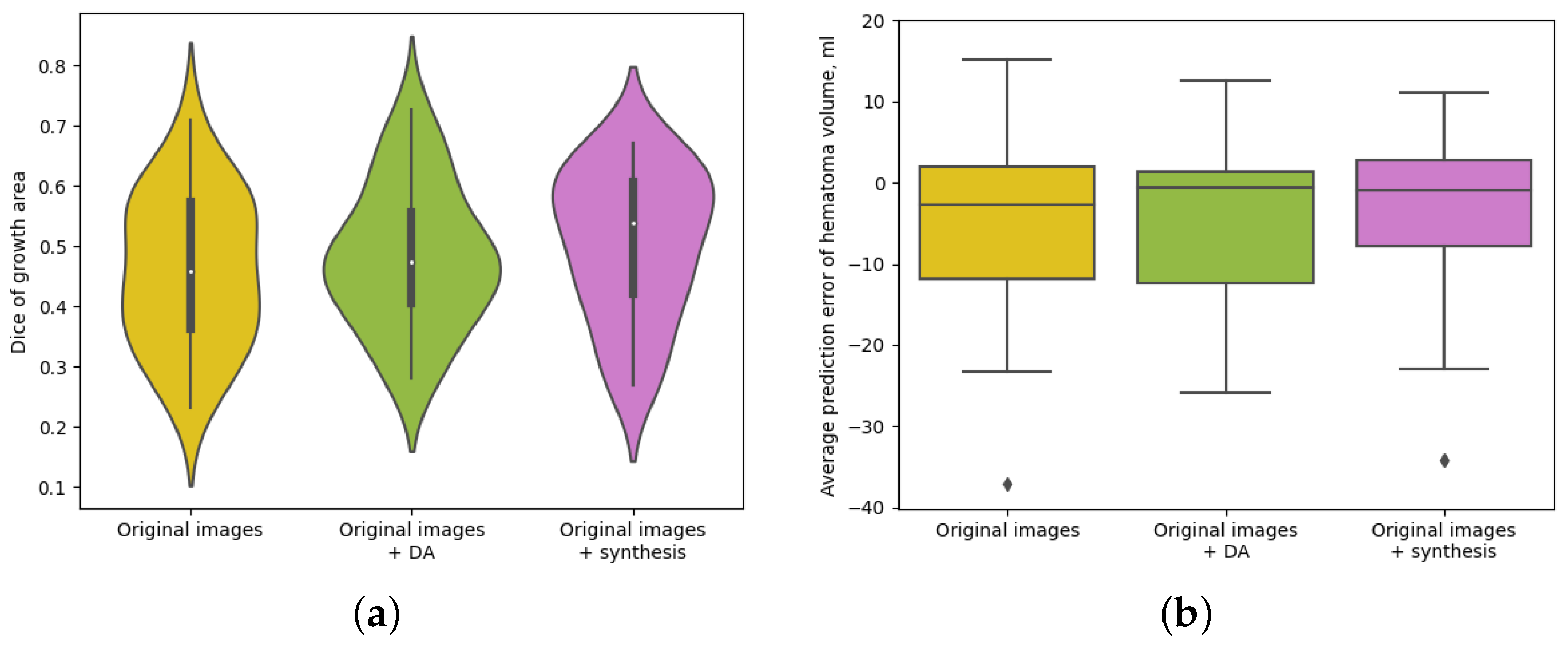
Figure 1. Schematic process of image generation with synthetically induced lesion deformation. (A) Original baseline lesion mask. (B) The target lesion mask (shown in white) obtained after a binary erosion operation on the original lesion mask (shown in gray). (C) Deformation field produced after registration of the original mask to the target lesion mask. Different colors of the image represent values and directions of all 3D vectors of the DVF. (D) Original baseline CT image. (E) The resulting CT image obtained after applying the deformation field to the original CT image.
Applsci 14 02708 g001
Figure 2. Illustration of the patch sampling process during training within the lesion expansion area. The procedure is shown for the input CT image and the target follow-up CT image, and the same applies for the input baseline hematoma mask and the target follow-up hematoma mask. Of all patches, 80 % are sampled from the HE area, meaning that the center of the patch is located within this region (marked with red contours). The input and target patches are extracted from the same location of the baseline and follow-up CT images (masks). The colors of the patch borders mark each training pair. Zoomed input and target patches show that we are aiming to learn information from the hematoma growth area.
Applsci 14 02708 g002
Figure 3. The 3D CNN architecture used in the proposed approach. The network consists of a 3D U-Net with skip connections and a spatial transformer network (STN). In the convolutional layers (Conv), KxKyKz@[Sx,Sy,Sz] indicates the kernel and stride dimensions in each axis. The gray boxes represent the feature maps, with the number of channels indicated above them. L seg is the segmentation loss computed between output and target masks; L sim is the similarity loss between output and target images; and L smooth restricts unrealistic displacement changes.
Applsci 14 02708 g003
Figure 4. Dice scores and hematoma volume prediction for the three different analyzed models. DA stands for traditional data augmentation. (a) Violin plots showing the distribution of Dice scores computed for the expansion area for different methods. (b) Boxplots showing the distribution of the prediction error in total hematoma volume for different methods.
Applsci 14 02708 g004
Figure 5. Examples of the resulting masks obtained in our experiments. For each case (ad), the top row shows (from left to right): baseline CT image, follow-up CT image, follow-up CT image overlayed with the resulting mask from the experiment performed only with original images, follow-up CT image overlayed with the resulting mask from the experiment performed with original images and traditional data augmentation, and follow-up CT image overlayed with the resulting mask from the experiment performed with original and synthetic images. The colors of the overlayed masks represent true-positive voxels (red), false-positive voxels (green), and false-negative voxels (blue). The bottom row for each case (ad) shows the corresponding hematoma masks. DA stands for traditional data augmentation.
Applsci 14 02708 g005
Table 1. The average metrics across 27 leave-one-out experiments compared with the results of [14]. DA stands for traditional data augmentation. The values in bold specify the highest metric value. The significance of adding synthetic images to the training set is shown with * (*—significant at p < 0.05 ).
Dice of Growth (↑)AEV, mL (↔)AAEV, mL (↓)
Original images0.458 ± 0.125 5.81 ± 11.54 9.20 ± 8.96
Original images + DA0.481 ± 0.118 5.09 ± 10.12 8.15 ± 7.77
Original images + synthesis0.506 ± 0.120 * 3.44 ± 11.87 *8.49 ± 8.85
Xiao et al. [14]0.4674.8010.50
* Significant at p < 0.05 .
Disclaimer/Publisher’s Note: The statements, opinions and data contained in all publications are solely those of the individual author(s) and contributor(s) and not of MDPI and/or the editor(s). MDPI and/or the editor(s) disclaim responsibility for any injury to people or property resulting from any ideas, methods, instructions or products referred to in the content.

