Environmental Interference Suppression by Hybrid Segmentation Algorithm for Open-Area Electromagnetic Capability Testing

Abstract

Compared with electromagnetic compatibility (EMC) testing in anechoic rooms, open-area EMC testing takes advantage of in situ and engine running status measurement but suffers from non-negligible external electromagnetic interference. This paper proposes a novel environmental interference suppression method (named the EMC environmental interference suppression algorithm ($E^{2}ISA$)) that separates signals from backgrounds via image segmentation and recognizes the near–far site signal via a group of time-varying features based on the difference in the near-site EM radiative characteristic. We find that the proposed $E^{2}ISA$ method, which combines the deep learning segmentation network with the classical recognition methods, is able to suppress environmental interference signals accurately. The experiment results show that the accuracy of $E^{2}ISA$ reaches up to 95% in the face of VHF (Very High Frequency) EMC testing tasks.

1. Introduction

Electromagnetic compatibility (EMC) testing works to ascertain the emissions and susceptibility of equipment, which play a crucial role in the communication, radar, and aerospace fields and the automotive industry. At present, EMC measurements can be implemented in open-area sites [1], screened rooms [2], and anechoic rooms [3]. Among them, the screened room surrounded by all-metal materials can be isolated from external electromagnetic interference to a high degree. Anechoic rooms can improve the measurement performance by lining the walls and ceiling with absorbing materials. Suffering from immovability, neither of them can be applied for in situ measurement or engine running status measurement. Open-area testing takes EMC measurements on a flat metalized ground area, and the observed signal is the superposition of the directly arriving signals and their reflection from the ground. Compared with the screened room and anechoic room testing, open-area testing is more flexible, which is suitable for in situ measurement or engine running status measurement, but it suffers from non-negligible external electromagnetic interference.

From the aspect of signal analysis, external electromagnetic interference can be divided into two kinds, frequency-domain separable interference [4] and frequency-domain nonseparable interference [5]. For the former one, the interference of different equipment has different frequency regions and can be recognized. For the latter one, the interference of different equipment occupies the same frequency region, which makes it difficult to separate. Since most of the man-made interference is with a single-frequency or narrow-frequency occupancy, the frequency-domain separable interference plays a dominant role in open-area EMC testing.

After separating different signals in the frequency domain, segmentation can be applied for further processing, which can generally be divided into two classes, semantic segmentation [6] and instance segmentation [7]. Semantic segmentation labels all image pixels with a set of object categories, and targets in the same category can not be distinguished. Recently, segmentation methods based on deep learning have achieved great progress and have been applied in different fields successfully.

In this paper, an environmental interference suppression method named the EMC environmental interference suppression algorithm ($E^{2}ISA$) is proposed. Firstly, a hybrid segmentation algorithm that combines U-net with a classical connected component analysis algorithm is proposed to separate different signals in the time–frequency domain from the background. Then, a group of feature similarity decision criteria, named SLTVSFs, are designed to reflect the changes in the statistics of each signal with time. Finally, the KL divergence, JS divergence, cosine similarity, and Pearson correlation coefficient are calculated for near–far site recognition.

The organization of this paper is as follows: In Section 2, the system configuration of our open-area EMC testing method is introduced briefly. In Section 3, the EMC environmental interference suppression algorithm is proposed and analyzed in detail. In Section 4, a group of experiments with real data are carried out to verify the performance of the proposed algorithms. A summary is given in Section 5.

2. System Configuration of Open-Area EMC Testing

2.1. Review on EM Radiative Characteristics

In electromagnetic compatibility testing, the signal and interference are transmitted to the measurement antennas in free space, whose radiative characteristics can be divided into three fields: the reactive near field, radiative near field, and far field (radiation zone). The reactive near field is near to 0.159 times the wavelength (referred to as the $\lambda$). Given the allocation of civil aviation bands between 118 MHz and 137 MHz and the operation of the VHF omnidirectional range (VOR) between 108 MHz and 117.95 MHz, we have focused our EMC testing specifically on the VHF band to address aviation equipment EMC issues. Assuming that EMC testing is operated at 100 MHz, the upper bound of the reactive near field is about 0.5 m, which is shorter than the actual distance between the radiant source and measurement antenna (which is always larger than 1 m).

The radiative near field (or Fresnel region) covers the region of the reactive near field to the Fraunhofer distance [8], which is calculated as $2D^2/\lambda$ (where D denotes the aperture of the radiant source). Assuming that $D=0.2 \mathrm{m}$ and $\lambda =3 \mathrm{m}$ (corresponding to 100 MHz), the Fraunhofer distance is about $0.0267 \mathrm{m}$, which indicates that there is no radiative near field for 100 MHz EMC testing (VHF aeronautical telecommunication band). When $\lambda$ = 0.03 m (corresponding to 10 GHz), the Fraunhofer distance is about $2.67$ m, which covers the one-meter EMC testing. In this case, the electric field strength is proportional to the inverse square of the distance, i.e., $1/r^2$.

The radiative far field (radiation zone) covers the region out of the radiative near field, which is the main working zone for VHF band EMC testing. In this case, the electric field strength is proportional to the inverse distance, i.e., $1/r$. If there is a measurement antenna placed 3 m away from the internal radiant source (such as the device under test (DUT)) and another measurement antenna placed 6 m away from the internal radiant source, there is a 6 dB falloff between the near-site antenna and far-site antenna. In contrast, if there is a measurement antenna placed 103 m away from the environmental radiant source and another measurement antenna placed 106 m away from the environmental radiant source, there is only a 0.2494 dB falloff between the near-site antenna and far-site antenna (in this case, we obtain the plane wave approximation). Based on this, we can estimate the distance of radiant sources via the two-antenna method by calculating the near–far amplitude falloff of different signals on the frequency spectrum, which is the principle of this paper.

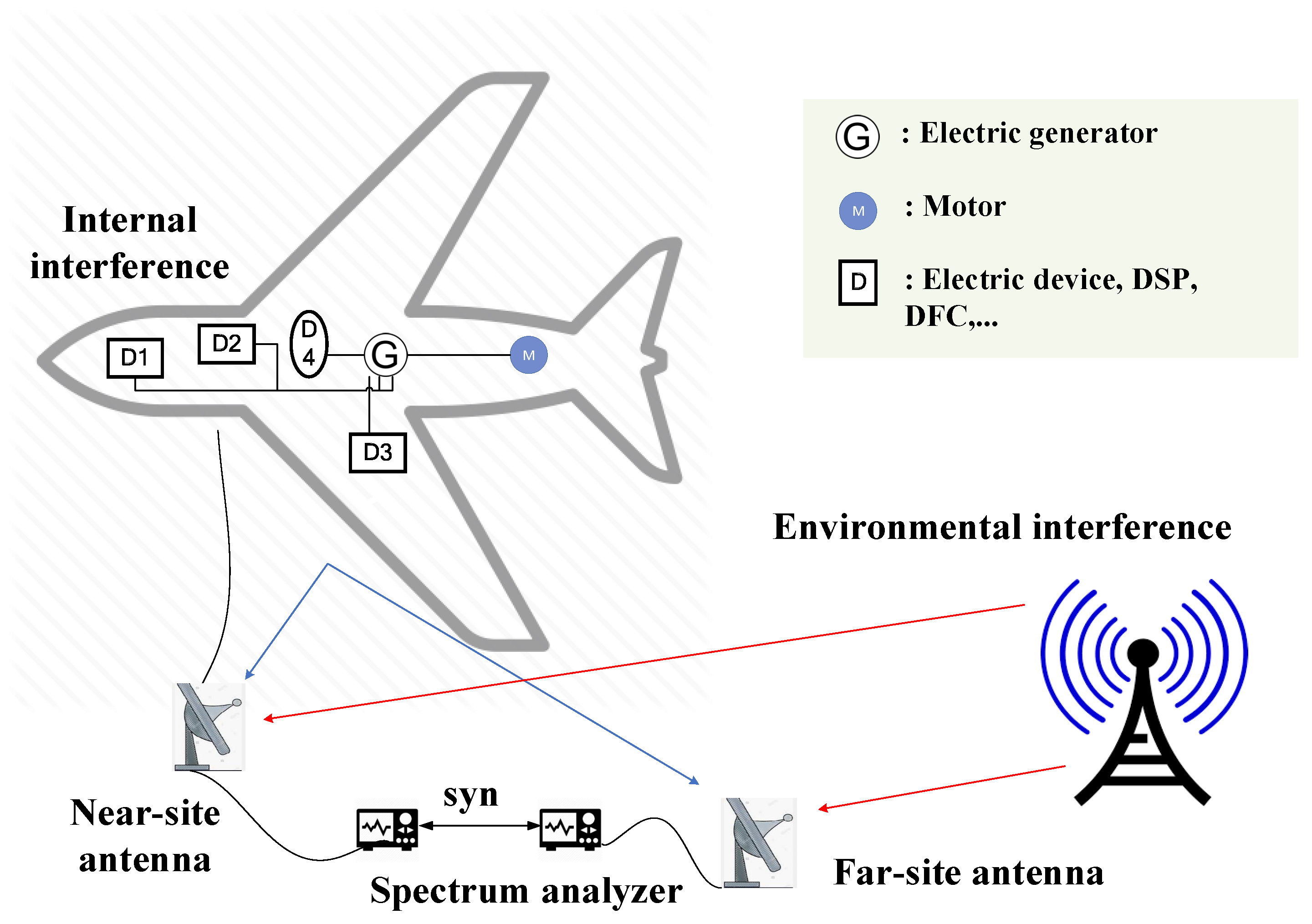
2.2. Near–Far EMC Testing Configuration

Based on the EM radiative characteristic, our open-area EMC testing system is designed by using a near–far EMC testing configuration similar to that used in the literature [9,10], which is shown in Figure 1. The symbols “G”, “M”, and “D” refer to the typical internal interferences of a plane. G denotes the electric generator, M denotes the motor, and D denotes the other electric devices, such as the digital signal processor (DSP) and digital flight controller (DFC).

There are two omnidirectional measurement antennas connected to two spectrum analyzers (SA), which are synchronized by setting one of them as the internal trigger and the other one as the external trigger. One of the measurement antennas (named the near-site antenna) is placed near the radiant source (or device under test (DUT)) ( 1 m or 3 m), and the other one (named the far-site antenna) is placed far away from the radiant source ( 9 m or further).

Then, the waterfall figures of the two spectrum analyzers are captured, which contain both the signal and environmental interference. According to the EM radiative characteristic, when the signal is near the testing site, i.e., the DUT, the received signal falls off significantly with the distance. As a result, the signal strength of the near-site antenna is larger than the far-site antenna. In contrast, when the signals come from far away from the DUT, we consider them to be environmental interference, and the distances to the near-site and far-site antennas are almost the same. As a result, the signal strengths of the near-site and far-site antennas are similar. Based on this feature, the environmental interference can be clearly recognized from the internal signal and easily suppressed.

A shortcoming of the near–far EMC testing configuration is the need to deal with the frequency spectrum superposition problem. In this case, the internal interference occupies the same frequency band as the environmental interference. Thus, the two spectrum analyzers (SAs) acquire the superposition of the internal and environmental interferences. The effect of the frequency spectrum superposition depends on the relative intensities of the internal and environmental interferences. If they possess the same intensity, the superposed intensity will theoretically range from 0 (exact cancellation) to 2 times the original intensity (coherent accumulation).

For independent Gaussian stochastic signals, the variance of the superposed signal is the sum of the variances of the internal and environmental interferences. When the variance of the internal interference is 10 and the variance of the environmental interference is 1, the superposed variance will be 0.41 dB larger than that of the desired one (internal interference), which is acceptable in practice. Conversely, when the variance of the internal interference is 1 and the variance of the environmental interference is 10, the superposed variance will be 10.41 dB larger than that of the desired one (internal interference). In this case, the superposition phenomenon violates the assumption of electromagnetic (EM) radiative characteristics and greatly deteriorates the recognition and suppression of internal and environmental interferences. Thus, the frequency spectrum separability should be examined before employing the near–far EMC open-area testing method.

3. Open-Area Environmental Interference Suppression Model

A deep-learning-based environmental interference suppression method is proposed in this section, named the EMC environmental interference suppression algorithm ($E^{2}ISA$), which can suppress the environmental interferences from the internal signal accurately and efficiently.

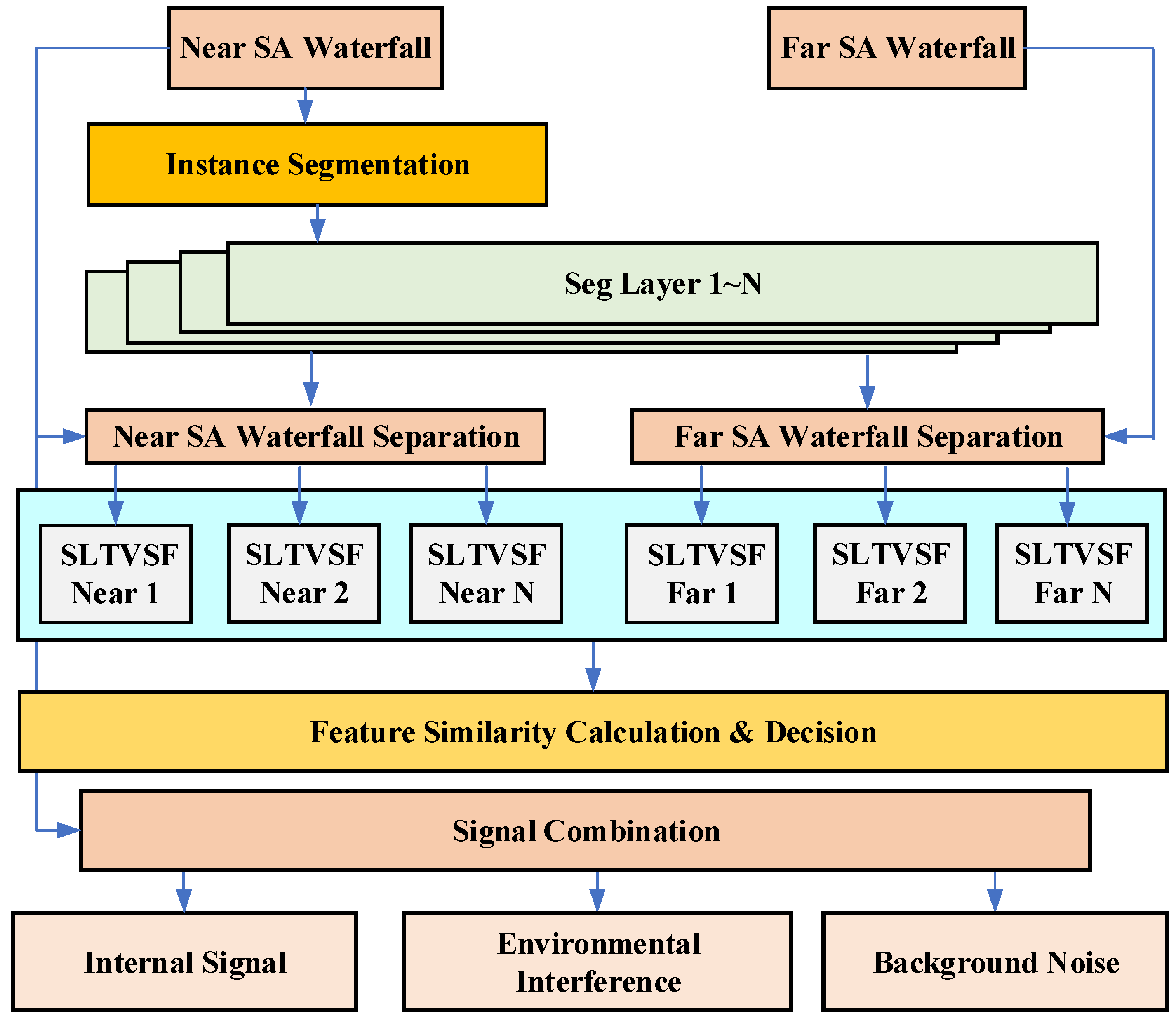
3.1. Environmental Interference Suppression Framework

A diagram of the environmental interference suppression framework is shown in Figure 2. Since the signal strengths of the near SA waterfall are often stronger than and similar to those of the far SA waterfall, segmentation is processed on the near SA waterfall, and a group of segmentation layers containing a signal, an environmental interference or the background in each segmentation layer can be obtained. By utilizing these segmentation layers, the waterfalls of each signal or interference in the near and far waterfalls can be captured.

Near and far Single-Layer Time-Varying Statistical Feature (SLTVSF) curves of each signal, including the average vs. time curve, standard deviation vs. time curve, and maximum vs. time curve, are calculated by both the near SA waterfall and far SA waterfall. Then, the similarities between near and far SLTVSF curves can be calculated by the Kullback–Leibler (KL) divergence, Jensen–Shannon (JS) divergence, and cross entropy. By using these similarity measures, we can determine the category of each signal.

Finally, according to the classification of the segmentation layer, they are divided into three categories: the signal, environmental interference, and background. Then, we can obtain three SA waterfalls, the signal, environmental interference, and background. In other words, an SA waterfall that contains the internal signals and background can only be acquired under the condition that the environmental interferences are well suppressed.

Note that, since the environmental interference suppression framework is based on the frequency-domain separable assumption, the interference suppression performance is determined by the separability of signals and the frequency resolution of the SA. For the typical frequency-domain separable case, a 10 dB or higher interference suppression performance can be achieved. Firstly, we need to perform the segmentation of the near-site waterfall map through the U-net network. Then, we need to separate the detected signal regions through connected domain detection to obtain multiple channel signal regions and then take the same location region in the far-site waterfall map to calculate the sliding statistics of each channel of the near-site waterfall map and far-site waterfall map, respectively.

3.2. Hybrid Segmentation Algorithm

For the environmental interference suppression problem, we need to separate different signals for further judgment. The signal segmentation algorithm proposed in this paper includes two parts, U-Net and a connected component analysis [11], which are is shown in the diagram in Figure 3.

As a typical computer vision problem, segmentation converts the input images into a group of masks with highlighted regions of interest by assigning a category ID pixel-by-pixel according to the object of interest to which it belongs. At present, the most popular segmentation algorithm is based on deep networks, such as VGG [12], Resnet [13], and so on. Due to the existence of down-pooling steps, the standard convolution neural network (CNN) always leads to a loss of spatial resolution and poor segmentation performance [14]. As a result, U-net [15] has been widely applied for segmentation tasks.

U-net can be divided into three main parts, which consist of the contracting path, expansive path, and copy and crop. The contracting path is a typical convolutional network with a repetitive structure. Each repetition has two convolution layers (kernel size = $3\times 3$) and a max pooling layer with a step size of 2. We double the number of feature channels after each down-sampling. The image dimensions are reduced to 1/16 of the original one after four down-samplings. The expansive path consists of four deconvolutional blocks symmetric to the contracting path, with each deconvolution expanding the size of each feature map by two (up-pooling), halving the channel number, and concatenating the corresponding feature map in the contracting path. The four concatenation operations (also called skip connections) merge the deep and shallow feature information [16] (cropping might be necessary to ensure the feature dimensions are consistent). Through the fusion of low-level features and high-level features, the network can retain more high-resolution details and greatly improve the image segmentation accuracy.

U-net is trained by using mean square error (MSE) loss, which is defined in this paper as follows:

$$MSE(y,y^{\prime })=\frac{{\displaystyle \sum _{i=1}^n}{(y_i-y_i^{\prime })}^2}{n},$$

(1)

where n denotes the number of samples, $y_i$ denotes the true target value, and $y_i^{\prime }$ denotes the predicted value. The gradient of the MSE decreases as the errors decrease and behaves as sound convergence, even with a fixed learning rate.

Since U-net uses image tiles for training, the amount of training data is much larger than the number of training images, which makes the network invariant and robust with a small number of samples.

Theoretically, the U-net segmentation model can separate different objects in the images. But, for the environmental interference suppression problem, we find it hard for U-net to separate the different signals in the waterfall graph due to the following reasons. Firstly, since the broadcasting and other communication signals are phase-modulated random signals, their time–frequency characteristics in the waterfall graph is similar, i.e., there are almost no texture features for U-net to learn. Secondly, since the signals are volatile, it is hard to construct a stable training dataset for different EMC testing. Fortunately, the signals of different sources always occupy different regions in the time–frequency spectrum, and we can separate different signals via the classical segmentation algorithm based on the connected component analysis.

The connected component [17] is generally an image region (Blob) composed of foreground pixels with the same pixel value and adjacent locations in the image. Connected component analysis [18] refers to finding and marking each connected area in an image, which has been widely applied for character segmentation extraction [19], visual tracking [20], and medical image processing [21]. The most popular connected component analysis algorithms include the two-pass method [14] and seed-filling method [22]. Usually, the object processed by connectivity analysis is a binary image.

There are basic algorithms and improved algorithms for connected component analysis. The most common algorithms are as follows: (1) the two-pass method and (2) the seed-filling method. The two-pass method can find and mark all the connected areas in the image by scanning the image twice. The specific steps are as follows: In the first scan, a label is assigned to each pixel position. In the scanning process, the pixel set in the same connected region may be assigned one or more different labels. Therefore, these labels belonging to the same connected region but with different values need to be merged; that is, the equal relationship between them should be recorded. In the second scan, the pixels labeled with equality are grouped into a connected component and assigned the same label (usually the minimum of equal labels). The idea of the seed-filling algorithm is as follows: A foreground pixel is selected as a seed, and the foreground pixels adjacent to the seed are merged into the same pixel set according to the two basic conditions of the connected area (pixels with the same value and adjacent locations). The resulting pixel set is a connected area.

Because the two-pass method is more simple, stable, and much faster than that of the seed-filling algorithm, the two-pass method is chosen for signal segmentation.

3.3. Feature Similarity Decision Criterion

Although the actual signals in EMC tests exhibit stochastic properties due to their modulating characteristics or noise effect, the statistics of these stochastic signals might vary gradually with time due to the changes in the distance, working mode, switching, and man-made operations. Thus, it is wise to calculate the statistic of each signal over time, namely the SLTVSFs, in order to better evaluate the non-stationary random signal. With the separated signal time–frequency spectrum, we can calculate the SLTVSFs via the weighted sliding statistics method [23]. Four SLTVSFs are used in this paper, the average, standard deviation, maximum, and bandwidth, which are defined as follows:

$${SLTVSF}_{\mathrm{mean}}=\frac{1}{n}\sum _{x_i\in \Omega }{x}_i,$$

(2)

$${SLTVSF}_{\mathrm{std}}=\sqrt{\frac{1}{n}\sum _{i=1}^n{\left(x_i-\mu \right)}^2},$$

(3)

$${SLTVSF}_{\max }=\underset{x_i\in \Omega }{max}\left\{x_i\right\},$$

(4)

$${SLTVSF}_{BW}=f_{max}-f_{min},$$

(5)

where $\Omega$ denotes the segmented area, $x_i$ denotes a single datum inside $\Omega$, $\mu$ denotes the SLTVSF mean, and $f_{max}$ and $f_{min}$ denote the maximum and minimum frequencies of the region.

The moving average is obtained by calculating the average of a datum and its 2D adjacent, which is the most basic statistic reflecting the trend of signal energy changes. The moving standard deviation is obtained by calculating the standard deviation of a datum and its 2D adjacent, which can reflect the randomness of the signals. The moving maximum (minimum) value is the maximum (minimum) value of the signal in the sliding window, which reflects the maximum (minimum) peak value of the signal amplitude in the frequency domain.

By using the weighted sliding statistics method, a group of low-pass filtering is imposed on the SLTVSF curves, which can weaken the influence of instantaneous random fluctuations on the signal trend and reflect the time-varying features of different signals clearly. According to the requirement of signal analysis precision, the weighting range should be appropriately selected and adjusted.

The similarity criteria of SLTVSFs are obtained by calculating the KL divergence, JS divergence, cosine similarity, and Pearson correlation coefficient, respectively, which are defined as follows:

$$KL\left(N\right|\left|F\right)=\sum _{i\in \Omega }N\left(i\right)\left[ln\left(\frac{N\left(i\right)}{F\left(i\right)}\right)\right],$$

(6)

$$JS\left(N\right|\left|F\right)=\frac{1}{2}\sum _{i\in \Omega }N\left(i\right)\left[ln\left(\frac{N\left(i\right)}{F\left(i\right)}\right)\right]+\frac{1}{2}\sum _{i\in \Omega }F\left(i\right)\left[ln\left(\frac{F\left(i\right)}{N\left(i\right)}\right)\right],$$

(7)

$$COS=\frac{{\displaystyle \sum _{i\in \Omega }}\left(N_i{F}_i\right)}{\sqrt{{\displaystyle \sum _{i\in \Omega }}{\left(N_i\right)}^2}\sqrt{{\displaystyle \sum _{i\in \Omega }}{\left(F_i\right)}^2}}=\frac{\langle N,F\rangle }{\left|N\right|\left|F\right|},$$

(8)

$${\rho }_{NF}=\frac{E(\langle N,F\rangle )-\langle E\left(N\right),E\left(F\right)\rangle }{\sqrt{E\left(N^2\right)-E^2\left(N\right)}\sqrt{E\left(F^2\right)-E^2\left(F\right)}},$$

(9)

where <x,y> denotes the inner product of two vectors, N denotes the signal that is detected from the near site, F denotes the signal of the near site, and $\Omega$ denotes the area of a single signal of the near site.

KL divergence, also known as relative entropy, is an indicator to measure the matching degree of two probability distributions. The greater the KL divergence is, the greater the distribution difference is and the lower the matching degree is. JS divergence overcomes the asymmetry of KL divergence, which is more accurate in similarity judgment. Cosine similarity is used to evaluate the similarity of two vectors by calculating the cosine value of their angle. When the calculated cosine angle is $0^{\circ }$, the similarity of the two vectors is the highest. The Pearson correlation coefficient is the quantity of linear correlation of vectors. When the Pearson correlation coefficient is close to $\pm 1$, the two vectors are mostly linearly dependent.

Based on the above similarity criteria, we design a fusion decision logic as shown in Figure 4, which determines whether the signal is a near-site signal, far-site signal, or background signal.

Firstly, we need to judge whether the detected signal is a single-frequency signal. If the SLTVSF BW is too large, it must be an external interference signal.

Secondly, if the SLTVSF mean of the near site is far larger than that of the far site, it indicates that the signal energy fades rapidly with distance, which means it is more possible it is a near-site signal rather than a far-site environmental interference.

Thirdly, if the SLTVSF mean difference between the near and far sites is not large, it is difficult to judge whether it is an external interference signal based on this basis. Because the energy difference of narrow-band external interference signals in the same frequency band may be small and the main difference lies in the energy distribution of the signal, it is necessary to utilize the above similarity criteria of SLTVSFs to make a decision. We compare the weighted sum of the KL divergence, JS divergence, cosine similarity, and correlation coefficient with the threshold value. If the weighted sum is larger than the threshold, it indicates that the energy distribution between near and far sites varies a lot.

4. Experimental Analysis

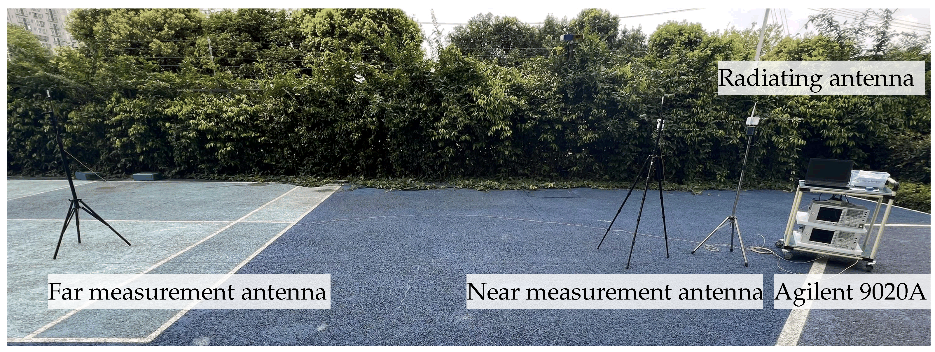
4.1. Experiment Description

In order to verify the effectiveness and performance of the proposed $E^{2}ISA$, which aims to solve the aviation equipment EMC problem, a group of environmental interference suppression experiments was conducted in an open area, operating at a VHF (approximately 100 MHz), as shown in Figure 5.

Two Agilent 9020A signal analyzers [24] were used to acquire the near and far EMC signals by connecting to two omnidirectional antennas with a frequency scope of 20 MHz to 500 MHz whose gains are the same at different directions. The test frequency covered the FM broadcast frequency band to generate external far-site interference signals. Near-site interference signals were generated by a Agilent 8267D PSG Vector Signal Generator [25], which generated near-site interference signals of different frequencies. Before testing, it was necessary to perform the calibration by placing the near-testing and far-testing antennas together to eliminate the offset of the different equipment. Similar to the literature [10], all antennas in our experiments remained stationary during each test.

The one-meter and three-meter methods were both used in the tests. In the one-meter test, the near-site antenna was placed one meter away from the radiating antenna, and the far-site antenna was located nine meters away from the radiating antenna. In the three-meter test, the near-site antenna was placed three meters away from the radiating antenna, and the far-site antenna was placed nine meters away from the radiating antenna.

After data acquisition, we selected 129 waterfall images at random as the training set, which was labeled by the “labelme” tool, as shown in Figure 6. Horizontal and vertical reflections were carried out on the training set for data augmentation.

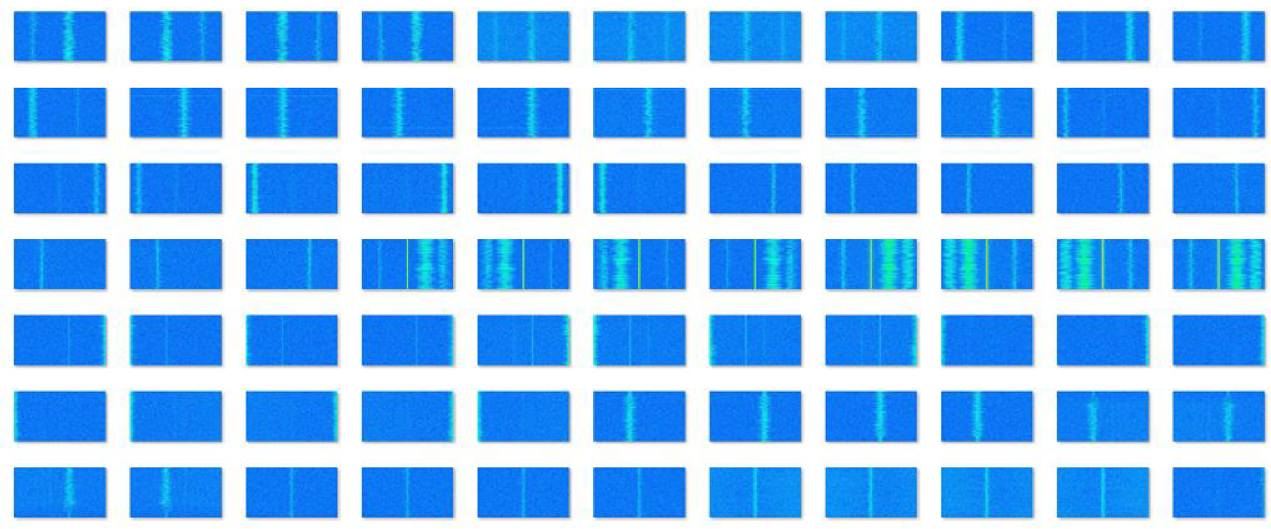
4.2. Analysis of Segmentation Performance

In the open-area EMC testing, the signal might be a single-frequency or a narrow-band signal, which expresses differences in the waterfall images and the effect of the testing parameters, and will be discussed in the following sub-section in detail. As shown in Figure 7, when there is only one single-frequency signal or one narrow-band signal in the waterfall, the segmentation method behaves well, and the segmentation region can completely cover the original signal accurately.

The segmentation results of the multiple-signal waterfall images are shown in Figure 8, which includes a single-frequency signal and three narrow-band signals. The second one is rather dimmer than the others. As can be seen from Figure 8, each signal is segmented successively. Compared to the single-signal case, the multiple signals have less effect on the segmentation performance. Furthermore, there is no adhesion among different signals, which is crucial for the following operation based on the connectivity.

In some special cases, an incomplete signal appears at the edge of the waterfall image, which is shown in Figure 9. From the result, we find that sound segmentation results can still be achieved, which shows the robustness of the proposed method. Furthermore, we find that some tiny pieces appear in the segmentation result corresponding to a very dim signal (almost invisible to the naked eye). Theoretically, they can be suppressed by setting a higher threshold, but this will lead to a loss of sensitivity. Thus, these fragments are retained during segmentation and suppressed during the connectivity detection phase by calculating the area of each segmented region.

4.3. Analysis of Suppression Performance

After segmentation, we compare the corresponding regions of the near-testing and the far-testing images to judge the belongings of each signal. As shown in Figure 10, there are four segments of signals. By comparing the signal bandwidth and energy differences, we find that for the signal in the red box, the energy difference between the near testing and the far testing is huge, which indicates that it is more likely to be a target signal rather than an external interference signal. In contrast, the signal in the black box has a small energy difference between the near and far tests and should therefore be considered external interference and be properly suppressed. This result is shown in Figure 10c.

As shown in Figure 11, there are two time-varying signals generated during experiments. By judging the difference between near and far testing SLTVSF curves using JS divergence, KL divergence, cosine distance, and linear similarity, we state that the left-side signals have different time-varying features and should be judged as internal interference. In contrast, the right-side signals have similar time-varying features and should be judged as external interference.

We use accuracy to assess the effectiveness of segmentation, which refers to the percentage of correctly classified samples in the total samples and is defined as follows:

$$ACC=\frac{n_{\mathrm{correct}}}{n_{\mathrm{total}}},$$

(10)

where $ACC$ denotes the accuracy of segmentation, $n_{\mathrm{correct}}$ denotes the number of correctly classified samples, and $n_{\mathrm{total}}$ denotes the total number of samples.

The internal interference recognition accuracy is counted based on the experiment sets. As shown in

Table 1. Different types of internal interference recognition results.

Signal Class	Single-Frequency	Narrow-Band	Incomplete	Total
Number	4	45	4	53
Correct	4	43	4	51

, we find that the $E^{2}ISA$ accuracy is 96.2%.

Whole-band internal interference testing curves with and without $E^{2}ISA$ are shown in Figure 12. We find that $E^{2}ISA$ can suppress the majority of the external interference and obtain clean EMC testing results.

5. Conclusions

This paper focuses on the open-area environmental interference suppression problem for EMC testing. We find that the proposed $E^{2}ISA$ method, which combines the deep learning segmentation network with the classical recognition methods, can suppress environmental interference signals accurately. Experimental results show that the accuracy of $E^{2}ISA$ reached 96.2% in the face of VHF EMC testing, and all the environmental interference signals were suppressed properly.

References

1. Hinton, G.E.; Osindero, S.; Teh, Y.W. A Fast Learning Algorithm for Deep Belief Nets. Neural Comput. 2006, 18, 1527–1554. [Google Scholar] [CrossRef] [PubMed]
2. Liu, S.W.; Li, M.; Duan, X.T. A Hybrid Model for Semantic Image Segmentation. In Proceedings of the 2015 3rd International Symposium on Computer, Communication, Control and Automation (3CA 2015), Paris, France, 9–10 August 2015; Information Engineering Research Institute: Weimar, TX, USA, 2015; p. 6. [Google Scholar]
3. Sharma, R.; Saqib, M.; Lin, C.T.; Blumenstein, M. A Survey on Object Instance Segmentation. SN Comput. Sci. 2022, 3, 499. [Google Scholar] [CrossRef]
4. Roy, R.; Mazumdar, S.; Chowdhury, A.S. ADGAN: Attribute-Driven Generative Adversarial Network for Synthesis and Multiclass Classification of Pulmonary Nodules. IEEE Trans. Neural Netw. Learn. Syst. 2024, 35, 2484–2495. [Google Scholar] [CrossRef] [PubMed]
5. Arafat, M.Y.; Khairuddin, A.S.M.; Paramesran, R. Connected Component Analysis Integrated Edge Based Technique for Automatic Vehicular License Plate Recognition Framework. IET Intell. Transp. Syst. 2020, 14, 712–723. [Google Scholar] [CrossRef]
6. Daniel, J.; Rose, J.T.A.; Vinnarasi, F.S.F.; Rajinikanth, V. VGG-UNet/VGG-SegNet Supported Automatic Segmentation of Endoplasmic Reticulum Network in Fluorescence Microscopy Images. Scanning 2022, 2022, 7733860. [Google Scholar] [CrossRef] [PubMed]
7. Ganesan, G.; Chinnappan, J. Hybridization of Resnet with Yolo Classifier for Automated Paddy Leaf Disease Recognition: An Optimized Model. J. Field Robot. 2022, 39, 1085–1109. [Google Scholar] [CrossRef]
8. Near and Far Field. 2024. Available online: https://en.wikipedia.org/w/index.php?title=Near_and_far_field&oldid=1195279418 (accessed on 17 January 2024).
9. Wibowo, I.A.; Jenu, M.Z.M.; Alireza, C. Preliminary Design and Development of Open Field Antenna Test Site. Int. J. Integr. Eng. 2010, 2, 3. [Google Scholar]
10. Handlon, D. Radiated Emissions Measurements in an Open Area Test Site. 2010. Available online: https://www.cenam.mx/sm2010/info/pjueves/sm2010-jp06d.pdf (accessed on 17 January 2024).
11. Yadavendra; Chand, S. Semantic Segmentation of Human Cell Nucleus Using Deep U-Net and Other Versions of U-Net Models. Netw. Comput. Neural Syst. 2022, 33, 167–186. [Google Scholar] [CrossRef]
12. Han, L.; Li, X.; Dong, Y. Convolutional Edge Constraint-Based U-Net for Salient Object Detection. IEEE Access 2019, 7, 48890–48900. [Google Scholar] [CrossRef]
13. Liu, Y. Multisource Information Data Fusion Based on Adaptive Least Mean Square Error Algorithm. Comput. Informatiz. Mech. Syst. 2022, 5, 42–44. [Google Scholar]
14. Pan, L.; Chen, K.; Zheng, Z.; Zhao, Y.; Yang, P.; Li, Z.; Wu, S. Aging of Chinese Bony Orbit: Automatic Calculation Based on Unet++ and Connected Component Analysis. Surg. Radiol. Anat. 2022, 44, 749–758. [Google Scholar] [CrossRef] [PubMed]
15. Boraik, O.; Manjunath, R.; Saif, M. Characters Segmentation from Arabic Handwritten Document Images: Hybrid Approach. Int. J. Adv. Comput. Sci. Appl. 2022, 13, 2022. [Google Scholar] [CrossRef]
16. Diao, Z.; Sun, F. Visual Object Tracking Based on Deep Neural Network. Math. Probl. Eng. 2022, 2022, 2154463. [Google Scholar] [CrossRef]
17. Dass, J.M.A.; Kumar, S.M. A Novel Approach for Small Object Detection in Medical Images Through Deep Ensemble Convolution Neural Network. Int. J. Adv. Comput. Sci. Appl. 2022, 13. [Google Scholar] [CrossRef]
18. Doube, M. Multithreaded Two-Pass Connected Components Labelling and Particle Analysis in Imagej. R. Soc. Open Sci. 2021, 8, 201784. [Google Scholar] [CrossRef] [PubMed]
19. Pediredla, A.; Veeraraghavan, A.; Gkioulekas, I. Ellipsoidal Path Connections for Time-Gated Rendering. ACM Trans. Graph. 2019, 38, 1–12. [Google Scholar] [CrossRef]
20. Sudario, G.; Toohey, S.; Wiechmann, W.; Smart, J.; Boysen-osborn, M.; Youm, J.; Spann, S.; Wray, A. The Applied Weighted Slide Metric (AWSM) Tool: Creation of a Standard Slide Design Rubric. J. Adv. Med Educ. Prof. 2022, 10, 91–98. [Google Scholar] [CrossRef] [PubMed]
21. Chen, J.; Li, P.; Fang, W.; Zhou, N.; Yin, Y.; Zheng, H.; Xu, H.; Wang, R. Fuzzy Frequent Pattern Mining Algorithm Based on Weighted Sliding Window and Type-2 Fuzzy Sets over Medical Data Stream. Wirel. Commun. Mob. Comput. 2021, 2021, e6662254. [Google Scholar] [CrossRef]
22. Sahu, S.P.; Londhe, N.D.; Verma, S.; Agrawal, P.; Banchhor, S.K. False Positives Reduction in Pulmonary Nodule Detection Using a Connected Component Analysis-Based Approach. Int. J. Biomed. Eng. Technol. 2022, 39, 131–148. [Google Scholar] [CrossRef]
23. Kumar, A.; Yin, B.; Shaikh, A.M.; Ali, M.; Wei, W. Corrnet: Pearson Correlation Based Pruning for Efficient Convolutional Neural Networks. Int. J. Mach. Learn. Cybern. 2022, 13, 3773–3783. [Google Scholar] [CrossRef]
24. Keysight. N9020A MXA Signal Analyzer, 10 Hz to 26.5 GHz. Available online: https://www.keysight.com/us/en/product/N9020A/mxa-signal-analyzer-10hz-26-5ghz.html (accessed on 17 January 2024).
25. Keysight. E8267D PSG Vector Signal Generator, 100 kHz to 44 GHz. Available online: https://www.keysight.com/us/en/product/E8267D/psg-vector-signal-generator-100-khz-44-ghz.html (accessed on 17 January 2024).
Figure 1. Near–far EMC testing configuration.
Applsci 14 02703 g001
Figure 2. Diagram of E 2 I S A .
Applsci 14 02703 g002
Figure 3. Hybrid segmentation network model.
Applsci 14 02703 g003
Figure 4. Fusion decision logic model.
Applsci 14 02703 g004
Figure 5. Open-area experiment illustration.
Applsci 14 02703 g005
Figure 6. Training set.
Applsci 14 02703 g006
Figure 7. Segmentation results for single signals.
Applsci 14 02703 g007
Figure 8. Segmentation results for multiple signals.
Applsci 14 02703 g008
Figure 9. Segmentation results for abnormal testing.
Applsci 14 02703 g009
Figure 10. Comparison of near–far SA waterfalls and supression results: (a) near-site SA waterfall; (b) far-site SA waterfall; (c) suppression results.
Applsci 14 02703 g010
Figure 11. Signals with time-varying features.
Applsci 14 02703 g011
Figure 12. Whole–band internal interference testing curves with and without E 2 I S A (there are five internal interference signals and massive environmental interference, which are all suppressed clearly): (a) whole–band internal interference testing curves without suppression; (b) whole–band internal interference testing curves with suppression.
Applsci 14 02703 g012