

A Dynamic Analysis Method of Liquid-Filled Containers Considering the Fluid–Structure Interaction


Abstract
1. Introduction
2. The FEA Theory Based on Acoustic Fluid Elements
- (i)
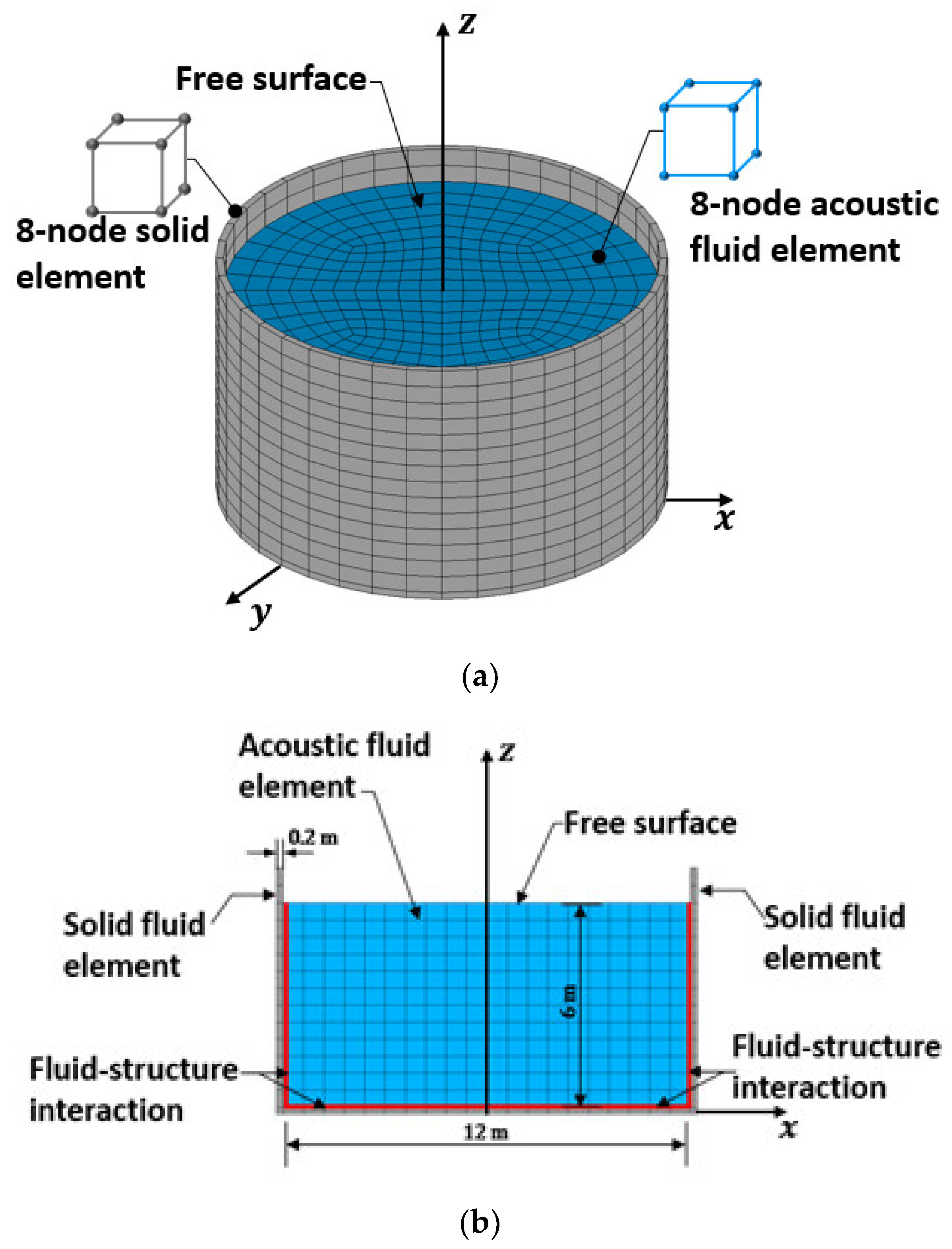
- Fluid–structure interaction: Set a fluid–structure interaction on the boundary between fluid and structure.
- (ii)
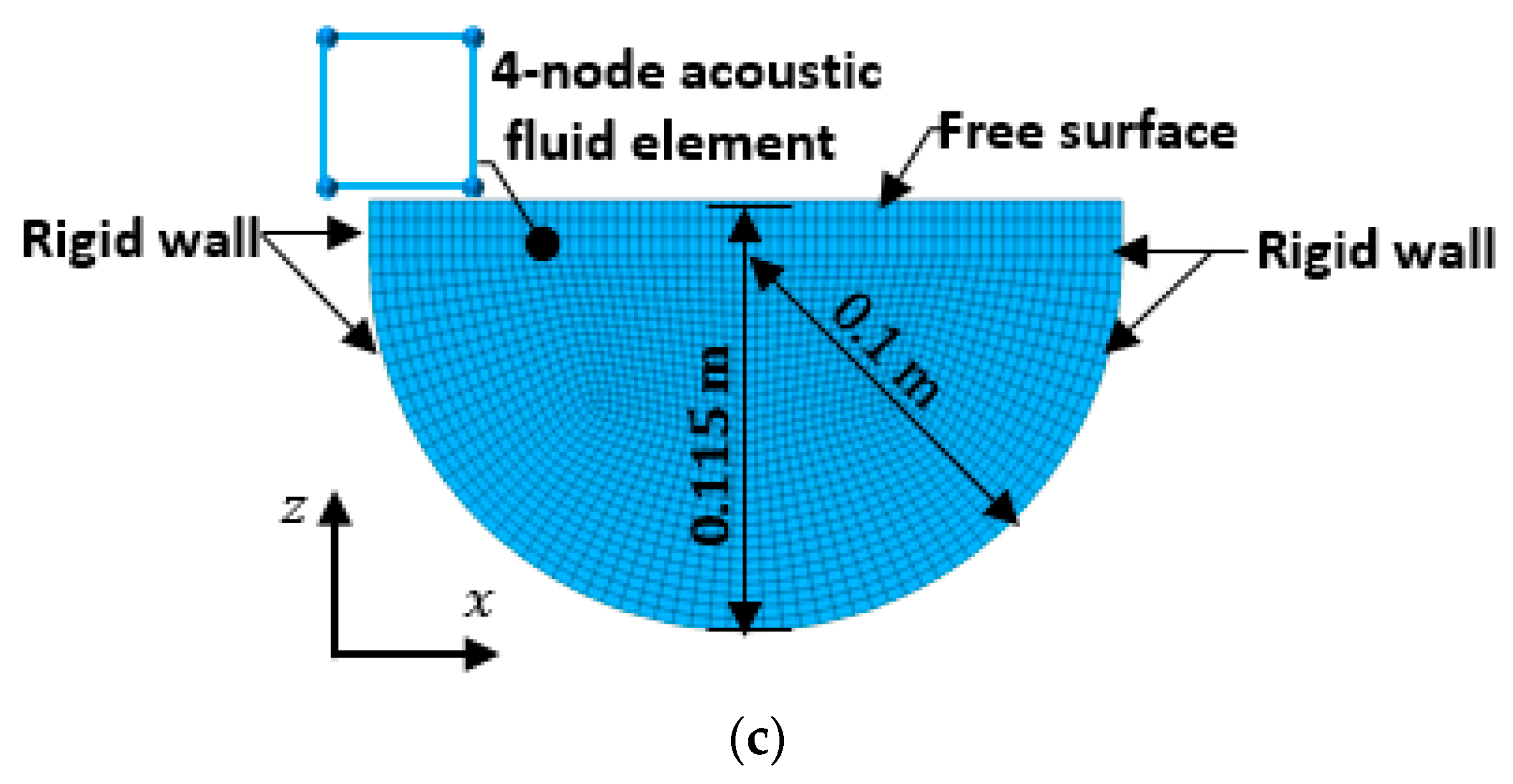
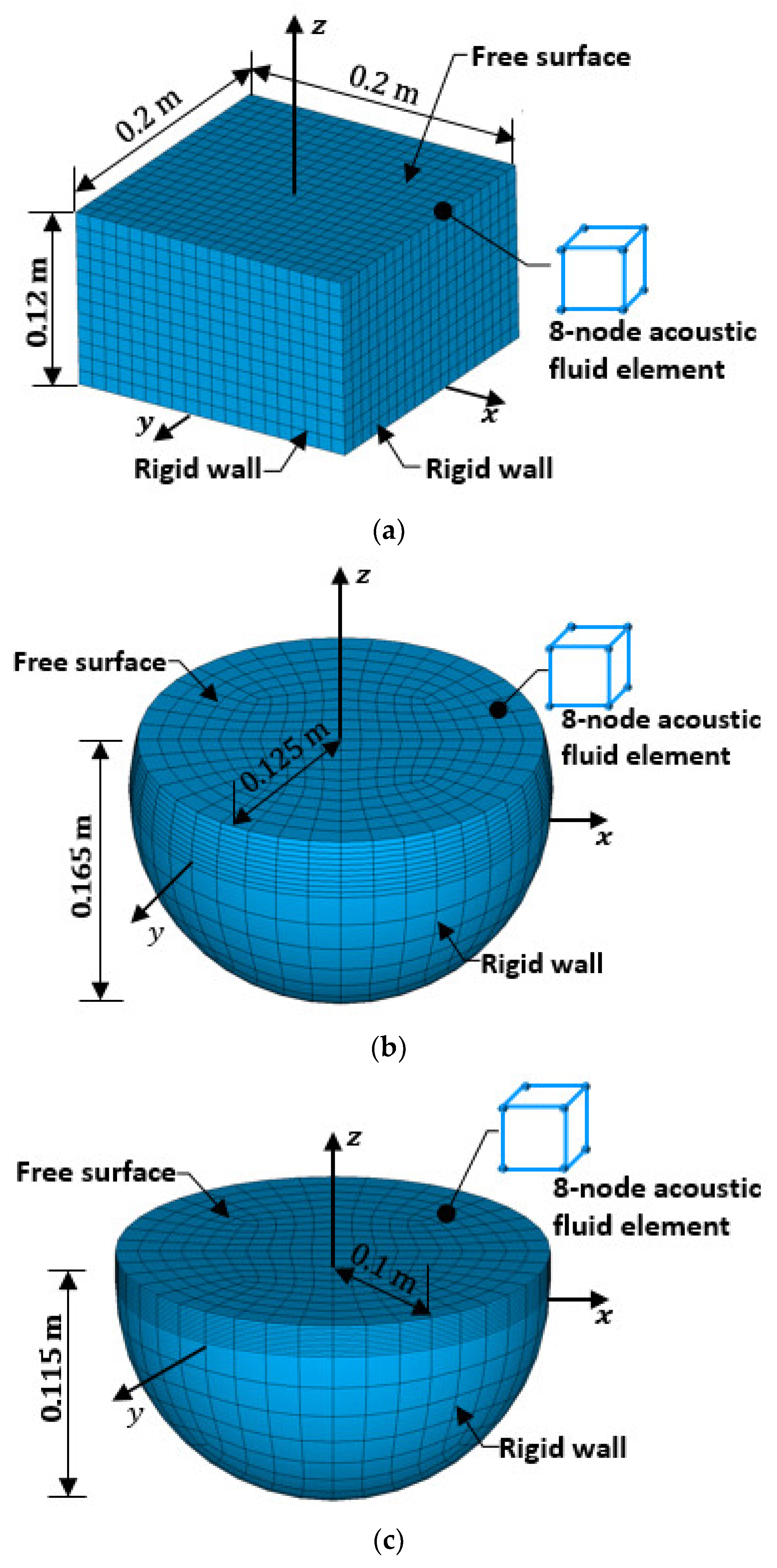
- Free surface: Set a free surface on the top surface of water domain, which can provide an approximate representation of the water surface wave.
- (iii)
- Rigid wall: Set a rigid wall on the bottom and the lateral surface where the water cannot flow through the boundary.
3. Analysis of Liquid Sloshing Modes
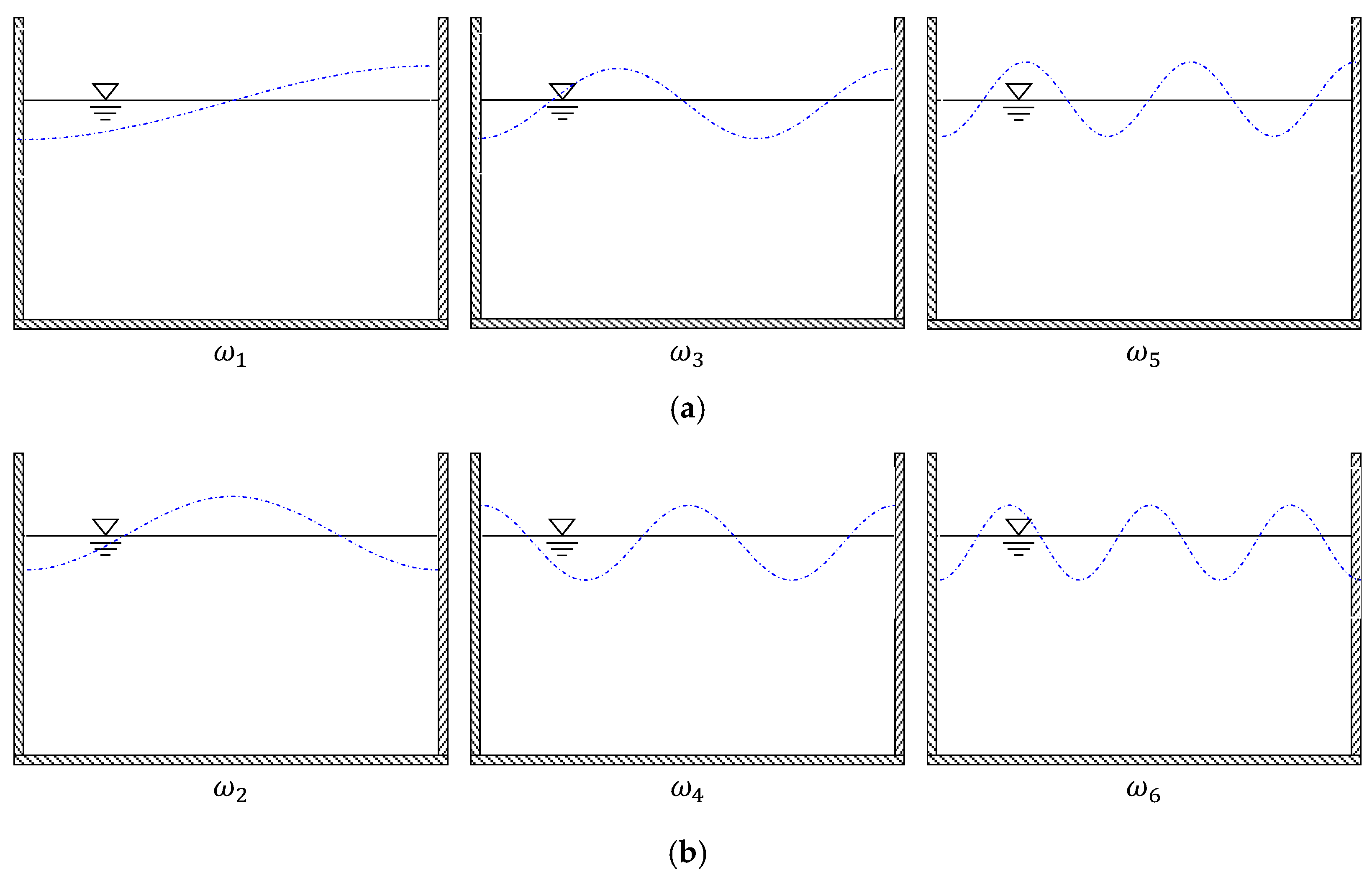
3.1. Theoretical Solutions to 2D Liquid Sloshing Modes
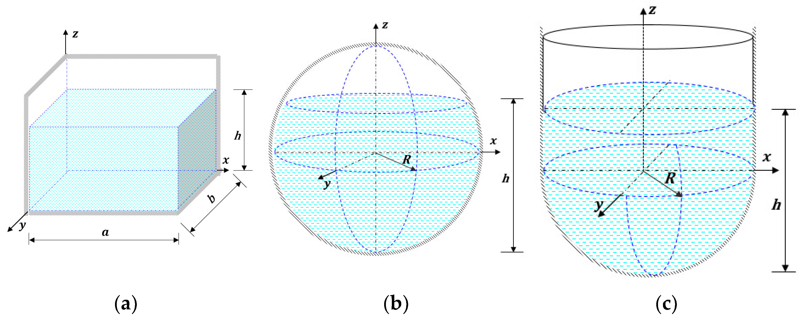
3.1.1. Two-Dimensional Rectangular Container
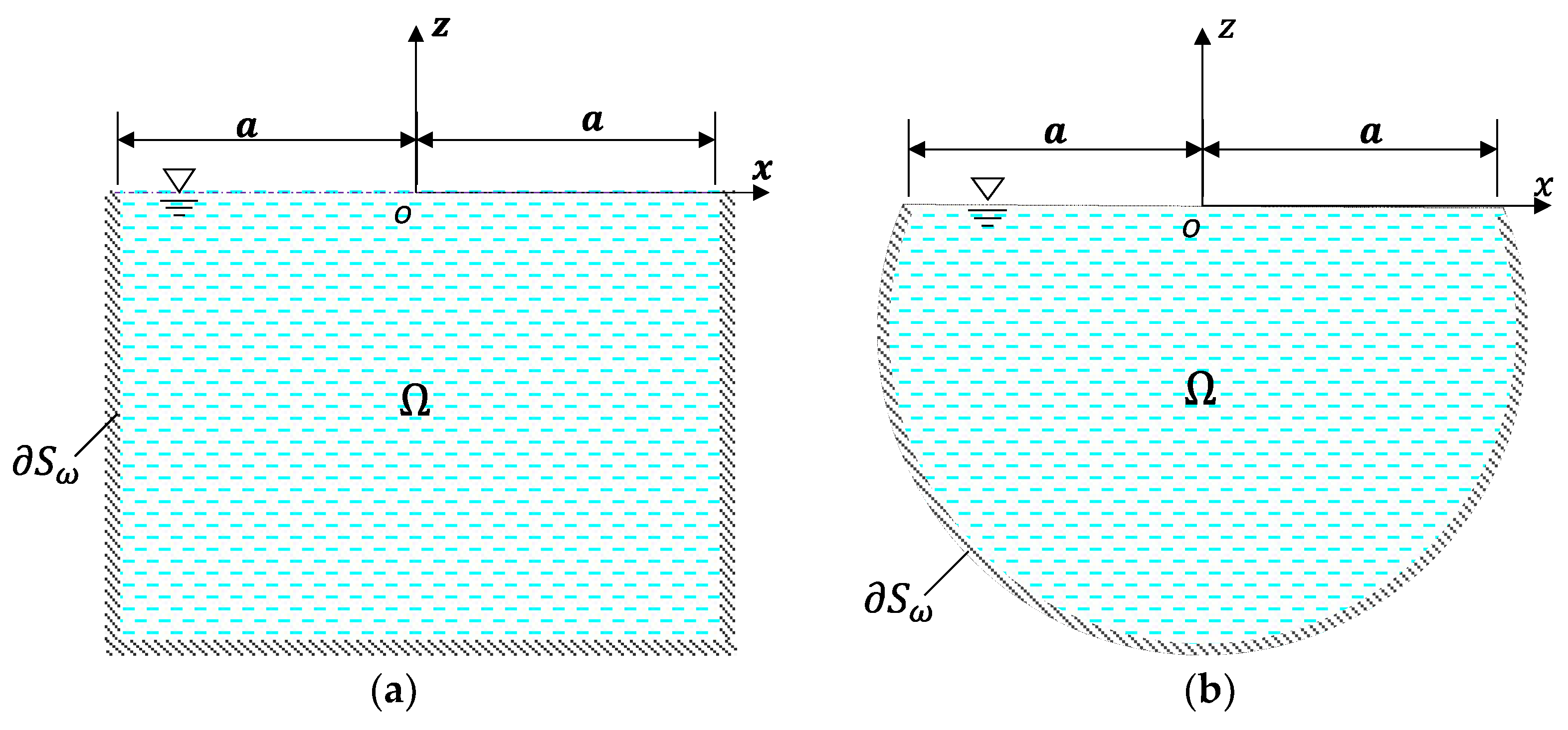
3.1.2. Container with Arbitrary Cross Sections
3.2. FEA of 2D Liquid Sloshing Modes
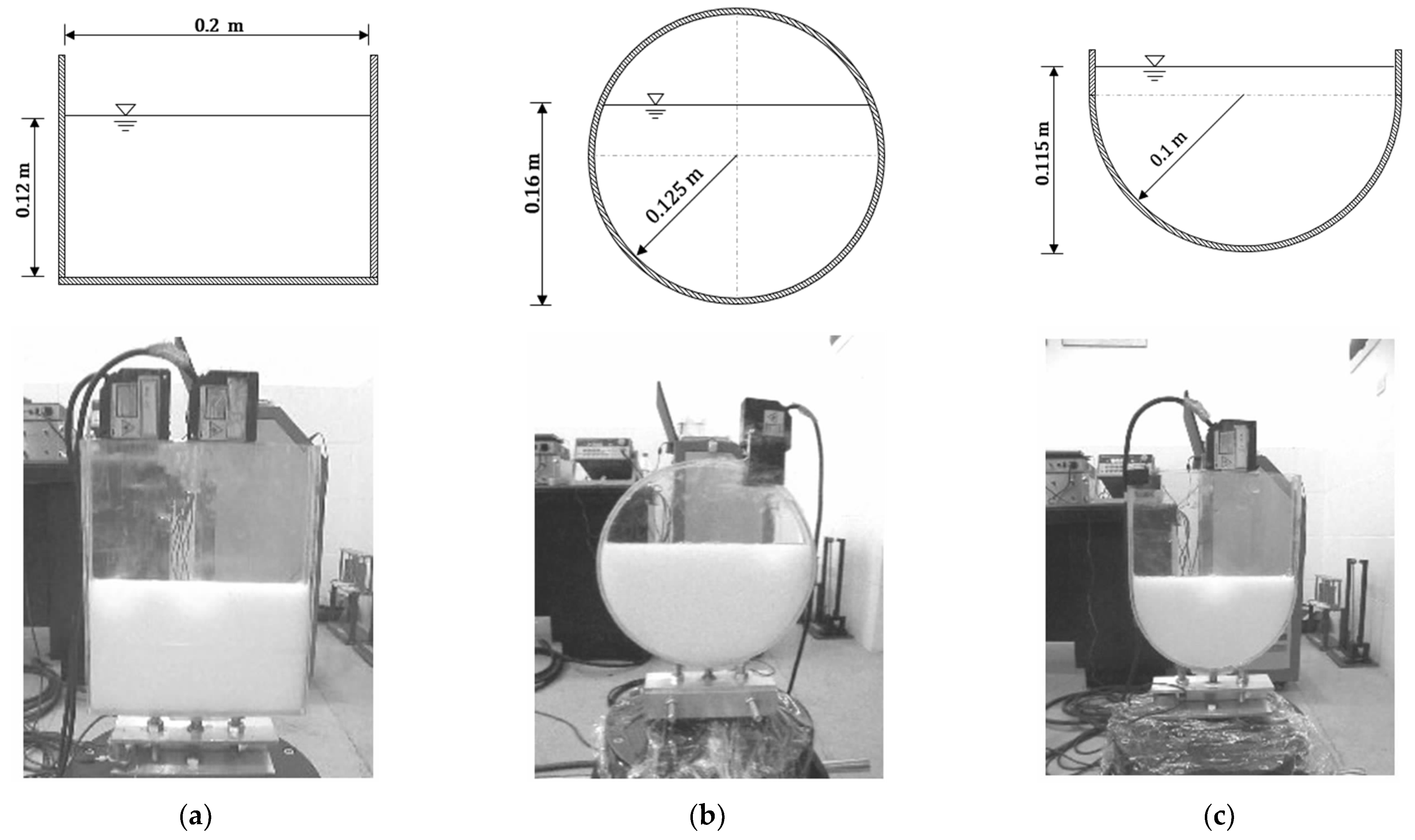
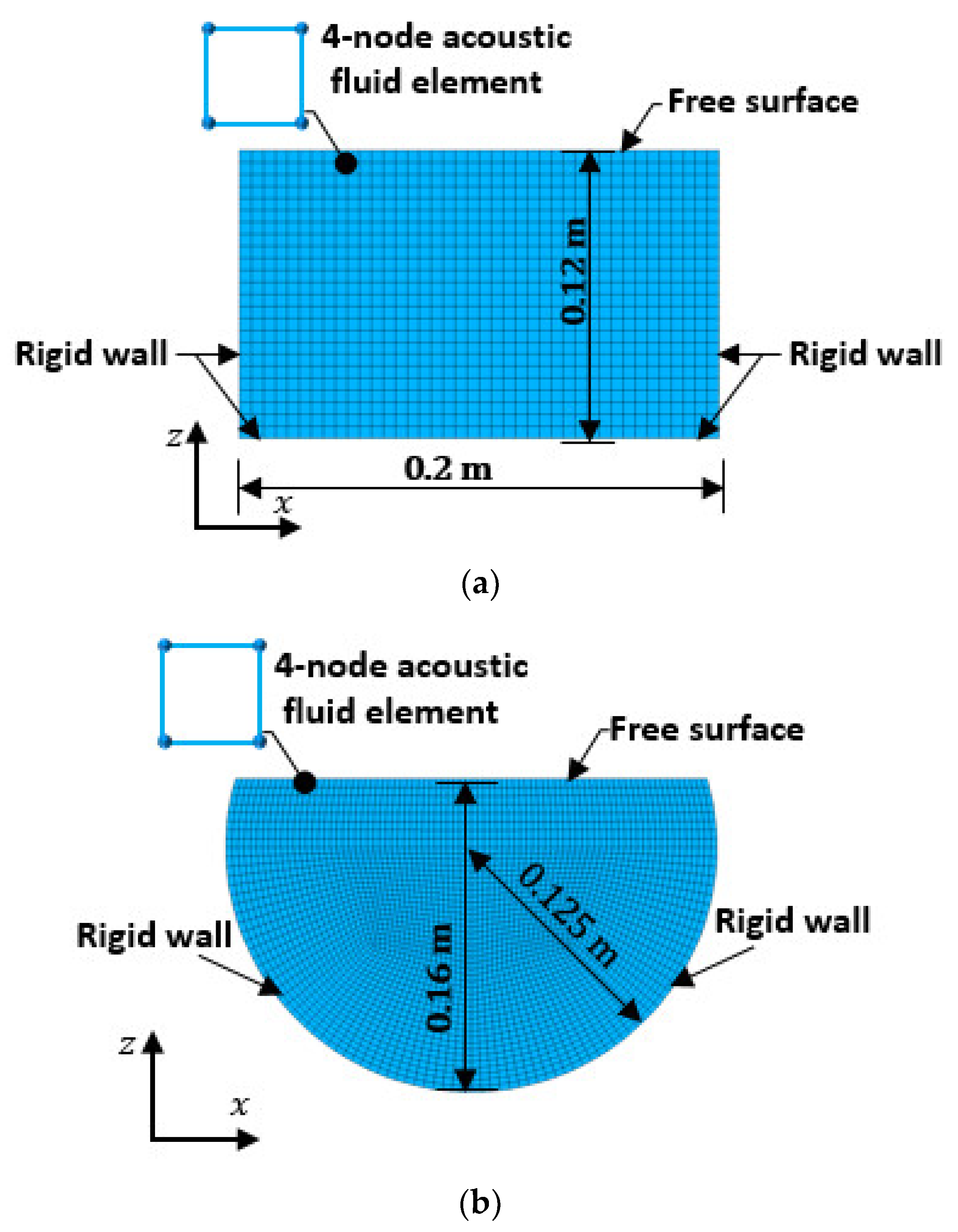
3.2.1. Rectangular Container
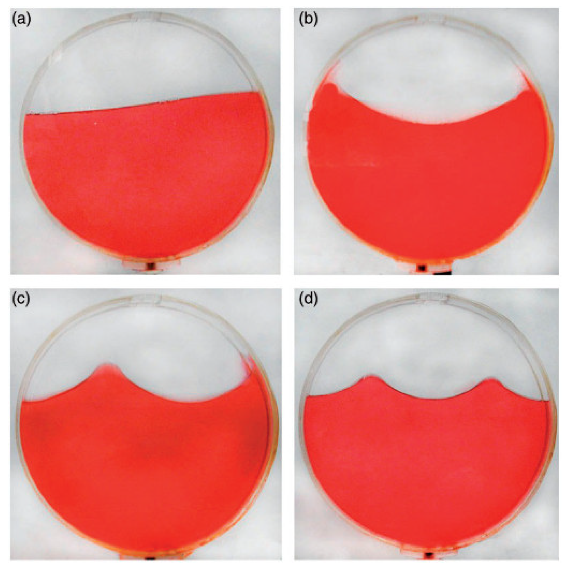
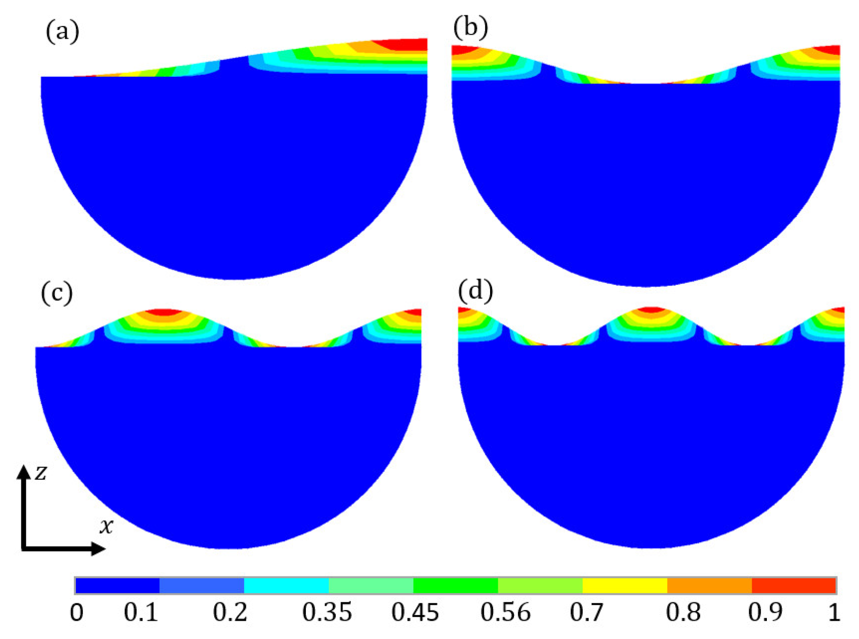
3.2.2. Circular Container
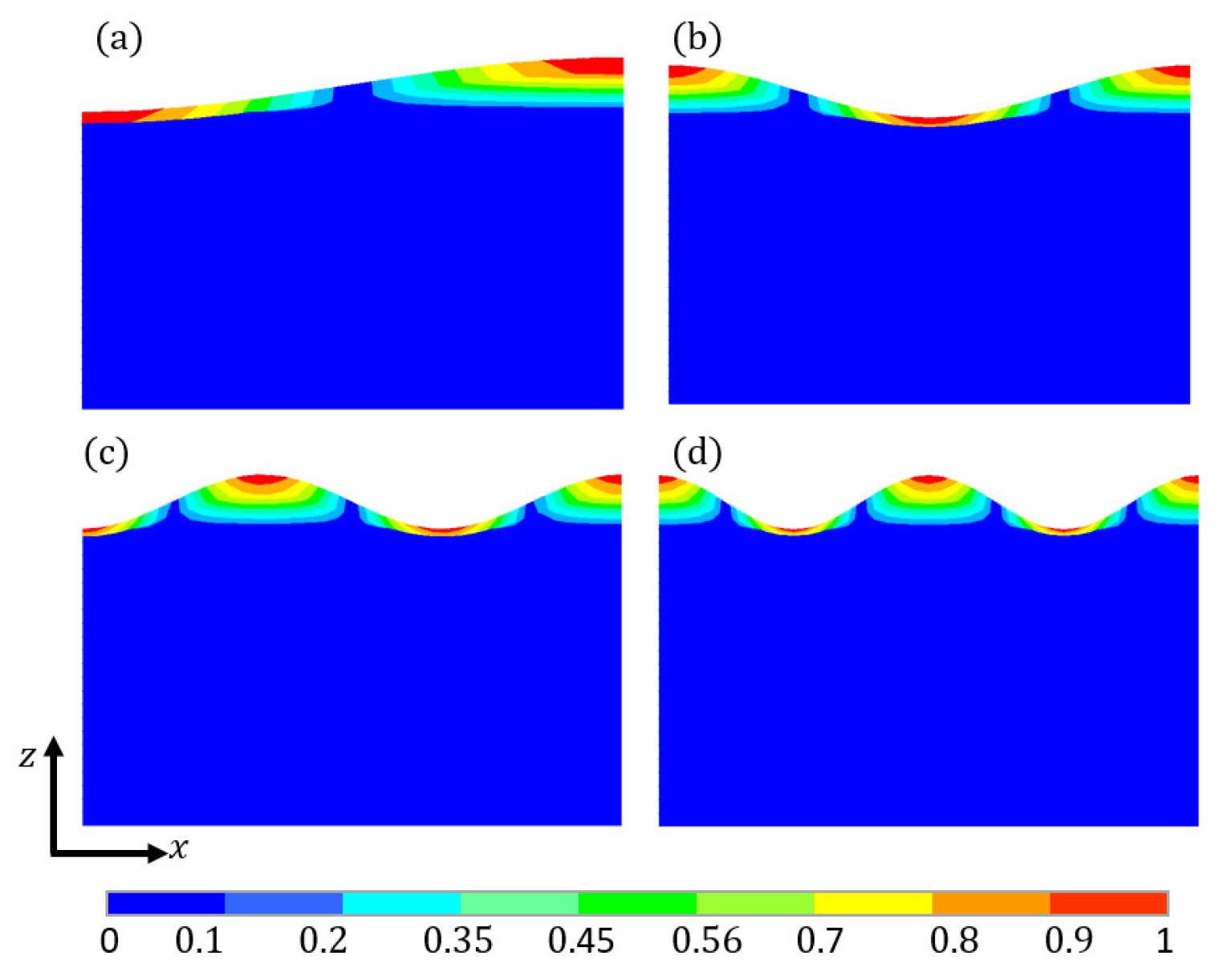
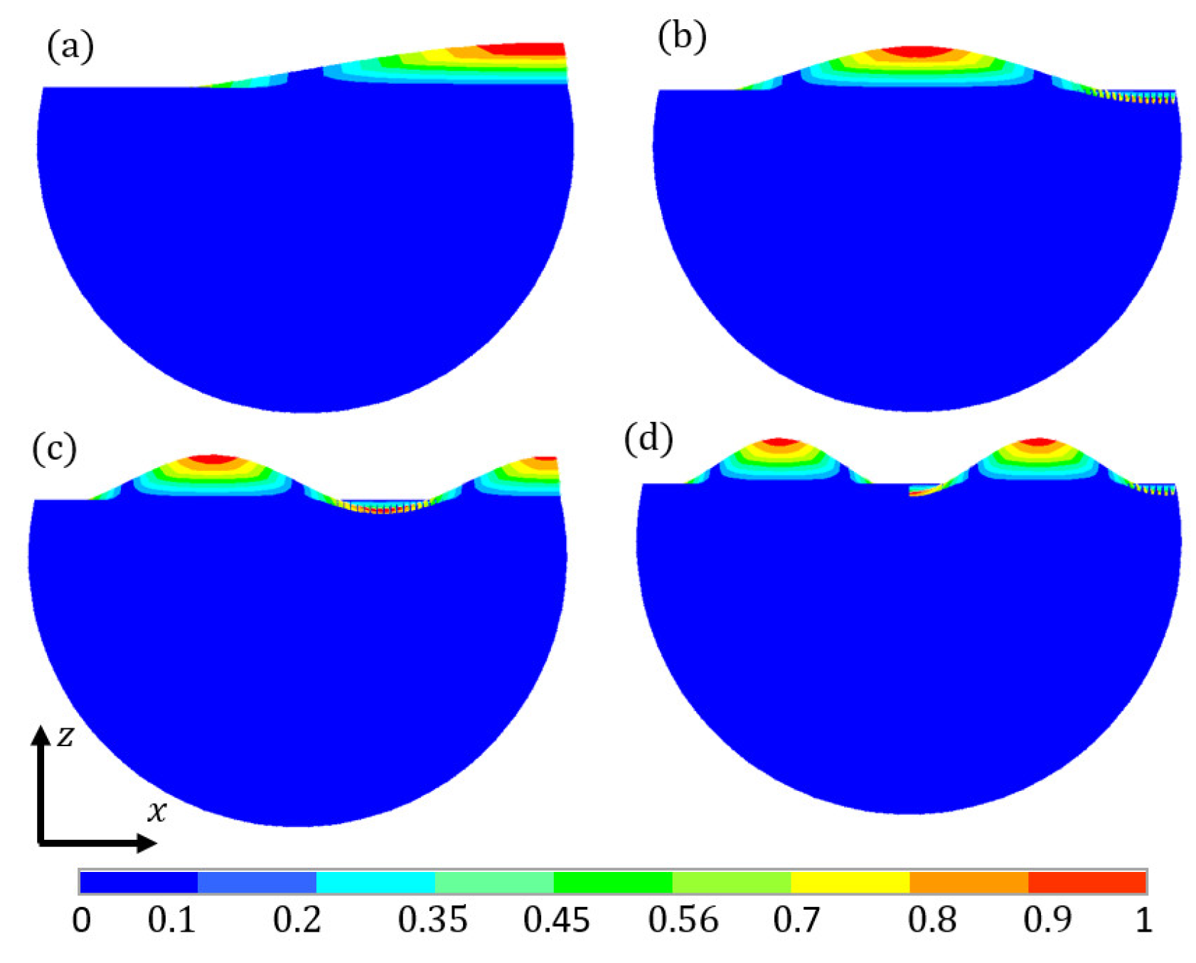
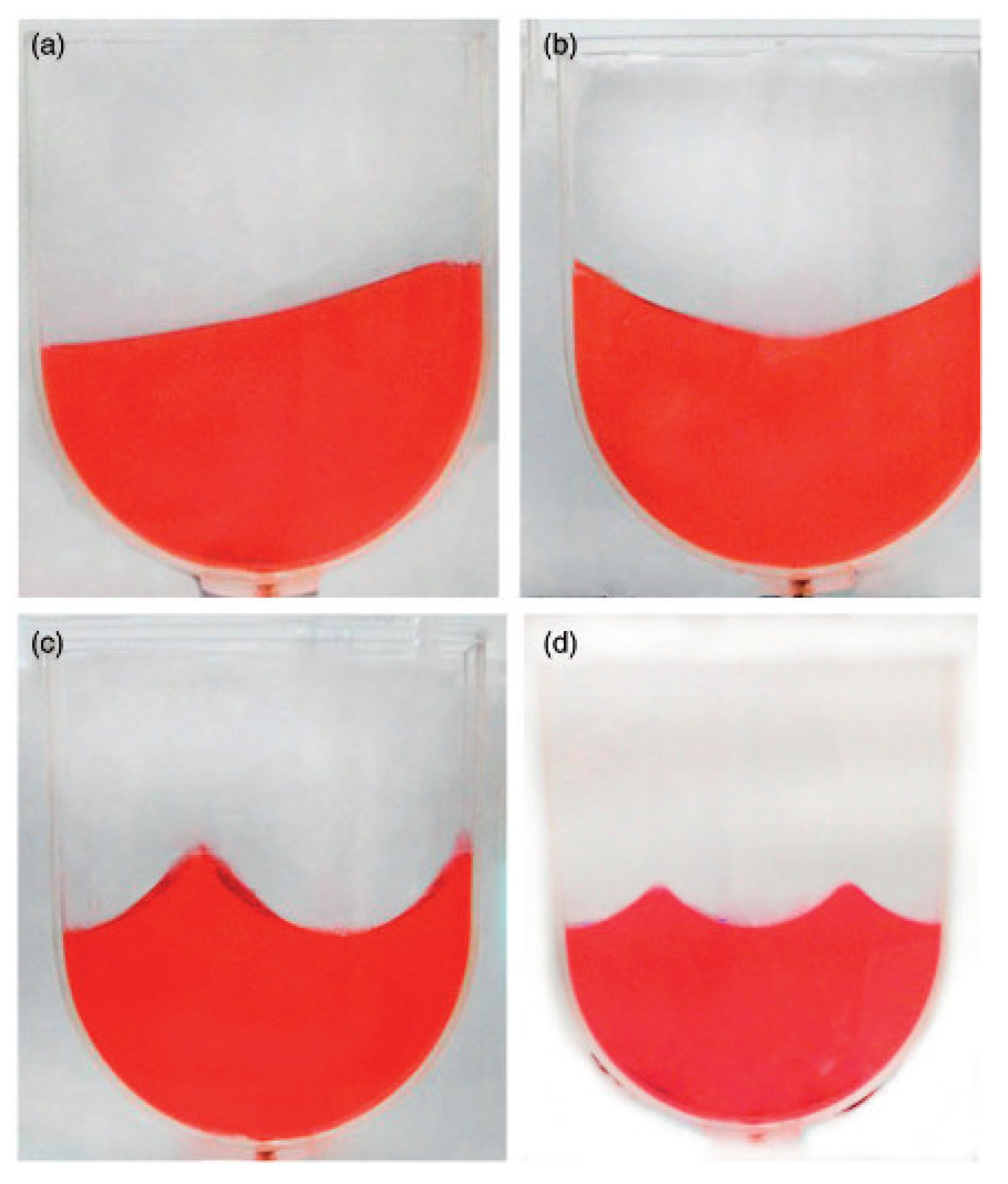
3.2.3. U-Shaped 2D Container
3.3. FEA of 3D Liquid Sloshing Modes
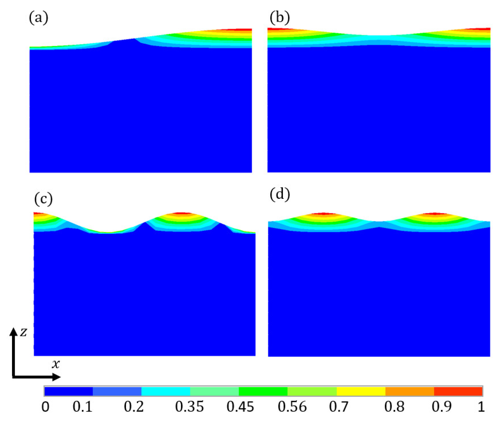
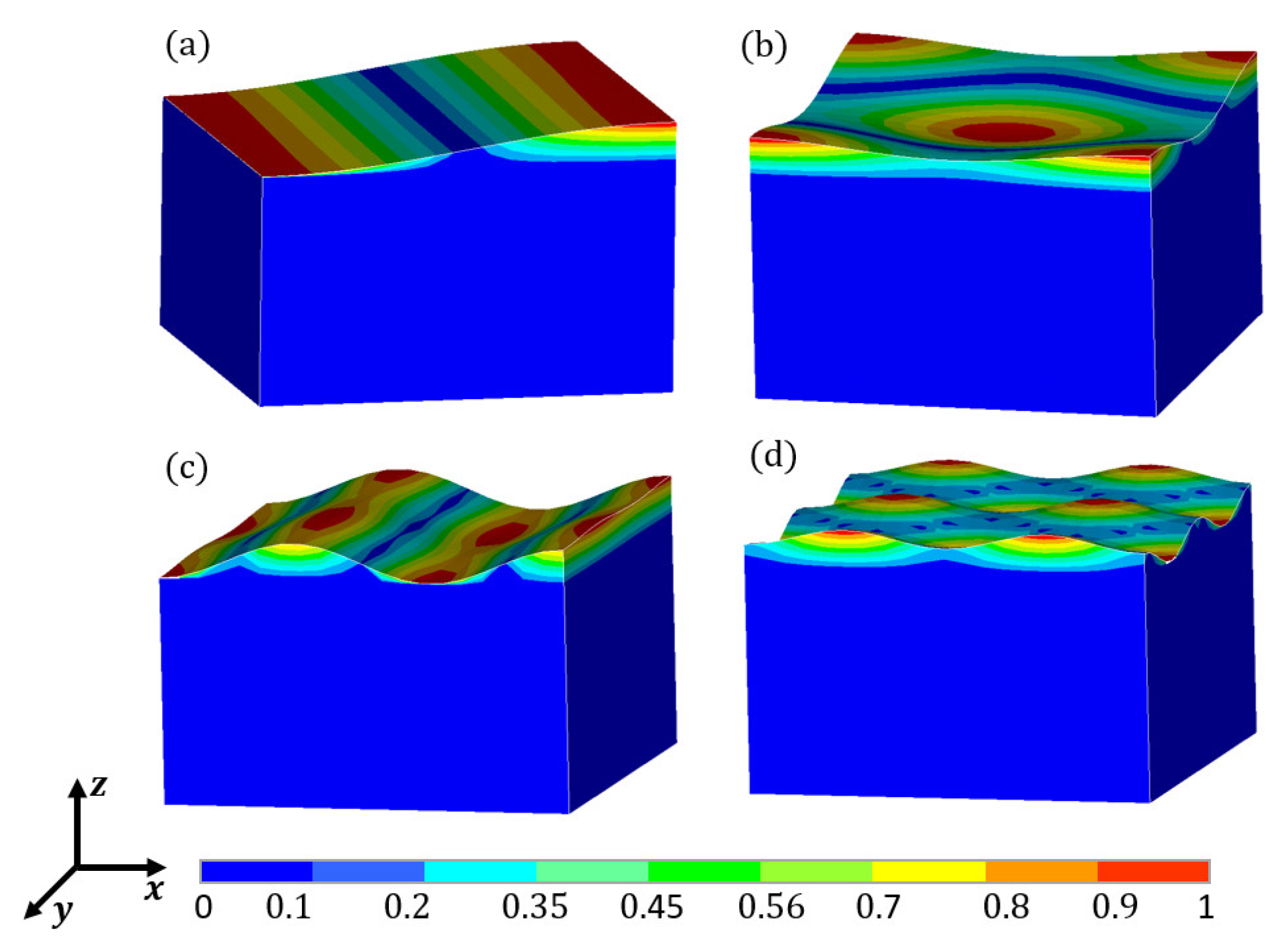
3.3.1. Cuboid Container
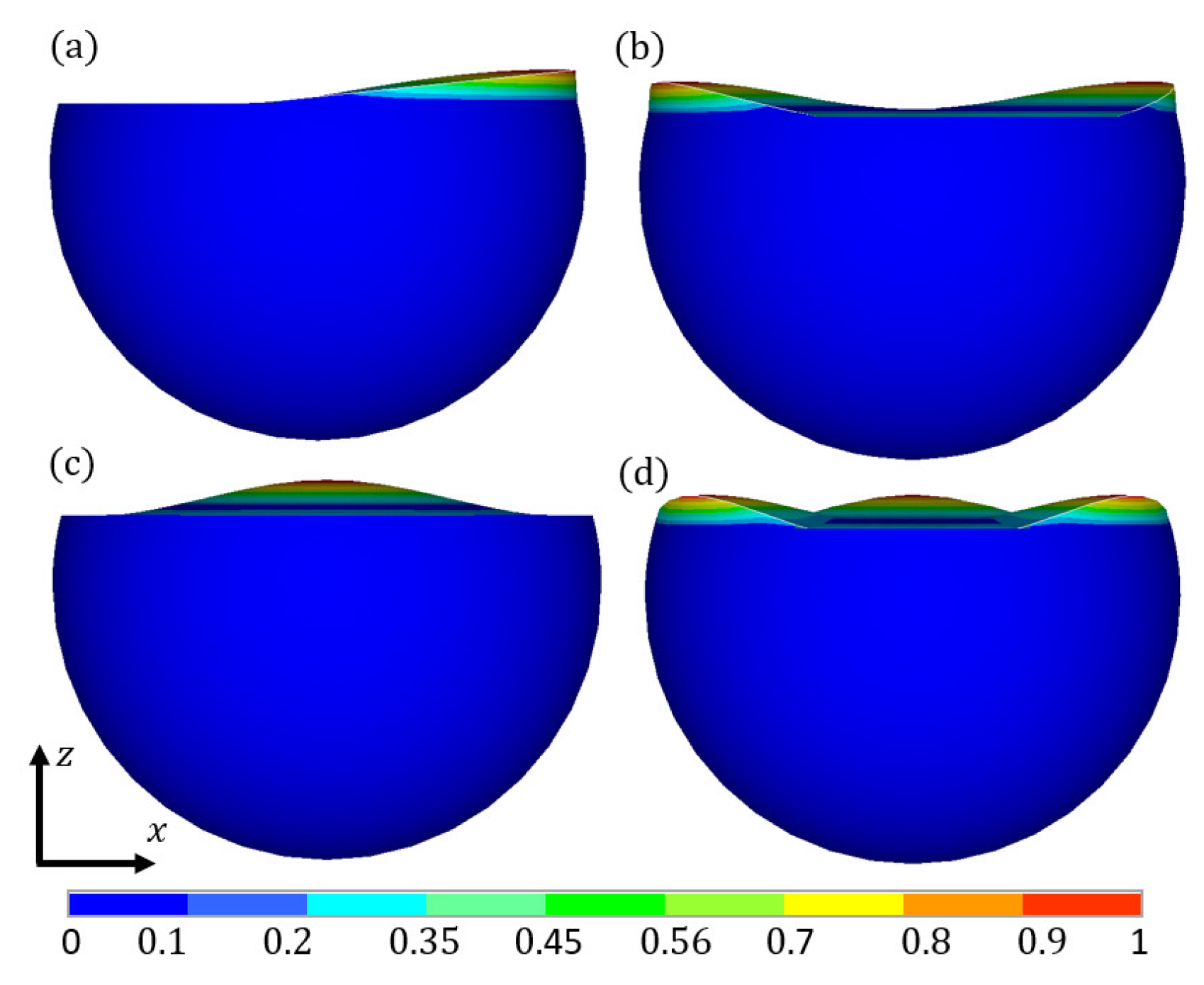
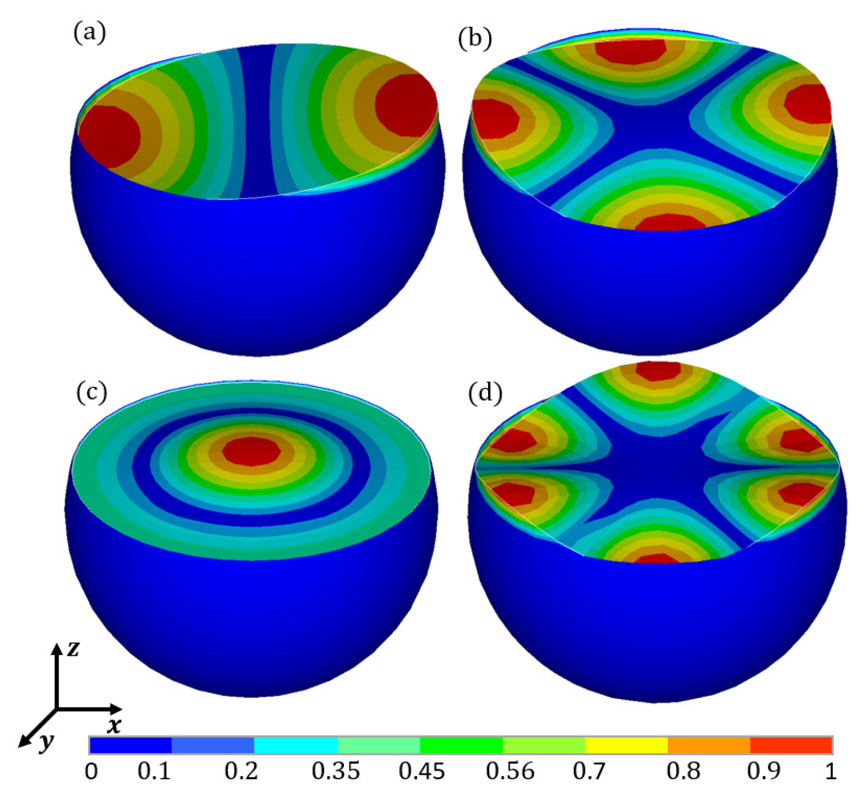
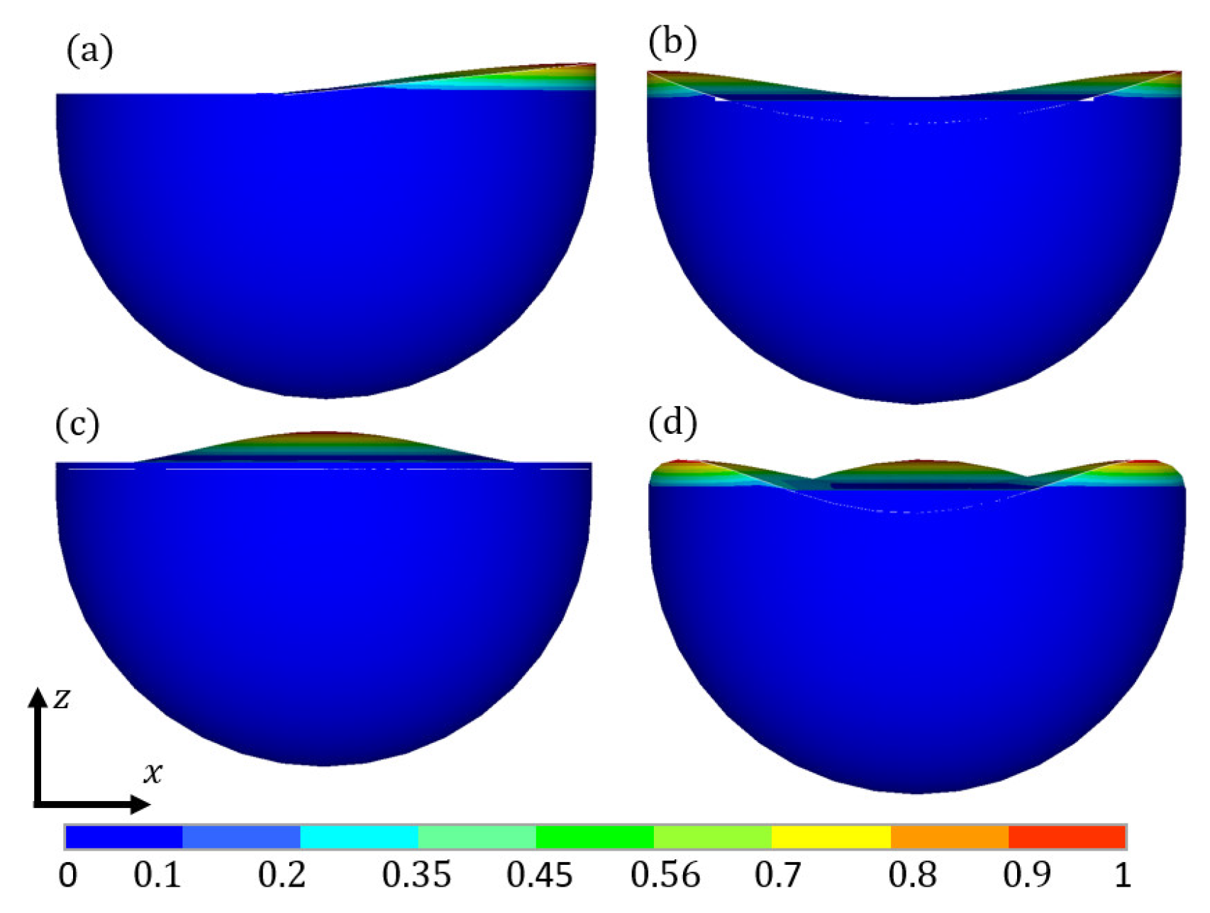
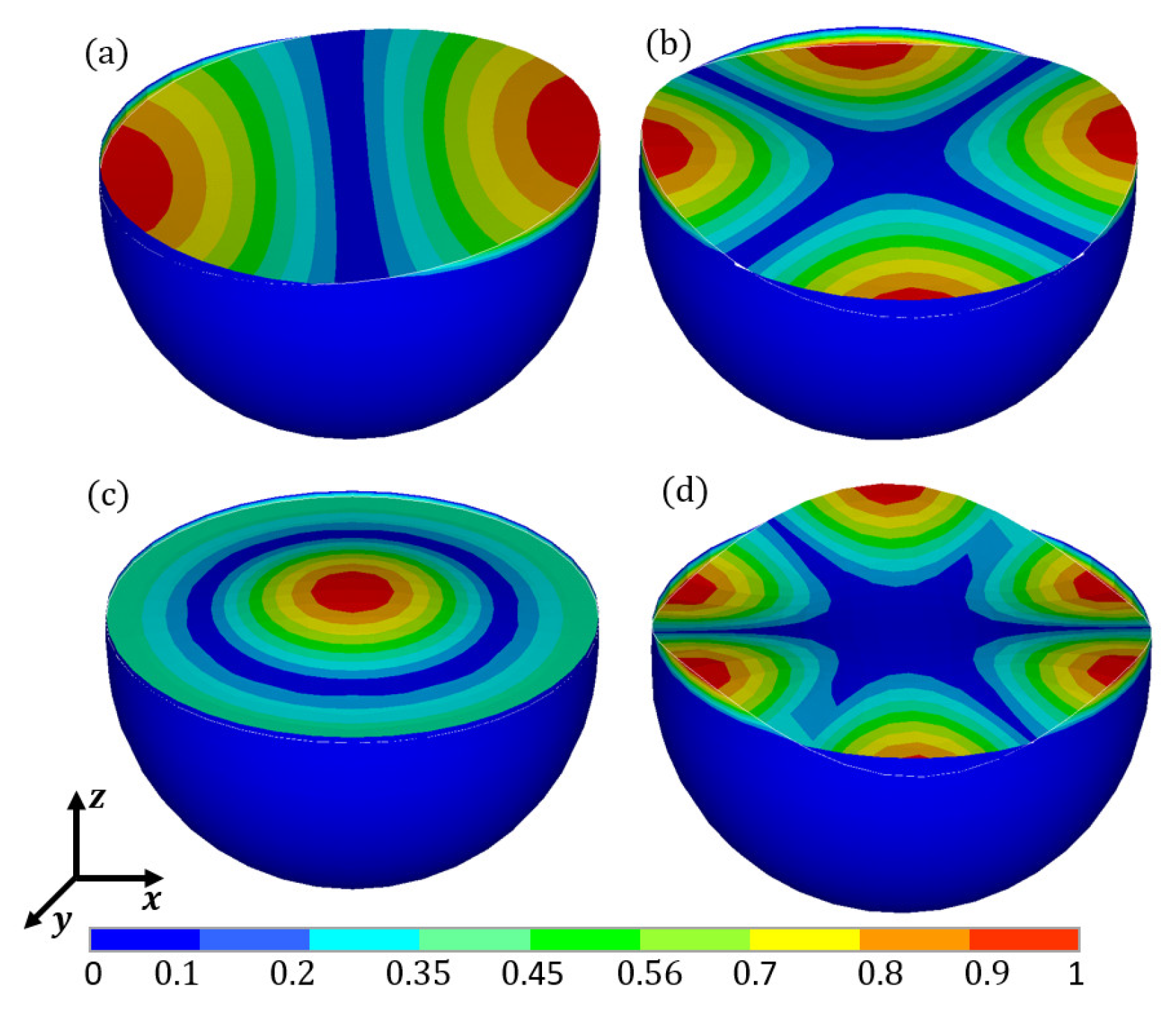
3.3.2. Spherical Container
3.3.3. U-Shaped 3D Container
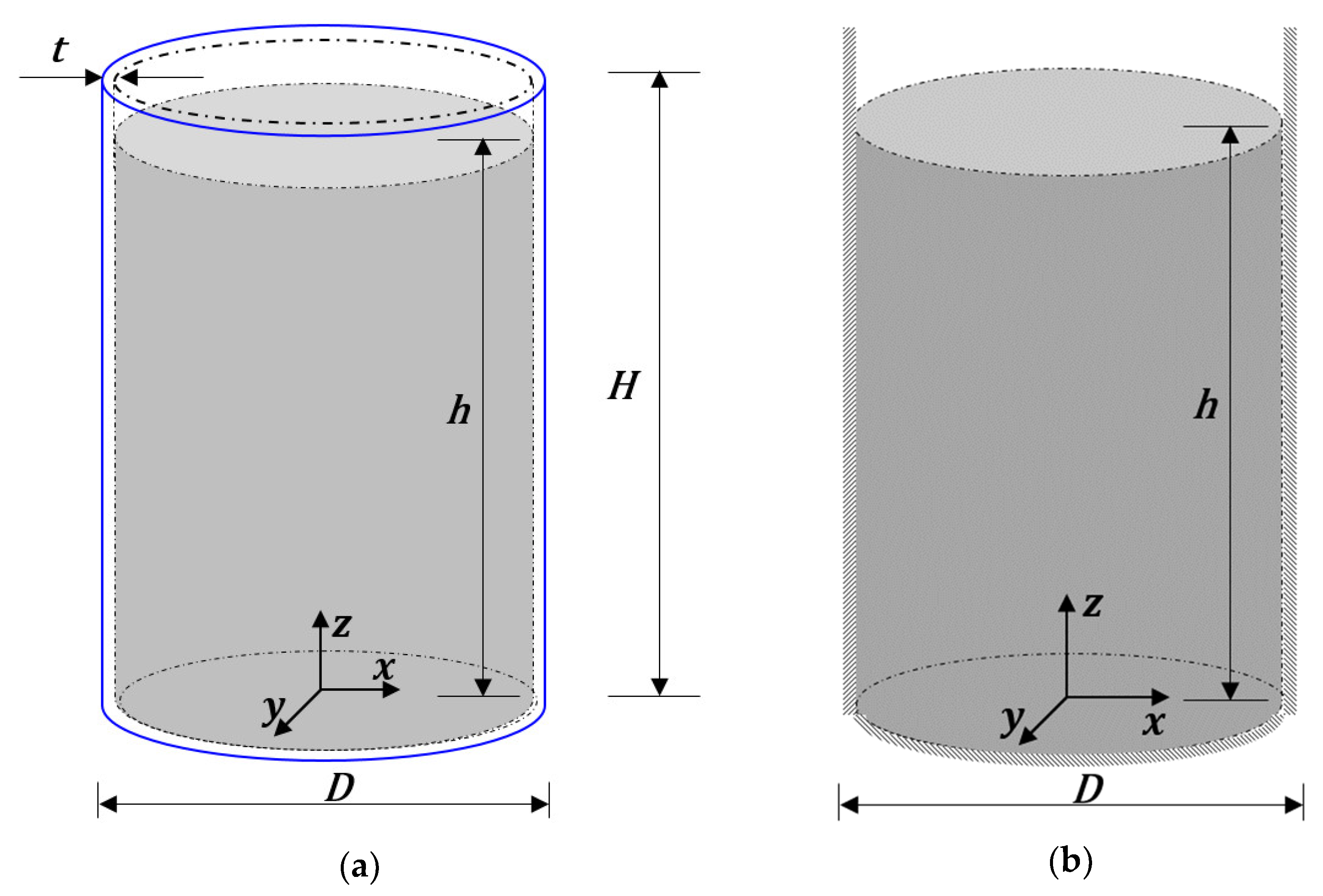
4. Modal Analysis and Time-Historical Analysis of Cylindrical Liquid-Filled Containers
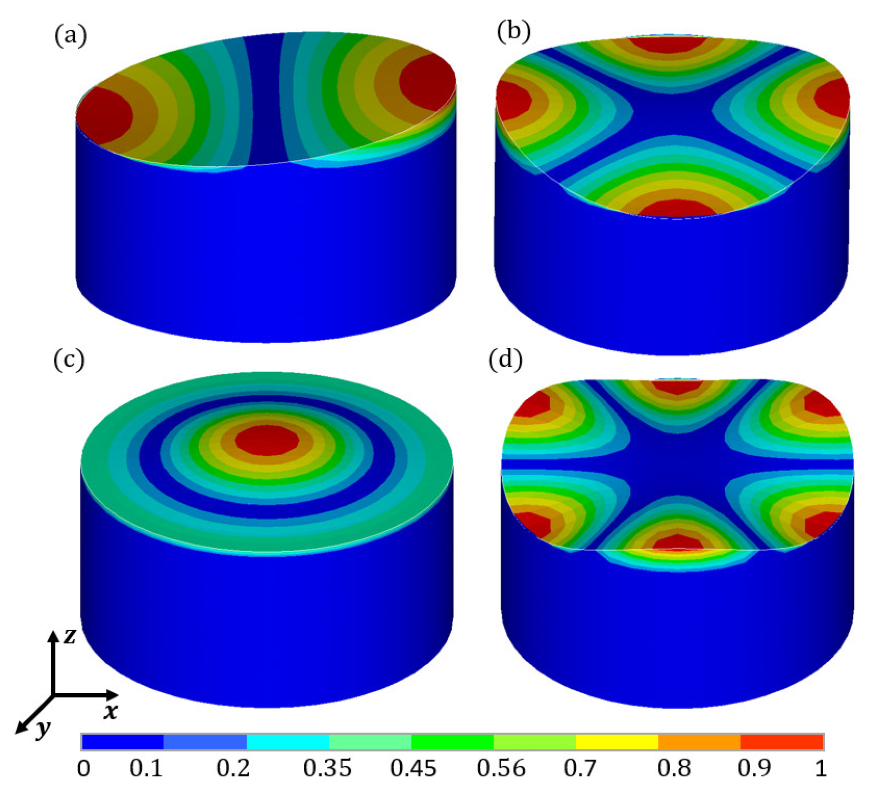
4.1. Liquid Modal Analysis
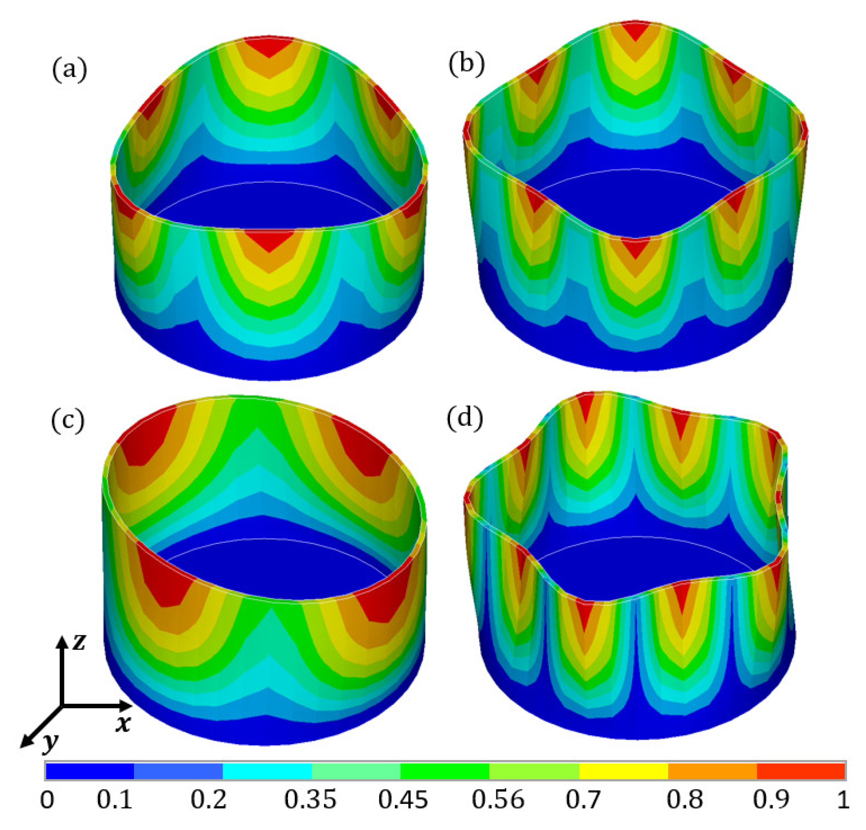
4.2. Modal Analysis of Cylinder Containers
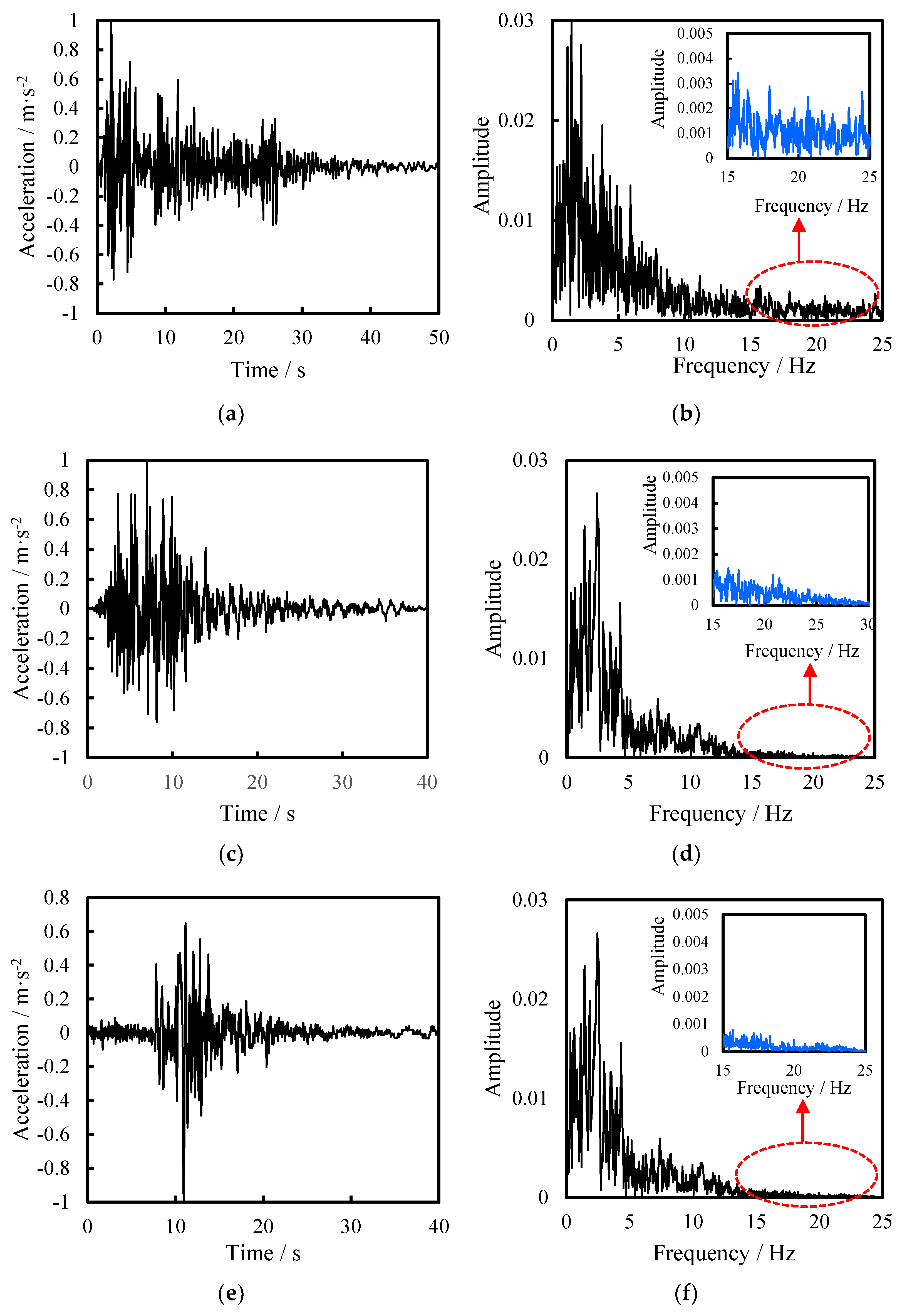
4.3. Time-Historical Analysis of Cylindrical Liquid-Filled Containers
5. Conclusions
- (1)
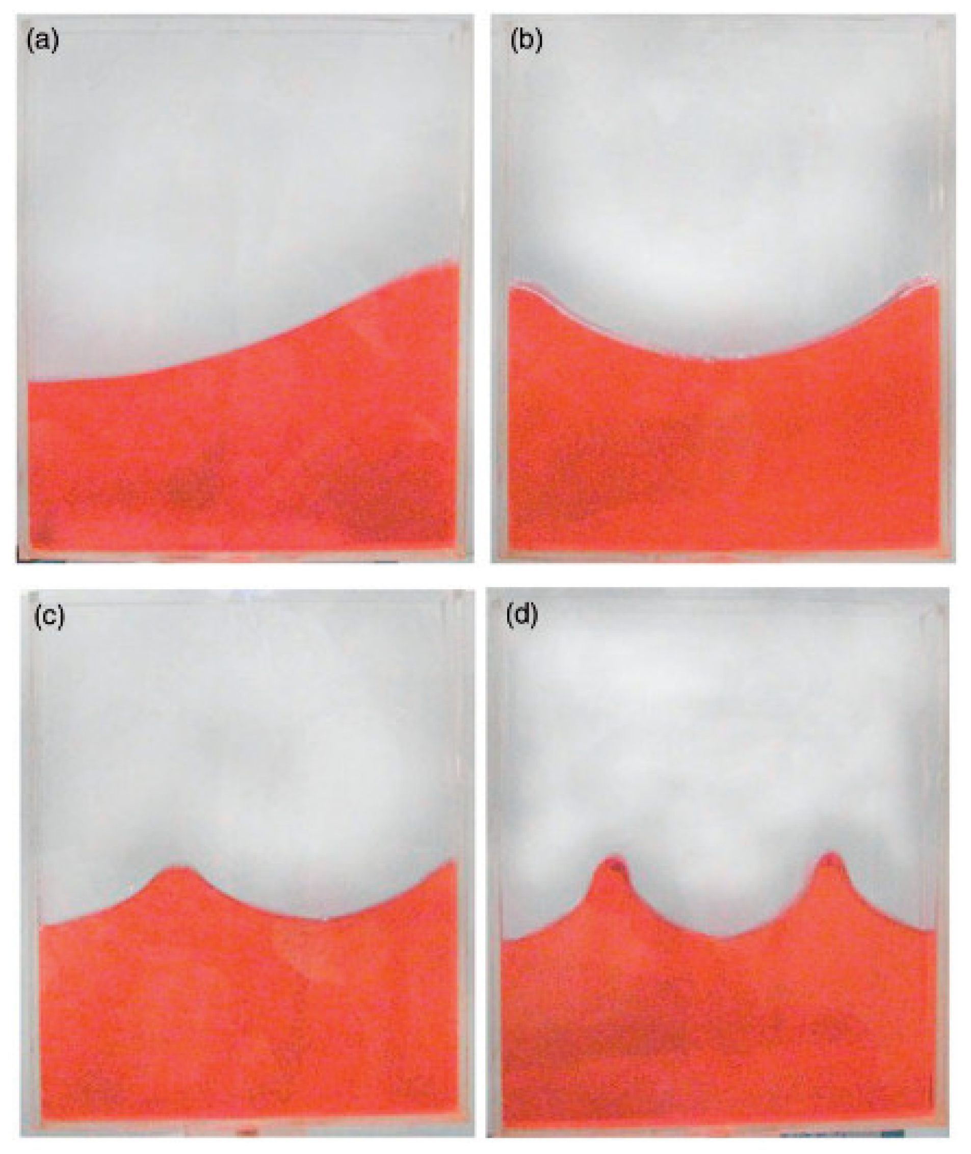
- The liquid sloshing modes in 2D and 3D liquid-filled containers of regular shapes and arbitrary cross sections were analyzed and compared with theoretical solutions and test results. The results reveal that the FEM based on acoustic fluid elements is accurate;
- (2)
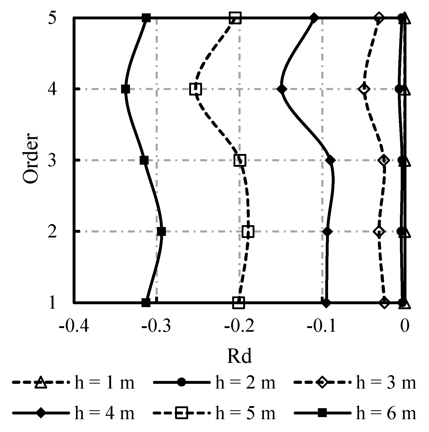
- The liquid level exerts significant influences on the intrinsic frequency of liquid-filled containers. As the liquid level in liquid-filled containers rises, the vibration frequency of cylindrical containers decreases. When the liquid level in liquid-filled containers is 6 m, the first frequency decreases by 31.24%. During the engineering design of such liquid-filled containers, the influence of the effect of FSIs on the intrinsic frequency of these containers should not be ignored. FEM based on acoustic fluid elements can be used to model such an effect;
- (3)
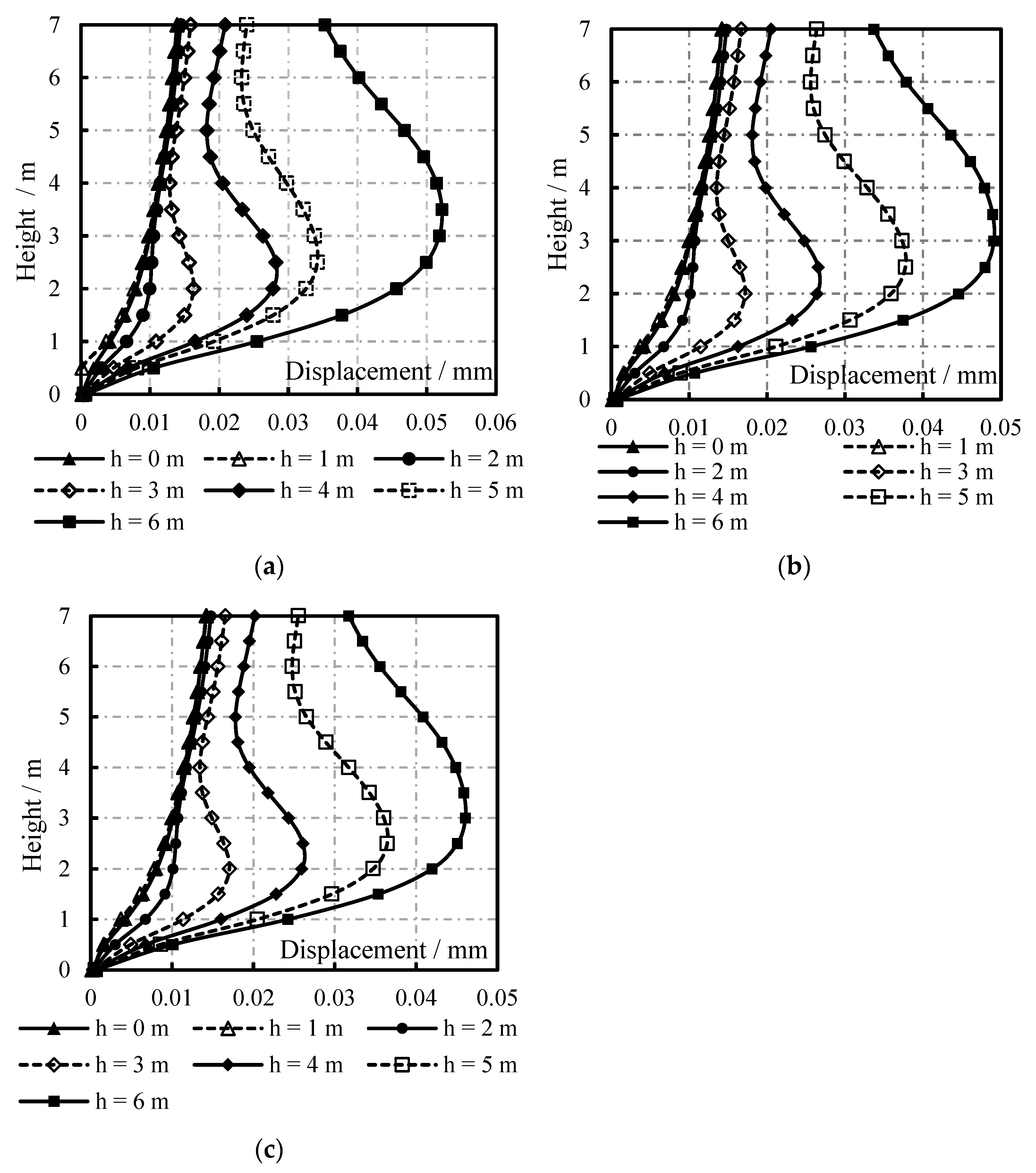
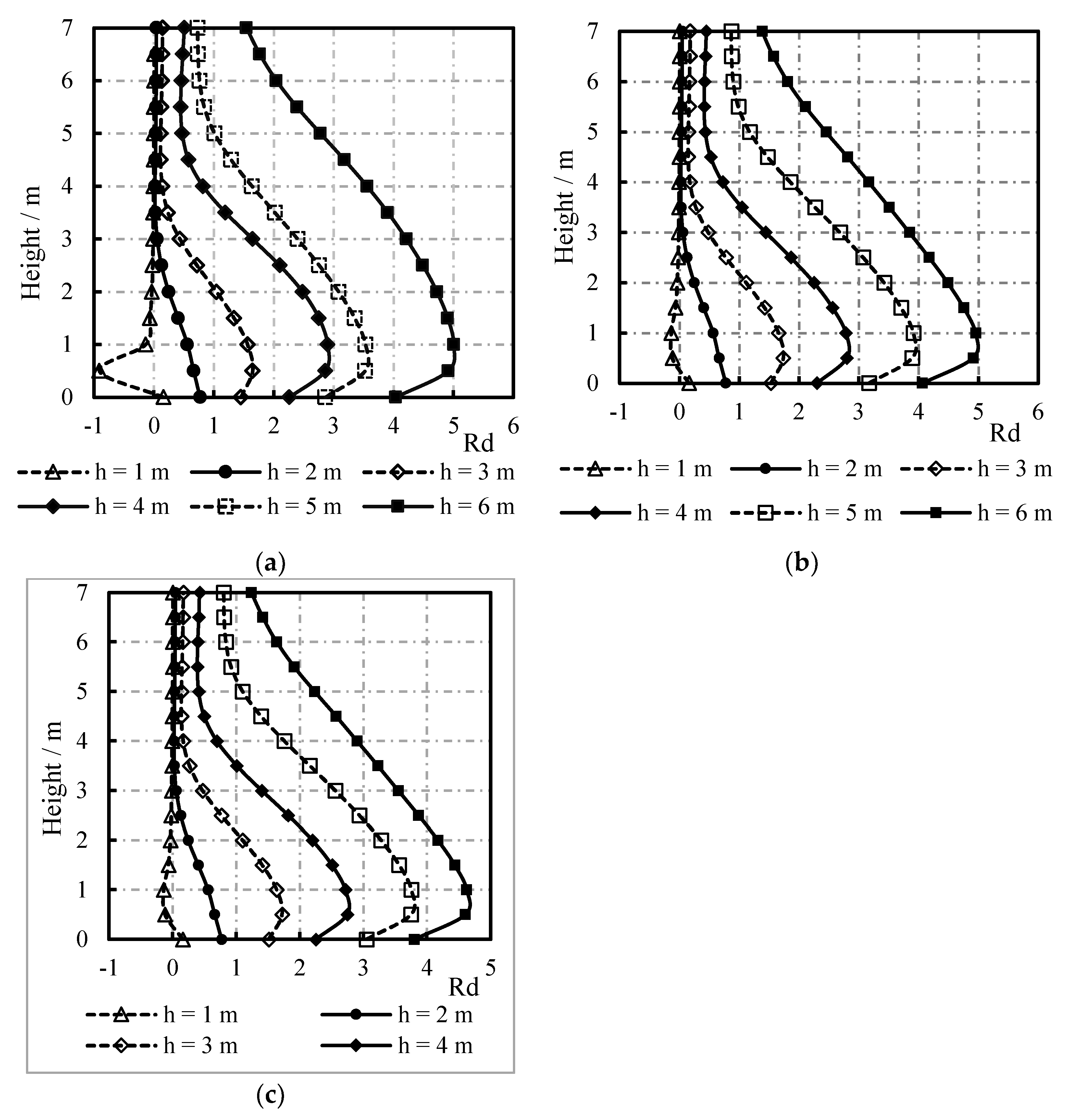
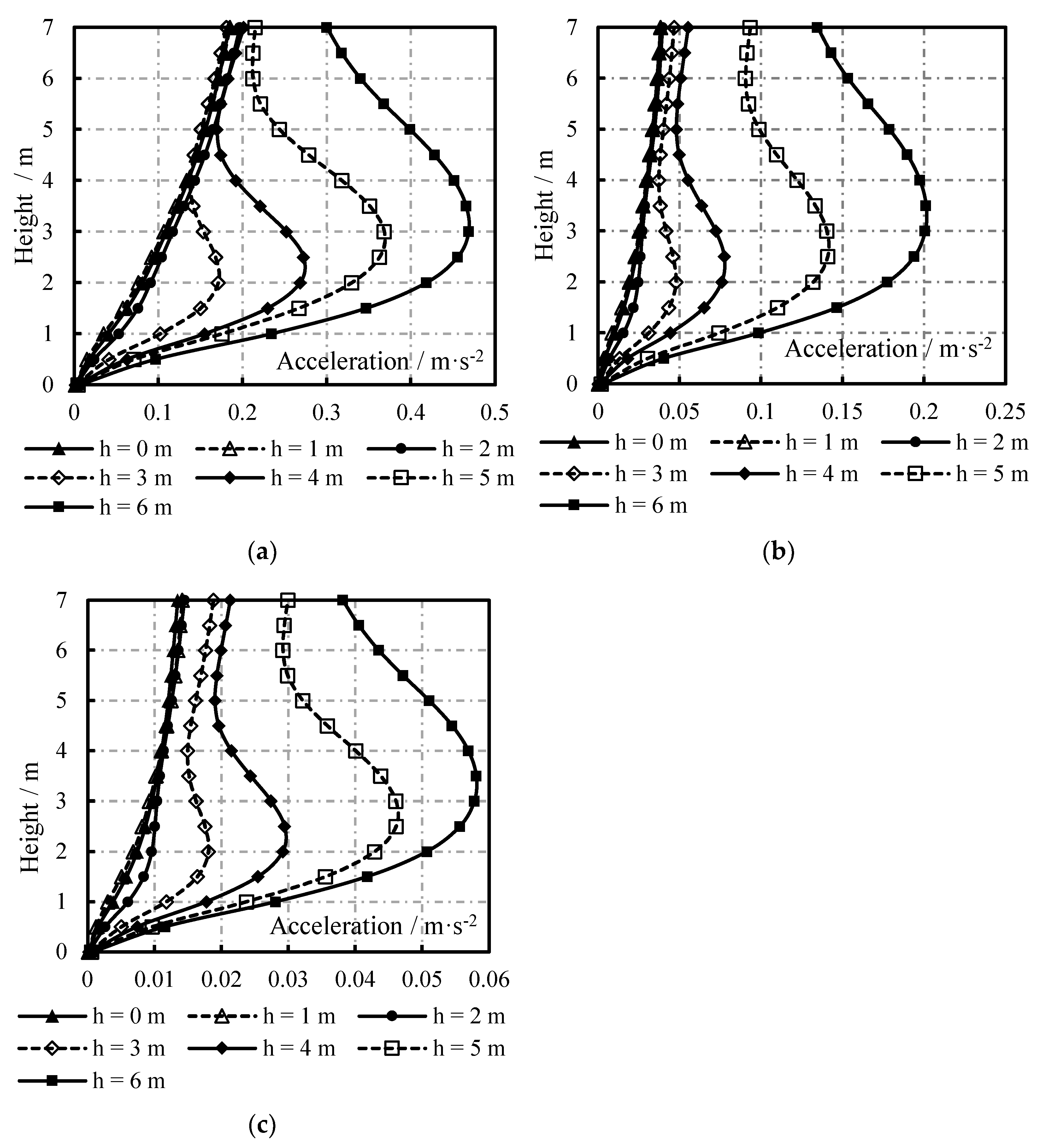
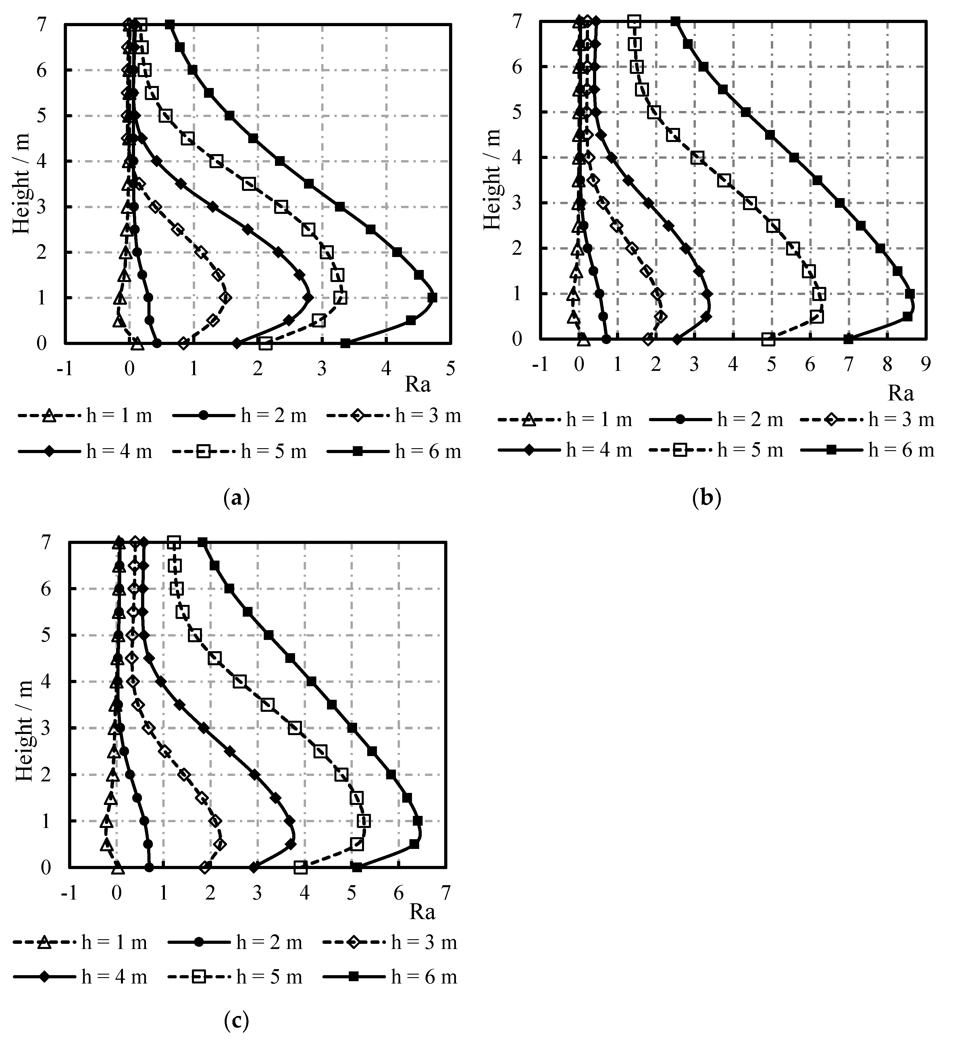
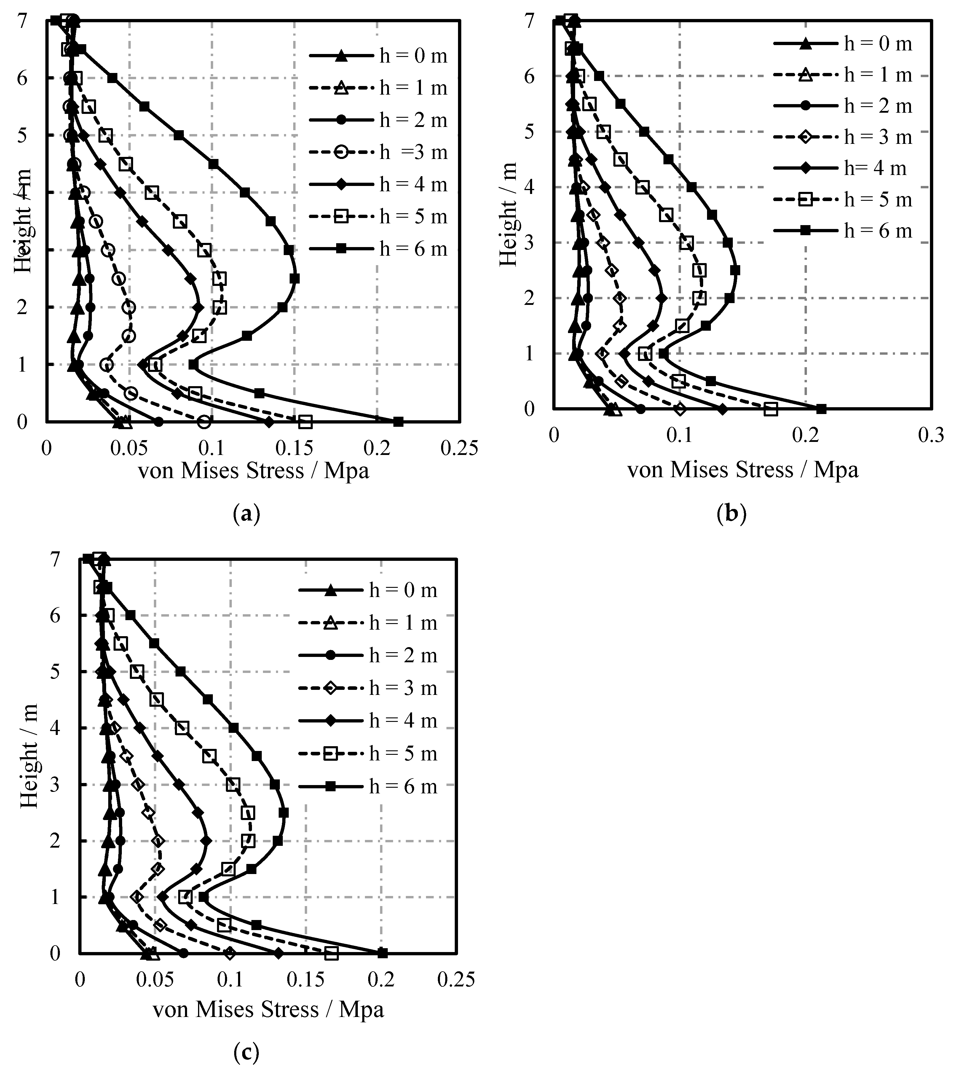
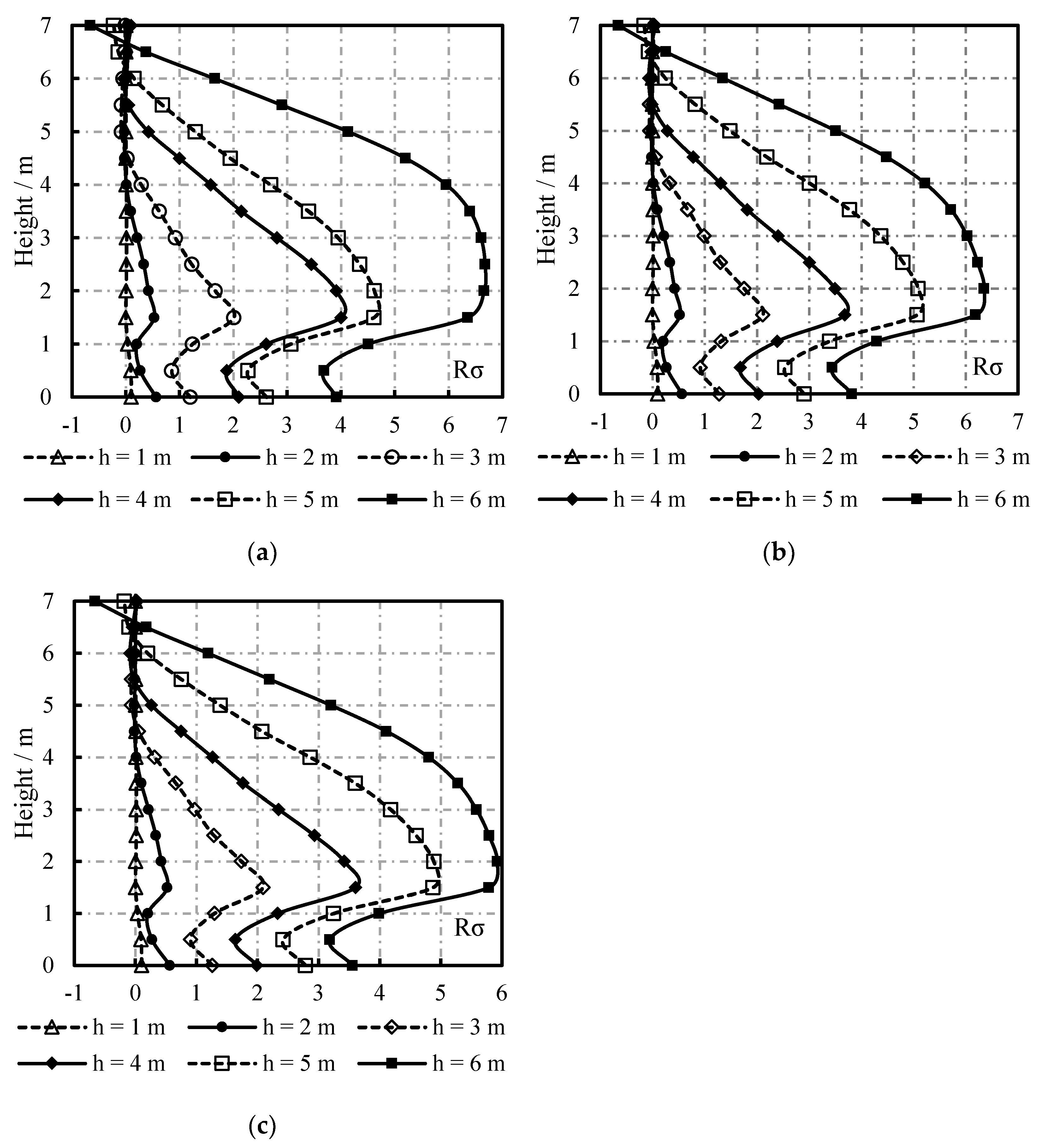
- For the cylindrical liquid-filled containers in this research, the liquid level essentially did not influence the displacement, acceleration, and stress of the liquid-filled containers under horizonal seismic action if the liquid level was low. As the liquid level rises, the displacement and acceleration of, and stress on, such liquid-filled containers increase significantly. The acceleration responses of liquid-filled containers are particularly significantly affected by the spectral characteristics of the input seismic wave.
Author Contributions
Funding
Data Availability Statement
Acknowledgments
Conflicts of Interest
References
- Ju, R.; Zeng, X. Coupled Vibration Theory of Elastic Structures and Liquids; Seismological Press: Beijing, China, 1983. (In Chinese) [Google Scholar]
- Dodge, F.T. The New Dynamic Behavior of Liquids in Moving Containers; Southwest Research Institute: San Antonio, TX, USA, 2000. [Google Scholar]
- Abramson, H.N. The Dynamic Behavior of Liquids in Moving Containers; NASA SP-106; NASA Special Publication: Washington, DC, USA, 1966. [Google Scholar]
- Ibrahim, R.A. Liquid Sloshing Dynamics: Theory and Applications; Cambridge University Press: Cambridge, UK, 2005. [Google Scholar]
- Faltinsen, O.M.; Timokha, A.N. Sloshing; Cambridge University Press: Cambridge, UK, 2009. [Google Scholar]
- Wang, J.; Li, Q.; Zhu, Z.; Lu, M.; Zhang, X. A review of numerical methods for fluid-structure interaction with large free surface sloshing. Shanghai Mech. 2001, 4, 447–454. (In Chinese) [Google Scholar]
- Wen, D.; Zheng, Z.; Sun, H. Development of aseismic research on liquid storage tanks. China Adv. Mech. 1995, 1, 60–76. (In Chinese) [Google Scholar]
- Bao, X.; Liu, J. Dynamic finite element analysis methods for liquid container considering fluid-structure interaction. Nucl. Power Eng. 2017, 38, 111–114. (In Chinese) [Google Scholar]
- Liu, J.; Bao, X.; Tan, H.; Wang, D.; Li, X. Dynamic analysis of annular liquid containers. Chin. Eng. Mech. 2018, 35, 66–73. (In Chinese) [Google Scholar]
- Xu, G.; Ren, W.; Zhang, W.; Reimerdes, H.G.; Dafnis, A.; Korsch, H. Dynamic characteristic analysis of liquid-filled tanks as a 3-d fluid-structure coupling system. China J. Mech. 2004, 3, 328–335. (In Chinese) [Google Scholar]
- Graham, E.W.; Rodriguez, A.M. The characteristics of fuel motion which affect airplane dynamics. J. Appl. Mech. 1952, 19, 381–388. [Google Scholar] [CrossRef]
- Li, Y.; Wang, J. A supplementary, exact solution of an equivalent mechanical model for a sloshing fluid in a rectangular tank. J. Fluid. Struct. 2012, 31, 147–151. [Google Scholar] [CrossRef]
- Housner, G.W. Earthquake Pressures on Fluid Containers; California Institute of Technology: Pasadena, CA, USA, 1954; pp. 1–39. [Google Scholar]
- Westergaard, H.M. Water Pressures on Dams during Earthquakes. Trans. Am. Soc. Civ. Eng. 1933, 98, 418–432. [Google Scholar] [CrossRef]
- Hall, J.F.; Chopra, A.K. Hydrodynamic effects in the dynamic response of concrete gravity dams. Earthq. Eng. Struct. Dyn. 1982, 10, 333–345. [Google Scholar] [CrossRef]
- Rajasankar, J.; Iyer, N.R.; Rao, T.V.S.R.A. A new 3-D finite element model to evaluate added mass for analysis of fluid-structure interaction problems. Int. J. Numer. Methods. Eng. 1993, 36, 997–1012. [Google Scholar] [CrossRef]
- Bao, X.; Liu, J.; Yang, Y.; Tan, H.; Wang, D. Comparative study on added mass methods for dynamic analysis of annular water tank in nuclear engineering. J. Build. Struct. 2018, 39, 130–139. (In Chinese) [Google Scholar]
- Wang, X. Finite Element Method; Tsinghua University Press: Beijing, China, 2003. (In Chinese) [Google Scholar]
- Chen, H.; Taylor, R.L. Vibration analysis of fluid-solid systems using a finite element displacement formulation. Int. J. Numer. Methods. Eng. 1990, 29, 683–698. [Google Scholar] [CrossRef]
- Everstine, G.C. Finite element formulations of structural acoustics problems. Comput. Struct. 1997, 65, 307–321. [Google Scholar] [CrossRef]
- Acoustic Analysis Guide Release 2023 R2; ANSYS, Inc.: Canonsburg, PA, USA, 2023.
- Li, Y.; Wang, Z. An Approximate Analytical Solution of Sloshing Frequencies for a Liquid in Various Shape Aqueducts. Shock Vib. 2014, 2, 118–124. [Google Scholar] [CrossRef]
- Li, Y.; Wang, Z. Unstable characteristics of two-dimensional parametric sloshing in various shape tanks: Theoretical and experimental analyses. J. Vib. Control 2016, 22, 4025–4046. [Google Scholar] [CrossRef]
- Li, Y. Fundamentals of Fluid Sloshing Dynamics; Science Press: Beijing, China, 2017. (In Chinese) [Google Scholar]

| Order | Rectangular Container Water Level h = 0.12 m | Circular Container Water Level h = 0.16 m | U-Shaped Container Water Level h = 0.115 m | ||||||
|---|---|---|---|---|---|---|---|---|---|
| Theoretical Calculation | Test | FEA | Theoretical Calculation | Test | FEA | Theoretical Calculation | Test | FEA | |
| 1 | 1.93 | 1.89 | 1.93 | 1.77 | 1.68 | 1.77 | 1.90 | 1.85 | 1.89 |
| 2 | 2.79 | 2.73 | 2.79 | 2.55 | 2.52 | 2.57 | 2.78 | 2.73 | 2.78 |
| 3 | 3.42 | 3.40 | 3.43 | 3.12 | 3.09 | 3.15 | 3.42 | 3.35 | 3.42 |
| 4 | 3.95 | 3.94 | 3.97 | 3.61 | 3.51 | 3.64 | 3.95 | 3.87 | 3.95 |
| Container | Order | |||||||||
|---|---|---|---|---|---|---|---|---|---|---|
| 1 | 2 | 3 | 4 | 5 | 6 | 7 | 8 | 9 | 10 | |
| Cuboid container (Water level h = 0.12 m) | 1.93 | 2.34 | 2.80 | 2.97 | 3.34 | 3.45 | 3.55 | 3.79 | 4.01 | 4.08 |
| Spherical container (Water level h = 0.16 m) | 1.95 | 2.57 | 2.85 | 3.04 | 3.37 | 3.44 | 3.79 | 3.80 | 3.88 | 4.12 |
| U-shaped 3D container (Water level h = 0.115 m) | 2.04 | 2.72 | 3.09 | 3.27 | 3.65 | 3.66 | 4.04 | 4.11 | 4.22 | 4.40 |
| Physical Qualities | Symbol | Value |
|---|---|---|
| Container diameter | D | 12 m |
| Container height | H | 7 m |
| Container wall thickness | t | 0.2 m |
| Liquid level | h | 6 m |
| Container elastic modulus | E | 3.10 × 10¹⁰ Pa |
| Container density | 2643 kg m−3 | |
| Container Poisson’s ratio | 0.15 | |
| Liquid density | 1000 kg m−3 | |
| Liquid acoustic velocity | c | 1435 m s−1 |
| Order | |||||
|---|---|---|---|---|---|
| 1 | 2 | 3 | 4 | 5 | |
| FEA numerical solution (rigid container) | 0.27 | 0.35 | 0.40 | 0.42 | 0.47 |
| FEA numerical solution (elastic container) | 0.27 | 0.35 | 0.40 | 0.42 | 0.47 |
| Theoretical solution | 0.27 | 0.35 | 0.40 | 0.42 | 0.47 |
| Order | Liquid Level | ||||||
|---|---|---|---|---|---|---|---|
| 0 m | 1 m | 2.0 m | 3.0 m | 4.0 m | 5.0 m | 6.0 m | |
| 1 | 19.94 | 19.94 | 19.88 | 19.45 | 18.05 | 15.93 | 13.71 |
| 2 | 20.11 | 20.11 | 20.02 | 19.48 | 18.23 | 16.30 | 14.20 |
| 3 | 26.81 | 26.81 | 26.72 | 26.13 | 24.39 | 21.46 | 18.37 |
| 4 | 29.29 | 29.28 | 29.09 | 27.85 | 24.93 | 21.88 | 19.41 |
| 5 | 38.30 | 38.30 | 38.16 | 37.10 | 34.10 | 30.44 | 26.34 |
Disclaimer/Publisher’s Note: The statements, opinions and data contained in all publications are solely those of the individual author(s) and contributor(s) and not of MDPI and/or the editor(s). MDPI and/or the editor(s) disclaim responsibility for any injury to people or property resulting from any ideas, methods, instructions or products referred to in the content. |
© 2024 by the authors. Licensee MDPI, Basel, Switzerland. This article is an open access article distributed under the terms and conditions of the Creative Commons Attribution (CC BY) license (https://creativecommons.org/licenses/by/4.0/).
Share and Cite
Fang, X.; Bao, X.; Yue, F.; Zhao, Q. A Dynamic Analysis Method of Liquid-Filled Containers Considering the Fluid–Structure Interaction. Appl. Sci. 2024, 14, 2688. https://doi.org/10.3390/app14072688
Fang X, Bao X, Yue F, Zhao Q. A Dynamic Analysis Method of Liquid-Filled Containers Considering the Fluid–Structure Interaction. Applied Sciences. 2024; 14(7):2688. https://doi.org/10.3390/app14072688
Chicago/Turabian StyleFang, Xibing, Xin Bao, Fengjiang Yue, and Qiyuan Zhao. 2024. "A Dynamic Analysis Method of Liquid-Filled Containers Considering the Fluid–Structure Interaction" Applied Sciences 14, no. 7: 2688. https://doi.org/10.3390/app14072688
APA StyleFang, X., Bao, X., Yue, F., & Zhao, Q. (2024). A Dynamic Analysis Method of Liquid-Filled Containers Considering the Fluid–Structure Interaction. Applied Sciences, 14(7), 2688. https://doi.org/10.3390/app14072688