A Novel Physics-Guided Neural Network for Predicting Fatigue Life of Materials

Abstract

A physics-guided neural network (PGNN) is proposed to predict the fatigue life of materials. In order to reduce the complexity of fatigue life prediction and reduce the data required for network training, the PGNN only predicts the fatigue performance parameters under a specific loading environment, and calculates the fatigue life by substituting the load into the fatigue performance parameters. The advantage of this is that the network does not need to evaluate the effect of numerical changes in the load on fatigue life. The load only needs to participate in the error verification, which reduces the dimension of the function that the neural network needs to approximate. The performance of the PGNN is verified using published data. Due to the reduction in the complexity of the problem, the PGNN can use fewer training samples to obtain more accurate fatigue life prediction results and has a certain extrapolation ability for the changes in trained loading environment parameters. The prediction process of the PGNN for fatigue life is not completely a black box, and the prediction results are helpful for scholars to further study the fatigue phenomenon.

1. Introduction

The fatigue failure of materials has always been the focus of research in the field of engineering. Fatigue failure is sudden and destructive. Unlike static failure, it may occur when its actual load is much lower than its yield load. In order to achieve a balance between safety and economy, it is necessary to predict the fatigue life of materials in the engineering field.

In Europe, research on fatigue began in the early 19th century. German mining engineer Wilhelm Albert was the first to observe that the strength of metal materials operating under repeated loading is lower than the static strength of the materials. In 1854, Braithwaite was the first to coin the term “fatigue” to describe the phenomenon of metal cracking under repeated action at lower loads [1]. Many researchers have since studied fatigue in terms of the stress amplitude–life curve (Albert Wohler), the influence of average stress on fatigue life (Gerber, Goodman, Soderberg) [2,3,4], and Basquin’s equation (Basquin) [5]. These efforts have promoted the development of fatigue research.

The traditional method for fatigue life prediction is the explicit method. One of the typical examples is the Basquin equation, which characterizes the relationship between fatigue life and load. Using the Basquin equation, only two fatigue performance parameters need to be determined to directly determine the fatigue life in combination with the load. However, it has the following limitations: 1. There are many factors that affect the fatigue life of materials, such as temperature, notch, corrosion, stress ratio, etc. These changes in the service environment will directly affect the correspondence between load and fatigue life. 2. The two fatigue performance parameters need to be obtained by the corresponding fatigue test, and the obtained parameters can only be used in the load environment corresponding to the fatigue test, which has high requirements for time and economic resources. Based on the above reasons, the traditional explicit model cannot meet the needs of the engineering field.

Due to the rapid development of computer technology, machine learning technology has gradually played a very important role in the engineering field [6]. It is difficult to determine the fatigue life directly by the determined mathematical solution method, and the fatigue experiment usually has noise [7,8,9]. There may be errors in the measurement of experimental parameters [10]. Machine learning is a promising solution for similar fields. At present, there are many machine learning methods used in the prediction of fatigue life: Liu et al. used the random forest method to predict the fatigue life of rubber under constant amplitude strain loads [11]. Bao et al. predicted the fatigue life of laser cladding Ti-6Al-4V alloys using the support vector regression method [12]. Yang et al. successfully predicted the multiaxial fatigue life with different loading paths through a recurrent neural network [13]. Among them, the neural network method has been widely used in the field of fatigue life prediction due to its structural diversity. As a fully data-driven model [14], the above machine learning methods rely heavily on a sufficient number of training data [15], and the data extrapolation ability is poor [16]. Especially when the coverage of training samples is insufficient, its predictive ability will be greatly reduced [17].

Based on the above reasons, some scholars have tried to embed information into neural networks to improve their data extrapolation capabilities. RASSI et al. embedded the Stokes equation into the loss function of the neural network to predict the pressure, velocity and other parameters inside the fluid. In the process of learning, the network not only satisfies the error reduction of the training data, but also ensures that the prediction results conform to the Stokes equation [18]. In the field of fatigue life prediction, Chen et al. proposed a physical probability-guided neural network. Through a specially designed neural network structure and constraints on the bias and weight range of some neurons, the fatigue life prediction results conform to the characteristics of the S-N curve and can also output its predicted confidence interval [19]. Viana et al. proposed a hybrid neural network, which successfully predicted the fatigue life of the main bearing of the wind turbine through the empirical formula of bearing life combined with the recurrent neural network [20,21,22].

The machine learning methods mentioned above are all direct predictions of the fatigue life of materials, some of which add some constraints to make the prediction results conform to the S-N curve characteristics or other natural facts. This study proposes a physics-guided neural network (PGNN) for predicting fatigue life. Different from the above published methods, the load and fatigue life of the material under the same loading environment follow a certain power–law relationship, that is, the Basquin equation. Instead of directly predicting the fatigue life of the material, the neural network predicts the fatigue life parameters under the corresponding loading environment, and the corresponding fatigue life is determined by the fatigue life parameters combined with the loading stress. The proposed method does not consider the influence of the numerical change of the load on the fatigue life, so the load does not participate in the parameter update of the neural network, which simplifies the dimension of the function that the neural network needs to approximate. The simplification of the process means that the number of training data required can be effectively reduced. The ratio of the number of training samples to the number of validation samples used in this study was 1:3 (the number of training samples was 26, and the number of validation samples was 78) to verify the model’s ability to predict fatigue life under different loading environments (such as notch and stress ratio). Due to the randomness of the training path of the neural network, the prediction result is the optimal result after repeated training for 5 times [23].

The remainder of this paper is organized as follows. Section 2 details the physical model and the operating mechanism of the proposed PGNN. In Section 3, the collected experimental data are used to verify the predictive ability of the PGNN. Section 4 presents the conclusions drawn from the study.

2. Materials and Methods

The proposed (PGNN) consists of empirical formulas and data-driven neural networks, which are briefly described below.

2.1. Empirical Model

The traditional life prediction model is an explicit model, which has the advantage of a simple structure. For example, in 1910, Basquin [6] proposed the following power–law expression describing load and fatigue life:

$$\sigma ={\sigma }_f^{\prime }{\left(N_f\right)}^b$$

(1)

where σ represents the stress level under the loading cycle of the material, $N_f$ is the fatigue life, and ${\sigma }_f^{\prime }$, $b$ represents the fatigue constant under a given load.

Formula (1) shows that under a certain loading environment (temperature, corrosion, stress concentration factor, etc.), the fatigue life of the material is a certain power function relationship with its actual load. The fatigue performance constant (${\sigma }_f^{\prime }$, $b$) characterizes its specific loading environment, that is, all loading environments can be determined by two fatigue performance parameters, ${\sigma }_f^{\prime }$ and $b$. Therefore, it is feasible to establish a model with loading environment parameters as input and fatigue parameters (${\sigma }_f^{\prime }$, $b$) as output to predict the fatigue life of materials under different loading conditions.

In 1914, Stromeyer [24] proposed the following expression based on the Basquin formula:

$$(\sigma -{\sigma }_f)={\sigma }_f^{\prime }{\left(N_f\right)}^b$$

(2)

In this expression, ${\sigma }_f$ characterizes the fatigue limit of the material.

Formula (2) introduces the fatigue limit of the material on the basis of the Basquin equation. However, the new parameter has limited improvement in the accuracy of fatigue life prediction. The smaller the number of parameters to be determined, the more conducive to the convergence of the model. Based on the above reasons, this study uses Formula (1) to establish a fatigue life prediction model.

In order to calculate the fatigue life conveniently, Formula (1) is rewritten as follows:

$$N_f={(\frac{\sigma }{{\sigma }_f^{\prime }})}^{\frac{1}{b}}$$

(3)

The range of common fatigue cycle life values can be distributed between 1 × 10² and 1 × 10⁸. Parameters of such an order of magnitude cannot be calculated in a neural network that relies on gradient update. The commonly used method is to change the fatigue life and load into a logarithmic form:

$$\log N_f=\left(\frac{1}{b}\right)\left(\log {\sigma }_{max}-\log {\sigma }_f^{\prime }\right)$$

(4)

The fatigue performance parameters ${\sigma }_f^{\prime }$ and $b$ can be obtained from the fatigue test results, and the fatigue life of any load value under the corresponding loading environment can be estimated.

2.2. The Structure of the Proposed Method

2.2.1. Introduction of Artificial Neural Network

An artificial neural network is a mathematical model similar to the structure of brain synaptic connections to process information. Similar to brain cells, an ANN consists of a large number of processing units called neurons. The most widely used ANN is back the propagation neural network (BPNN) [6]. The BPNN is a multi-layer, supervised, feedforward network using back propagation rules. The BPNN can learn and store a large number of input–output mode mapping relationships without revealing the mathematical equations describing this mapping relationship in advance. Its learning rule is to use the steepest descent method to continuously adjust the weight and bias of network neurons through back propagation, so as to minimize the error of the network. Its main feature is that the signal is forward propagation, and the error is back propagation.

2.2.2. Structure of PGNN

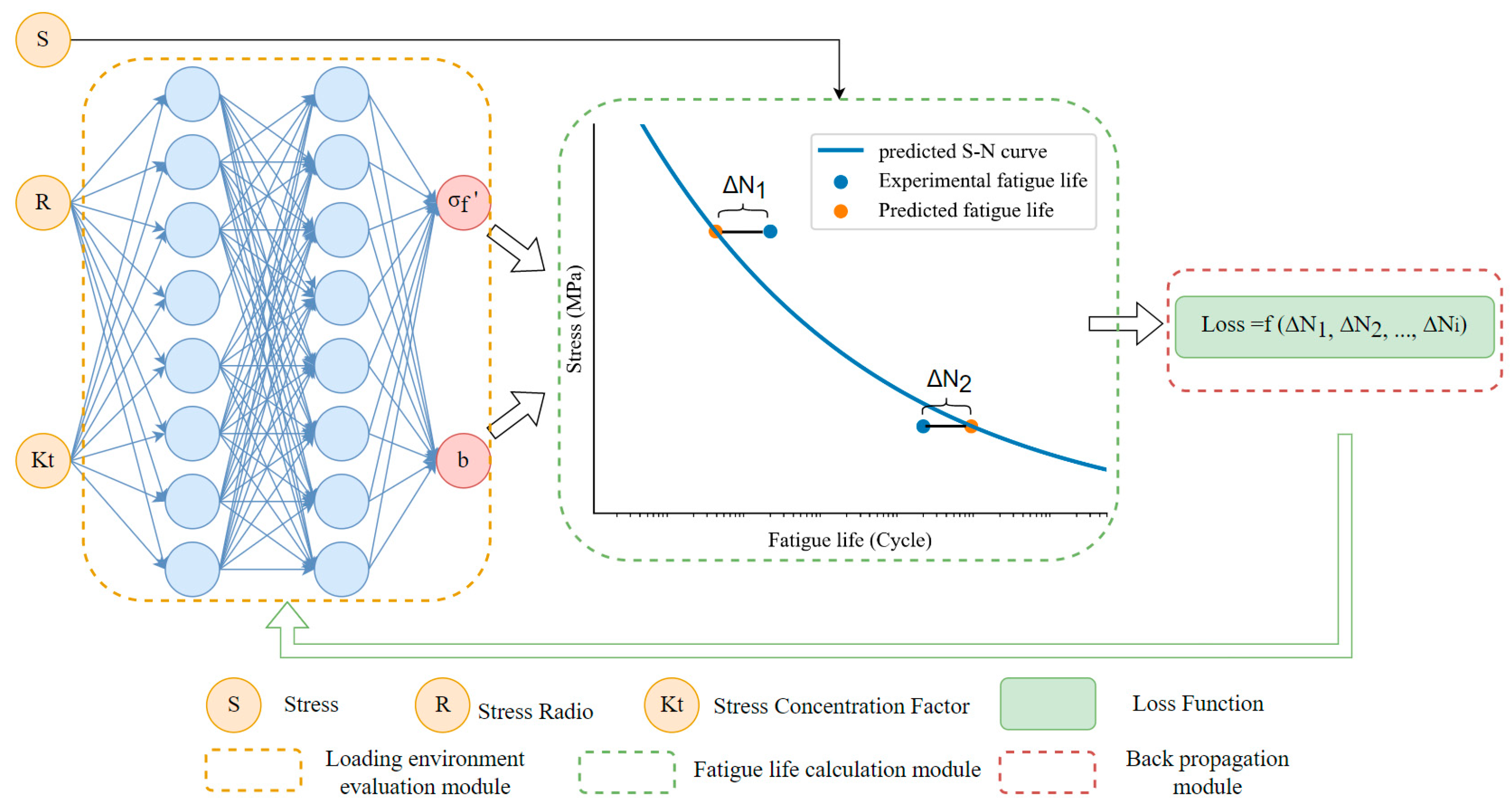
The PGNN consists of three modules, which are the evaluation module of the loading environment, the fatigue life calculation module and the back propagation module. Its structure is shown in Figure 1.

The loading environment evaluation module consists of a four-layer fully connected neural network. The input is the loading environment parameters. In this study, the loading environment parameters include the stress ratio (R) and stress concentration factor (Kt) caused by the notch, and the output is the fatigue parameter ${\sigma }_f^{\prime }$, $b$ of the Basquin formula. The purpose is to construct the S-N curve corresponding to the loading environment parameters.

The core of the fatigue life calculation module is the Basquin equation. Its input is the load S, and the fatigue parameter ${\sigma }_f^{\prime }$, $b$ obtained by the loading environment evaluation module, where the load S is the maximum stress ${\sigma }_{max}$. The output is fatigue life, where $∆N_i$ is the difference between the actual fatigue life $N_E$ and the predicted fatigue life $N_P$ of the ith sample ($N_E-N_P$).

The core of the back propagation module is the loss equation. The fatigue life difference $(N_E-N_P$) obtained by the fatigue life calculation module is used as the input, and the loss equation is constructed to quantify the gap between the predicted target and the actual value. After the loss function value is obtained, the gradient of all neurons is calculated and back propagated to the loading environment assessment module to complete the parameter update of the neurons in the environment assessment module.

The overall PGNN operation process is as follows: the fatigue parameter ${\sigma }_f^{\prime }$,$b$ is calculated by a fully data-driven loading environment evaluation module. Then, the fatigue life calculation module guides the network to obtain the corresponding fatigue life. The back propagation module calculates the loss function and reverses the conduction gradient with the goal of minimizing the loss value.

For the first time, the fatigue parameter ${\sigma }_f^{\prime }$,$b$ obtained by inputting the loading environment parameters (R, Kt) into the network is a low-fidelity fatigue parameter. The fatigue parameter ${\sigma }_f^{\prime }$,$b$ is corrected by the high-fidelity experimental load S and the experimental fatigue life $N_E$ to obtain a higher-fidelity fatigue parameter ${\sigma }_f^{\prime }$,$b$. Then, the fatigue life values of high fidelity under various loading environments can be obtained.

2.2.3. Loss Function

The loss function can quantify the gap between the predicted value and the actual value of the predicted target and guide the update of the network parameters. After the network obtains the loss value, the gradient of all the updateable parameters of the network is calculated with the goal of minimizing the loss value. The calculated gradient is back propagated to the corresponding parameters to complete the update of the parameters to achieve the purpose of minimizing the loss function.

Usually, the non-negative number is selected as the loss, and the smaller the value is, the more accurate the prediction is, and the loss in perfect prediction is 0. At present, the loss function commonly used in regression problems is the mean square error function, and its total error performance function is as follows:

$$\mathrm{L}\mathrm{o}\mathrm{s}\mathrm{s}=\frac{1}{n}\sum _{i=1}^n{{(N}_P-N_E)}^2$$

(5)

where $N_P$ is the predicted logarithmic cycle life, $N_E$ is the experimental logarithmic cycle life, and n is the predicted total number of samples.

2.3. Models Involved in Comparative Verification

In order to verify the performance of the proposed method, the traditional artificial neural network (ANN) and support vector regression (SVR) methods are introduced to compare the same training samples. The SVR method is briefly introduced here.

Support vector regression (SVR) is a variant of the support vector machine (SVM) used in regression tasks. The principle is to generate a hyperplane from its kernel function, so that the hyperplane is close enough to all samples to achieve the purpose of regression. Radial basis function (RBF) is widely used in SVR, and C and gamma are two hyperparameters that affect its performance, where C is the penalty coefficient, which affects the degree of fitting and generalization of the model to the sample. Gamma represents the influence range of a single sample on the whole set of samples. In this study, the values of C and gamma were determined by orthogonal experiments, where C was set to 35 and gamma was set to 0.16.

The SVR model was established based on the Scikit-learn machine learning website [25], and the proposed PGNN and ANN are based on the Pytorch deep learning framework [26]. The SVR method has a certain prediction result for the same training sample after training when the kernel function is constant, and the neural network may be uncertain even for the same training set after training due to the random initialization of the internal neurons. Therefore, this study uses the method of repeating training 5 times to obtain the best value for the proposed PGNN and ANN. 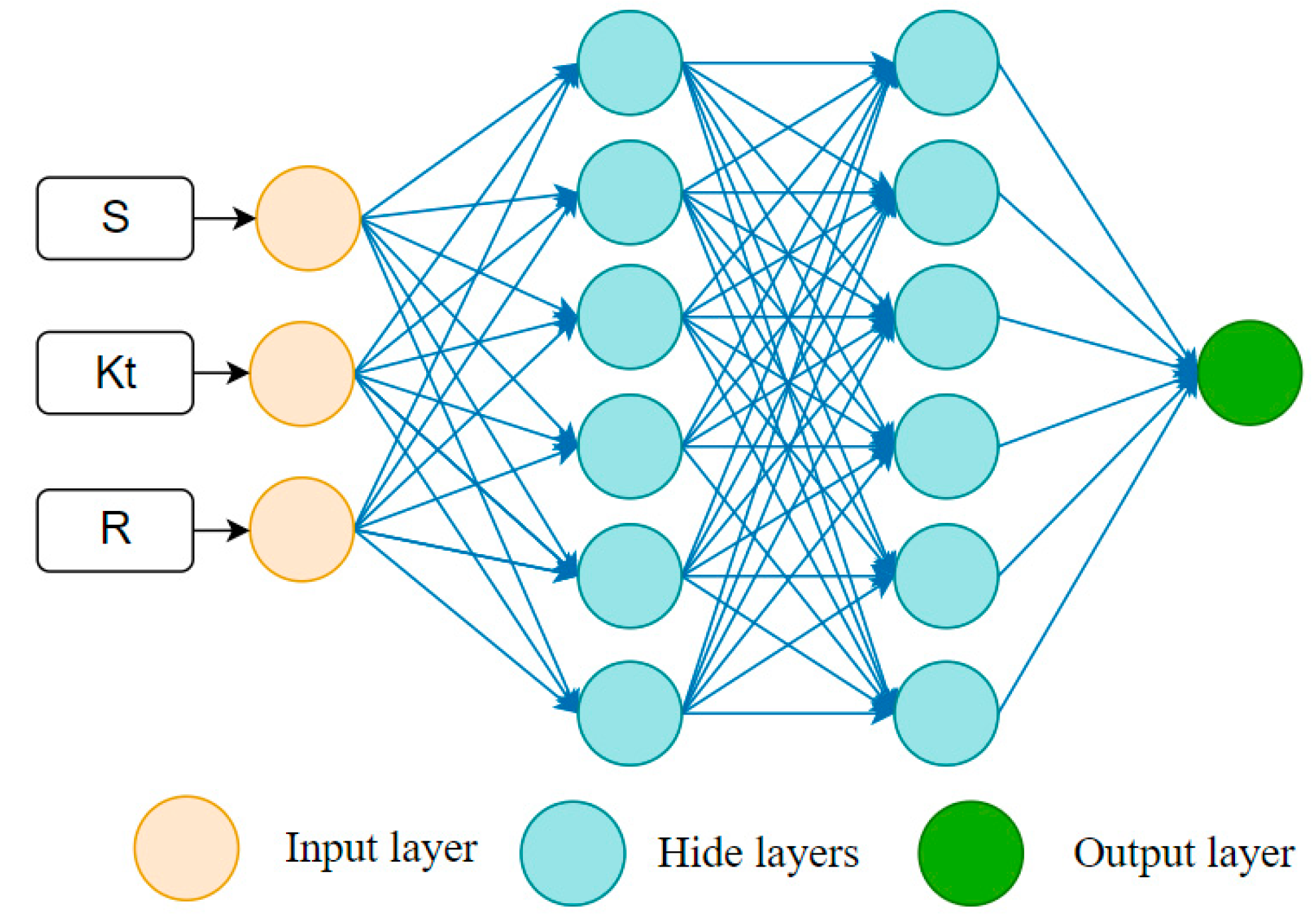The structure of the PGNN is Figure 1, and the ANN participating in the comparison test is a fully connected neural network with 4 layers. The inputs of ANN and SVR are load S, stress concentration factor Kt and stress ratio R, and the output is logarithmic fatigue life. The structure of ANN is shown in Figure 2.

The batch size, number of Epochs, learning rate and activation function affect the convergence ability of the neural network. The same hyperparameters are set for both the PGNN and ANN, as shown in

Table 1. The hyperparameters of SVR, PGNN and ANN.

Hyperparameters	SVR	PGNN	ANN
Penalty coefficient	35	—	—
The influence domain of a single vector	0.16	—	—
Batch size	—	5	5
Number of epochs	—	2000	2000
Learning rate	—	0.001	0.001
Activation function	—	ReLU	ReLU

.

2.4. Data Used to Verify the Model

This study used the fatigue data of 2024-T4 aluminum alloys in the Metal Material Performance Development and Standardization Manual (MMPDS) [27] to verify the predictive ability of each model. The aluminum alloy sample is a V-notched bar. Different sizes of the notch produce different sizes of stress concentration factor Kt, and different sizes of the stress ratio (R) are used for fatigue test loading. Detail dimensions of the specimen are shown in

Table 2. Detail dimensions of the specimen.

Kt	Gross Diameter/mm	Net Diameter/mm	Notch Root Dadius/mm	Flanj Angle/°
1.6	11.43	10.16	2.54	60
2.4	12.70	10.16	0.81	60
3.4	11.43	10.16	0.25	60

. The numbers of the samples are shown in

Table 3. Numbers of the samples.

Stress Concentration Factor (Kt)	Stress Ratio (R)	Numbers of Samples
1.6	−1, −0.37, 0.06, 0.46	37
2.4	−1, −0.37, 0.06, 0.46, 0.74	33
3.4	−1, −0.37, 0.06, 0.46, 0.74	53

.

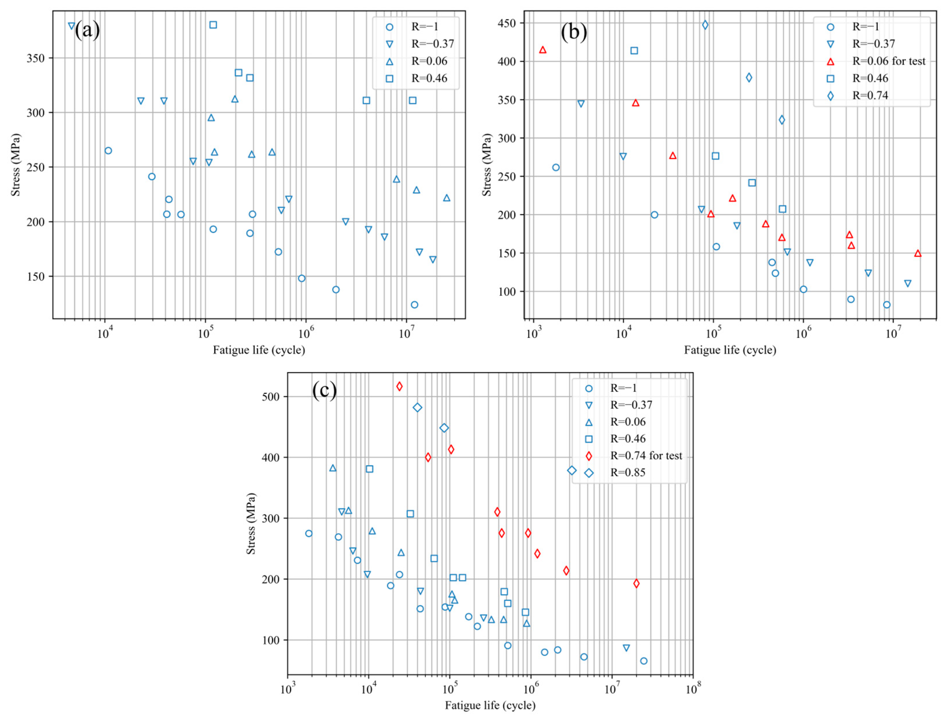
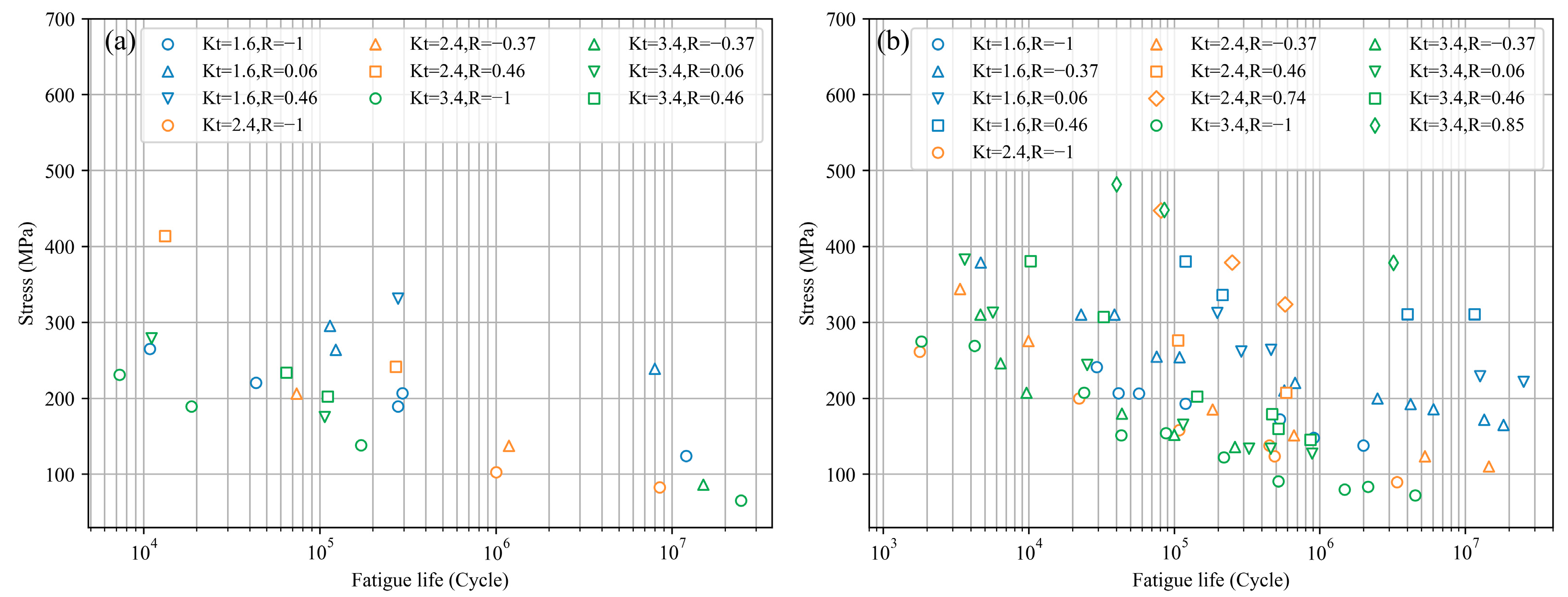
Two sample sets (Kt = 2.4, R = 0.06) and (Kt = 3.4, R = 0.74) are taken as test samples. The test samples do not participate in the subsequent training to verify the extrapolation performance of the PGNN. In order to verify the predictive ability of the model in small training samples, the remaining samples are divided into four groups in a similar form to K-fold cross-validation. Each case takes one group as the training sample and the remaining three groups as the verification sample. Therefore, there are four cases in total. The training samples in each case account for 25%, and the verification samples account for 75%. The verification samples do not participate in the training and are used to evaluate the prediction ability of the model. All samples are shown in Figure 3.

3. Results and Discussions

The accuracy of the prediction results can be measured using the root mean square error (RMSE) function as follows:

$$\mathrm{R}\mathrm{M}\mathrm{S}\mathrm{E}=\sqrt{\frac{1}{n}\sum _{i=1}^n{(\log N_i^p-\log N_i^e)}^2}$$

(6)

where n is the total number of samples, $N_i^p$ and $N_i^e$ are the life prediction value and experimental test value of the ith sample, respectively.

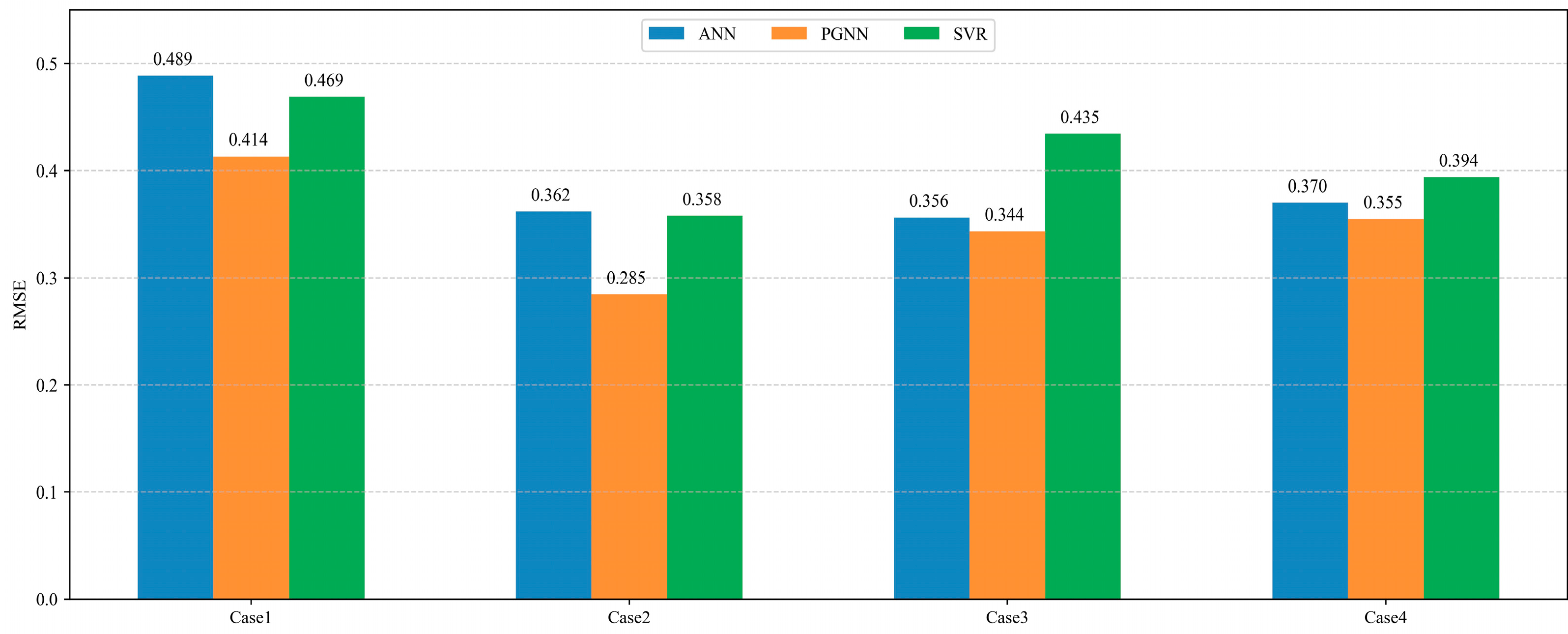
Figure 4 shows the fatigue life prediction RMSE of the ANN, PGNN and SVR in all four cases. It can be seen that the ANN, PGNN and SVR achieved the highest prediction error in Case 1, while the three methods achieved the lowest prediction error in Case 2. The average prediction error of Case 3 and Case 4 is relatively close. It shows that the selection of training samples has a non-negligible impact on the prediction accuracy of the model. One way to solve this problem is to carefully select training samples. The selected training samples should be able to cover a sufficient range. The noise of the samples is small and the samples should be representative. On the other hand, it is also necessary to integrate the ML model with specific prior knowledge to constrain or guide the prediction results of the model, so that its prediction ability is less affected by the randomness of training sample selection, which will make the prediction results of the model more credible under the condition of limited sample size.

In all cases, the RMSE of the predicted results of the PGNN is the smallest, indicating that the PGNN has an advantage in the accuracy of fatigue life prediction compared with the ANN and SVR. The following is a further analysis of Case 2, in which all three models achieved the minimum error.

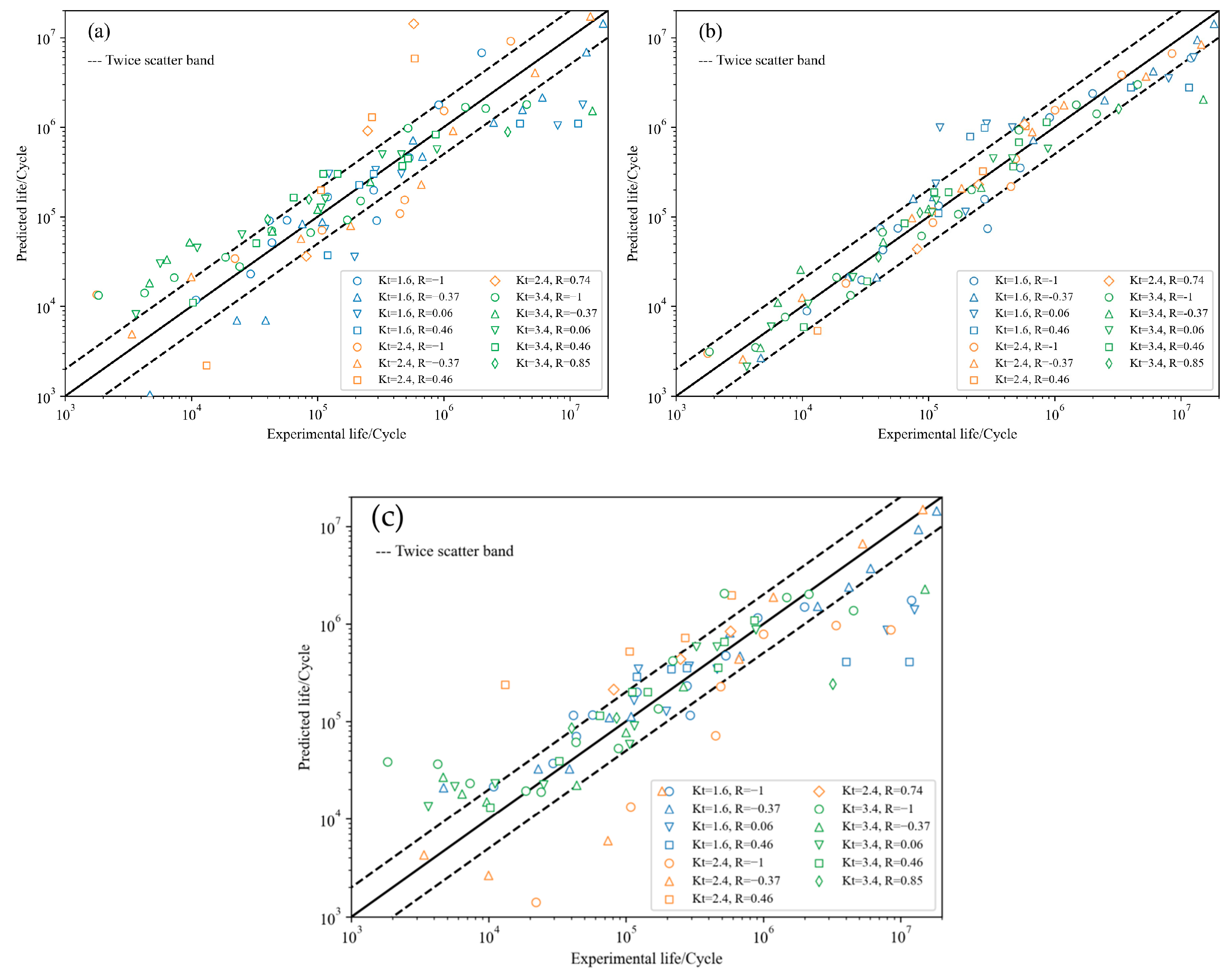
Figure 5 shows the details of the training samples and validation samples in Case 2, and Figure 6 shows the fatigue life prediction results of the ANN, PGNN and SVR for Case 2.

The error line in Figure 6 is a double error line. Among them, the ANN and SVR have higher fatigue life prediction results than the double error line, while the PGNN has lower fatigue prediction results than the double error. This is consistent with the RMSE results in Figure 4, indicating that the PGNN has higher accuracy in predicting the fatigue life of Case 2 in this study.

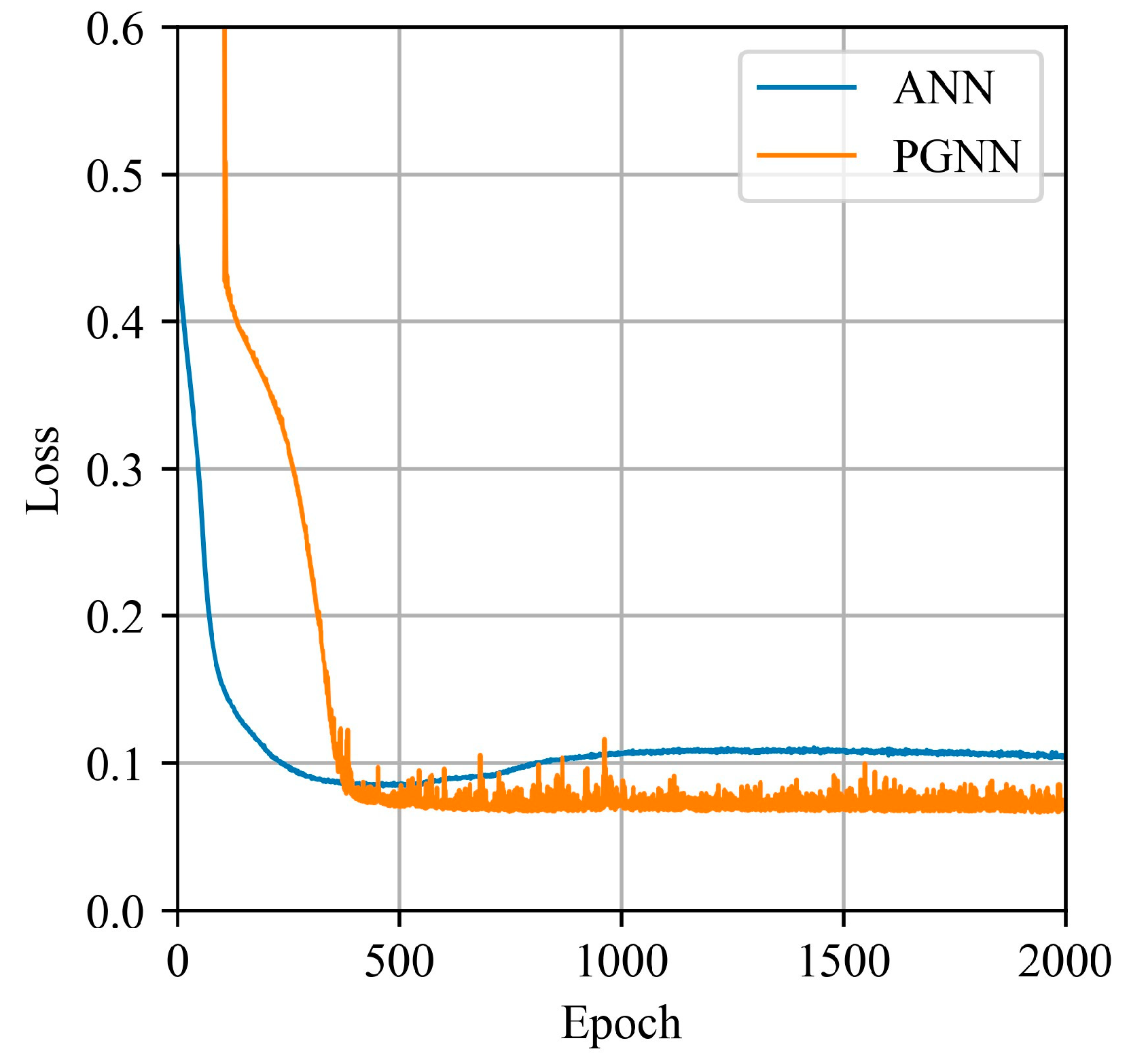
After each epoch, the ANN and PGNN calculate the loss function for all samples in Case 2 to determine the progress of network training. Figure 7 shows the loss function iteration process of ANN and PGNN. The value of the loss function of ANN is reduced to the minimum value, and the loss function increases with the continuous training, indicating that the prediction error of ANN in Case 2 increases with the continuous training. It shows that the ANN has the phenomenon of over-fitting training samples. The loss function of the PGNN tends to be stable after falling to the minimum value, indicating that the PGNN can effectively resist the over-fitting of training samples.

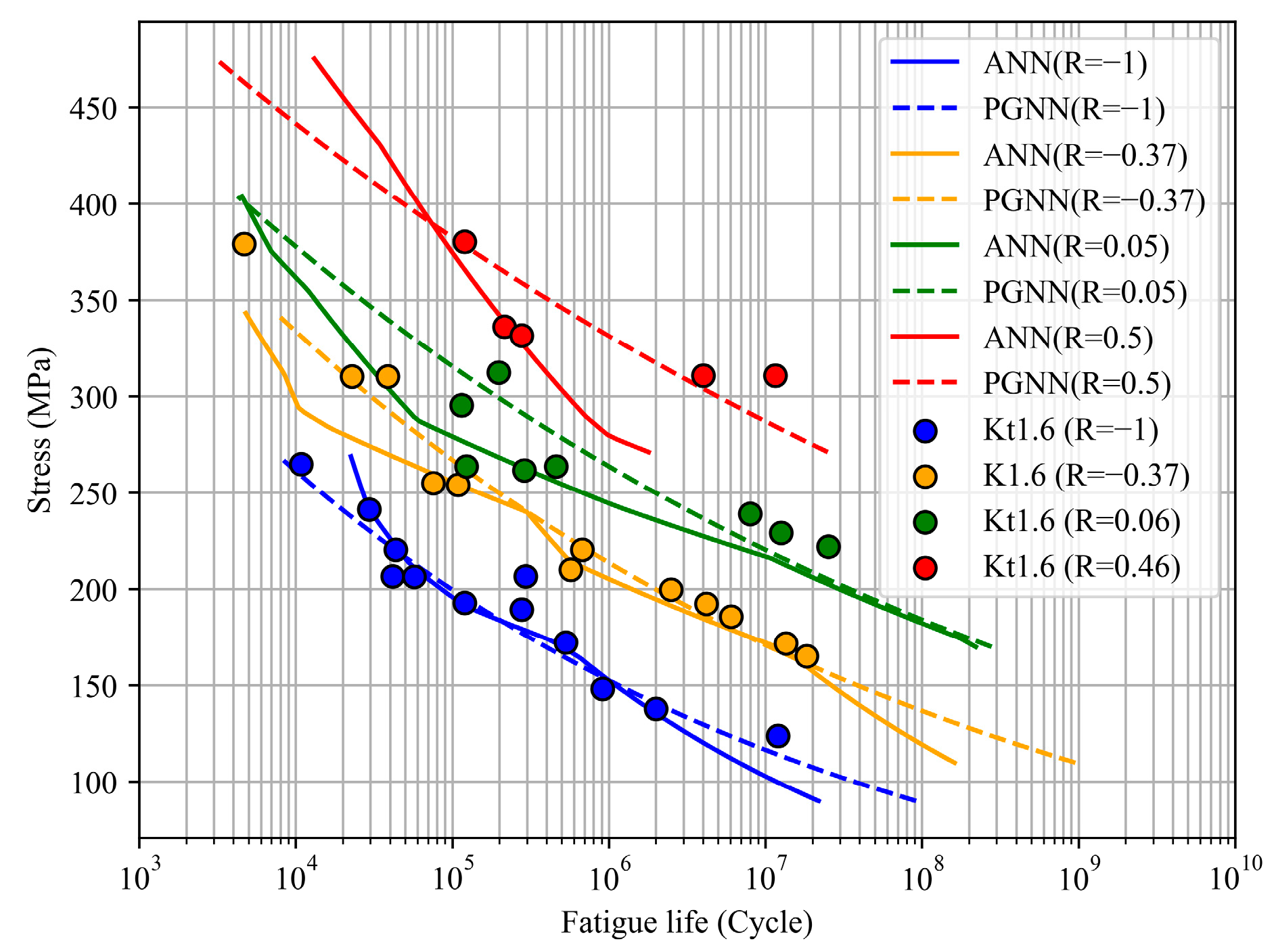
After training, the ML method can output the fatigue life prediction results of any load under certain conditions. Figure 8 shows the S-N curves of each stress ratio R output by the ANN and PGNN under the condition of Kt = 1.6. Among them, the S-N curves output by the PGNN are all smooth curves, while the S-N curves output by ANN, as a purely data-driven method, are irregular line segments. In Figure 8, the S-N curve output by the ANN has a sudden increase in the slope, which is inconsistent with reality.

In fact, the S-N curve output by the PGNN is determined by the fatigue parameter ${\sigma }_f^{\prime }$,$b$ corresponding to the specific loading environment, which is certainly a smooth power function curve. Table 3 gives the predicted values of the fatigue parameters ${\sigma }_f^{\prime }$,$b$ for all the stress concentration factors Kt and the stress ratio R involved in the sample for the PGNN trained in Case 2.

The predicted values of fatigue parameters in

Table 4. The predicted value of ${\sigma }_f^{\prime }$,$b$ outputted by PGNN.

Fatigue Performance Parameters	Kt = 1.6 (Stress Concentration Factor)		Kt = 2.4 (Stress Concentration Factor)		Kt = 3.4 (Stress Concentration Factor)
	$${\mathit{\sigma }}_{\mathit{f}}^{\mathbf{\prime }}$$	$$\mathit{b}$$	$${\mathit{\sigma }}_{\mathit{f}}^{\mathbf{\prime }}$$	$$\mathit{b}$$	$${\mathit{\sigma }}_{\mathit{f}}^{\mathbf{\prime }}$$	$$\mathit{b}$$
(Stress ratio) R = −1	2.885	−0.117	2.938	−0.150	3.120	−0.195
(Stress ratio) R = −0.37	2.911	−0.097	3.017	−0.141	3.201	−0.200
(Stress ratio) R = 0.06	2.889	−0.078	3.054	−0.137	3.237	−0.197
(Stress ratio) R = 0.46	2.894	−0.062	3.107	−0.132	3.271	−0.183
(Stress ratio) R = 0.74	—	—	3.120	−0.101	3.260	−0.143
(Stress ratio) R = 0.85	—	—	—	—	2.972	−0.063

can be used to further analyze the influence of loading environment on the change trend of fatigue life. This advantage of the machine learning method can provide help for scholars to study the fatigue phenomenon without carrying out a significant amount of fatigue experiments, saving time and resources.

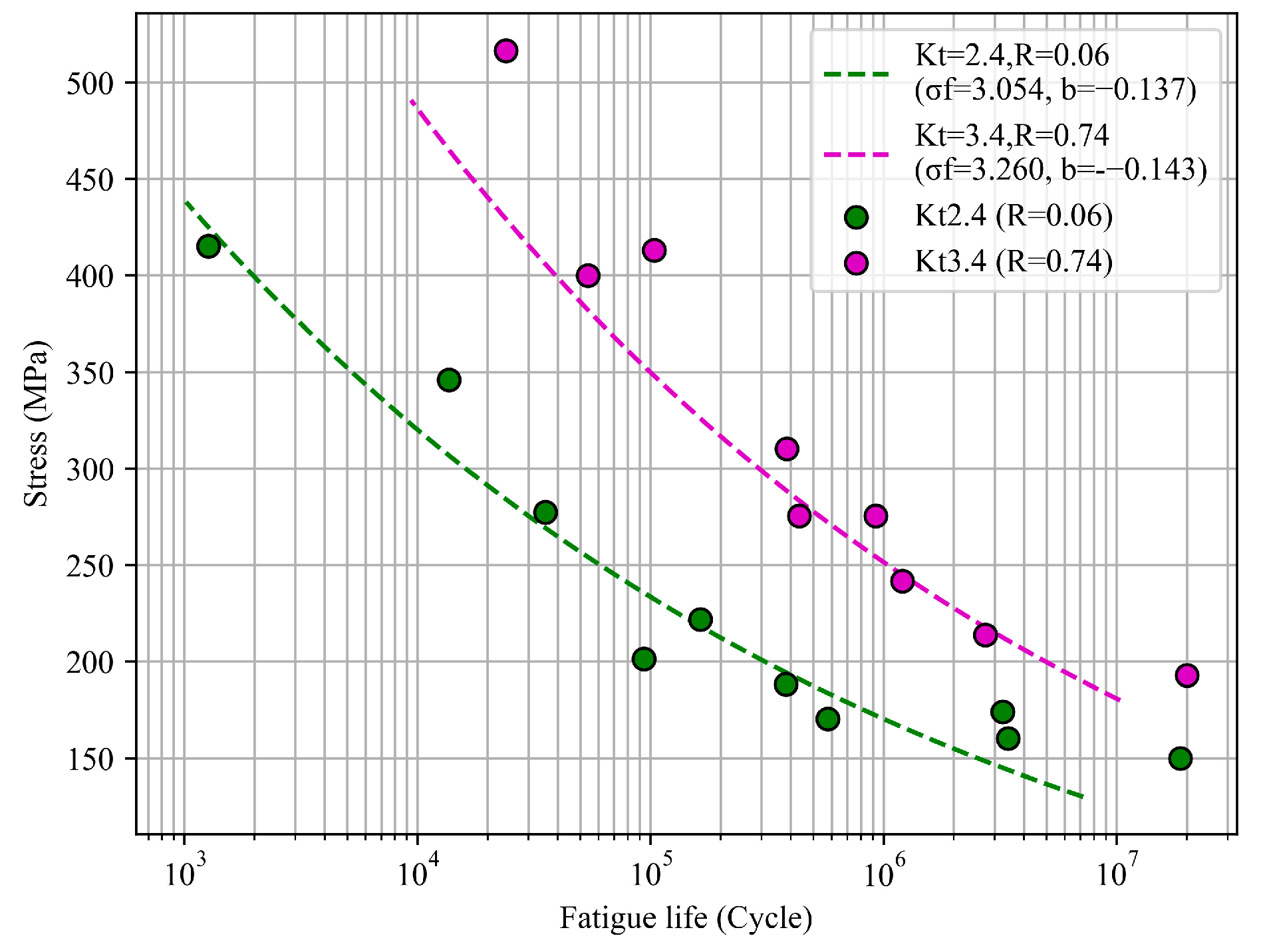
The sample set (Kt = 2.4, R = 0.06) and (Kt = 3.4, R = 0.74) are used as test samples to verify the data extrapolation ability of the PGNN method. Figure 9 shows the S-N curve of the test sample set generated by the PGNN.

According to Figure 9, for the two test sample sets (Kt = 2.4, R = 0.06) and (Kt = 3.4, R = 0.74), the PGNN successfully predicted the corresponding S-N curve. It shows that the PGNN has a certain data extrapolation ability.

It is worth mentioning that the data extrapolation ability of the PGNN proposed in this study is limited to the range of environmental factors that have been trained. In this study, it is the stress ratio and stress concentration factor. The addition of new environmental parameters such as temperature will lead to the retraining of the network, and all samples in the training set should contain temperature parameters. All environmental parameters must also adopt a unified unit of measurement. Therefore, this method can be used as a data extrapolation tool for fatigue tests, and environmental factors that are not included in fatigue tests cannot be evaluated.

4. Conclusions

This study proposes a physics-guided neural network for predicting the fatigue life of materials. Taking the loading environment parameters as the output, the parameters of the S-N curve corresponding to the loading environment are predicted instead of directly predicting the fatigue life, which greatly simplifies the prediction process of fatigue life. The predicted fatigue performance parameters can help further research on fatigue phenomena. The proposed method can obtain more accurate fatigue life prediction results based on smaller training samples, and has a certain data extrapolation ability. The main conclusions are as follows:

• According to the characteristics of the power–law relationship between fatigue life and load, predicting the S-N curve instead of directly predicting the fatigue life can simplify the fatigue life prediction process. This study can provide a reference for the prediction of fatigue life by machine learning methods in the future.
• Predicting the S-N curve under a specific loading environment means that the model is not completely a black box for the prediction process of fatigue life under corresponding conditions, which is helpful for the community to further study the fatigue phenomenon.
• The prediction accuracy of machine learning methods is more dependent on the selection of training samples. The prediction results of the models obtained by selecting different training samples are different.

Machine learning methods have shown great potential in the field of fatigue life prediction. In order to obtain more reliable prediction results, on the one hand, more complex models can be studied, and on the other hand, it is necessary to simplify the research problems. In addition, the influence of the randomness of training samples on the prediction accuracy of the model should also be paid attention to. Only in the ideal case are the training samples sufficient and in many cases, only a limited number of training samples are available. The ideal model should be able to reduce the randomness caused by small batches of samples, which can make the prediction results more reliable.