U-ETMVSNet: Uncertainty-Epipolar Transformer Multi-View Stereo Network for Object Stereo Reconstruction

Abstract

The Multi-View Stereo model (MVS), which utilizes 2D images from multiple perspectives for 3D reconstruction, is a crucial technique in the field of 3D vision. To address the poor correlation between 2D features and 3D space in existing MVS models, as well as the high sampling rate required for static sampling, we proposeU-ETMVSNet in this paper. Initially, we employ an integrated epipolar transformer module (ET) to establish 3D spatial correlations along epipolar lines, thereby enhancing the reliability of aggregated cost volumes. Subsequently, we devise a sampling module based on probability volume uncertainty to dynamically adjust the depth sampling range for the next stage. Finally, we utilize a multi-stage joint learning method based on multi-depth value classification to evaluate and optimize the model. Experimental results demonstrate that on the DTU dataset, our method achieves a relative performance improvement of 27.01% and 11.27% in terms of completeness error and overall error, respectively, compared to CasMVSNet, even at lower depth sampling rates. Moreover, our method exhibits excellent performance with a score of 58.60 on the Tanks &Temples dataset, highlighting its robustness and generalization capability.

1. Introduction

Multi-View Stereo (MVS) is one of the fundamental tasks of 3D computer vision, which is centred on the use of camera parameters and viewpoint poses to compute the mapping relationship of each pixel in an image for dense 3D scene reconstruction. In recent years, this technology has found widespread applications in areas such as robot navigation, cultural heritage preservation through digitization, and autonomous driving. Traditional methods heavily rely on manually designed similarity metrics for reconstruction [1,2,3,4]. While these approaches perform well in Lambertian surface scenarios, their effectiveness diminishes in challenging conditions characterized by complex lighting variations, lack of distinct textures, and non-Lambertian surfaces. Furthermore, these methods suffer from computational inefficiency, significantly increasing the time required for reconstructing large-scale scenes, thereby limiting practical applications.

Deep learning-based MVS methods, such as Yao et al. [5] employed 2D Convolutional Neural Networks (CNN) to extract image features. They utilized differentiable homography warping, 3D CNN regularization, and depth regression operations to achieve end-to-end depth map prediction. Finally, the reconstructed dense scene was obtained through depth map fusion. The introduction of CNN networks allows for better extraction of global features, with excellent performance even in scenarios with weak textures and reflective environments. Additionally, Gu et al. [6], in CasMVSNet, adopt a cascading approach to construct the cost volume, gradually refining the depth value sampling range from coarse to fine. This stepwise refinement at higher feature resolutions generates more detailed depth maps, ensuring overall efficiency in reconstruction and a rational allocation of computational resources. However, conventional multi-stage MVS frameworks often lack flexibility in depth sampling, relying mostly on static or pre-defined ranges for depth value sampling. In cases where there is a deviation in depth sampling for a certain pixel, the model cannot adaptively adjust the sampling range for the next stage, leading to erroneous depth inferences.

The core step of multi-view stereo vision is to construct a 3D cost volume, which can be summarized as computing the similarity between multi-view images. Existing methods mostly utilize variance [6,7] to build the 3D cost volume. For example, Yao et al. [5] havethe same weights for different perspectives in matching cost volume construction and use the mean square deviation method to aggregate feature volumes from different perspectives. However, this approach overlooks pixel visibility under different viewpoints, limiting its effectiveness in dense pixel-wise matching. To address this issue, Wei et al. [8] introduced context-aware convolution in the AA-RMVSNet’s intra-view aggregation module to aggregate feature volumes from different viewpoints. Additionally, Yi et al. [9] proposed an adaptive view aggregation module, utilizing deformable convolution networks to achieve pixel-wise and voxel-wise view aggregation with minimal memory consumption. Luo et al. [10] employed a learning-based block matching aggregation module, transforming individual volume pixels into pixel blocks of a certain size and facilitating information exchange at different depths. However, directly applying regularization to the cost volume fails to facilitate communication with depth feature information from adjacent depths. With the continuous development of attention mechanisms, Yu et al. [11] incorporated attention mechanisms into the feature extraction stage of the MVS network, resulting in noticeable improvements in experimental results. Li et al. [12] transformed the depth estimation problem into a correspondence problem between sequences and optimized it through self-attention and cross-attention. Unfortunately, the above methods focus solely on a single dimension, addressing only 2D local similarity issues and obtaining pixel weights through complex networks. This introduces additional computational overhead, neglecting the correlation between 2D semantics and 3D space, ultimately compromising the assurance of 3D consistency in the depth direction.

To address the above issues, this paper proposes an uncertainty-epipolar Transformer multi-view stereo network (U-ETMVSNet) for object stereo reconstruction. First, this paper uses an improved cascaded U-Net network to enhance the extraction of 2D semantic features. And the cross-attention mechanism of the epipolar Transformer is used to construct the 3D association between different view feature volumes along the epipolar lines, enhancing the 3D consistency of the depth space, without introducing additional learning parameters to increase the amountof model calculations. The cross-scale cost volume information exchange module allows information contained in cost volumes at different stages to be progressively transmitted, strengthening the correlation between cost volumes and improving the quality of depth map estimation. Secondly, allynamic dynamic adjusting the depth sampling range based on the uncertainty of the probability cost volume is employed to effectively reduce the requirements on the number of depth samples and enhance the accuracy of depth sampling. Finally, a multi-stage joint learning approach is proposed, replacing the conventional depth regression problem at each stage with a multi-depth value classification problem. This joint learning strategy significantly enhances the precision of the reconstruction. The proposed method is experimentally validated on the DTU and Tanks&Temples datasets, and its performance is compared with current mainstream methods. The method in this paper achieves high reconstruction accuracy even at lower sampling rates, confirming the effectiveness of the proposed approach for dense scene reconstruction.

The rest of the paper is organised as follows: Section 2 provides an overview of relevant methods in the field. Section 3 provides a detailed overview of the proposed network and the entire process of object reconstruction. Section 4 presents the experimental setup and multiple experiments conducted to validate the reliability and generalization capabilities of the proposed method. Finally, in Section 5, we summarize the contributions of the proposed network to multi-view reconstruction of objects offer prospects for future work.

2. Related Work

2.1. Traditional MVS

Early MVS methods can be categorized based on their technical characteristics into point-based methods [13,14], voxel-based methods [15], depth map-based methods [16,17,18], and polygon mesh-based methods [19]. Point-based approaches extend from initial matching points to surrounding pixels, iteratively refining feature points to achieve dense reconstruction. However, this method limits the capability of parallel data processing. In certain scenarios, such as those with uneven texture distribution, this approach heavily relies on accurate feature extraction, resulting in less-than-ideal outcomes. Voxel-based methods initially calculate the scene’s bounding box and then identify voxels near irregular grids in 3D space. Vogiatzis et al. [20] proposed a method that partitions 3D space into “object” and “no-object” regions, enforcing photometric consistency between adjacent areas and expanding the “object” region. However, discrete spatial partitioning increases memory usage for improved accuracy, making this method suitable only for low-resolution small scenes. Depth map-based approaches decompose these steps into two parts, starting with multiple single-view depth estimations. This approach can be combined with the previous two methods, merging depth maps to obtain the final predicted point cloud. Compared to the methods mentioned earlier, this approach offers greater flexibility. Polygon mesh-based methods initialize the evolution of the scene surface and iteratively enhance multi-view photometric consistency while evolving the scene surface. These early MVS methods have their advantages, but they also face limitations such as parallel processing capability, robustness in specific scenarios, and applicability to different scene sizes.

2.2. Learning-Based MVS

In early research, achieving end-to-end 3D reconstruction models was addressed by Ji et al.’s SurfaceNet method [21], which cleverly encoded images and camera parameters into 3D voxels, yielding significant reconstruction results. Extending this idea, Huang et al. [22] proposed DeepMVS, employing plane-wise scanning sampling for each input image to construct the cost volume of the source images. To enhance the model’s scalability and overcome limitations on the number of input images, a clever use of max-pooling was employed to gather and aggregate information from neighboring images, effectively addressing this challenge. Yao et al. [5] introduced an end-to-end multi-view reconstruction algorithm in MVSNet, combining plane sweep stereo, differentiable homographic warping, variance matching cost volume construction, and 3D regularization. This algorithm has become the standard procedure for MVS reconstruction. Building on this foundation, Yi et al. [9] proposed an adaptive view aggregation module, constructing the cost volume selectively by learning the contributions of different views. Ma et al. [23] introduced a coarse-to-fine MVS method based on a cascaded structure in EPP-MVSNet, allowing more accurate aggregation of high-resolution image features. On the other hand, addressing memory consumption concerns, Yang et al. [24] introduced a coarse-to-fine cost pyramid construction method, mitigating memory usage through distributed computing to enhance model efficiency. Yao et al. [25] proposed R-MVSNet, utilizing a GRU structure for cost volume regularization, effectively resolving excessive memory usage issues at the expense of increased training time. Chen et al.’s VA-Point-MVSNet [26] initially predicts a coarse depth map, followed by an iterative up-sampling and refinement process to generate depth maps with a narrower depth range. However, due to potential depth interval errors in the coarse estimation phase, this method performs suboptimally in high-resolution reconstruction. The coarse-to-fine strategy also struggles to capture crucial information for depth inference.

In multi-stage MVS frameworks, the initial stage typically employs a fixed depth sampling range to cover the entiredepth values of the input scene. Subsequent stages then modify the depth sampling range based on the predicted depth values from the previous stage. Gu’s CasMVSNet [6] gradually reduces the depth range using a reduction factor, achieving high-quality depth map inference. Yu et al.’s Fast-MVSNet [27] uses a sparse cost volume to learn both sparse and high-resolution depth maps. It employs a Gaussian-Newton layer to iteratively optimize the sparse depth map and utilizes data-adaptive propagation and the Gaussian-Newton layer for high-resolution depth map optimization. Cheng et al.’s UCS-Net [28] uses the variance of depth space distribution to progressively narrow the depth scanning range, achieving a reasonable and fine-grained partition of depth space underlimited memory usage. Wang et al.’s PatchmatchNet [29] optimizes each stage’s depth sampling using an adaptive propagation and evaluation scheme. It reduces the number of depth hypotheses and removes regularization structures to improve model efficiency, though the overall performance is not highly satisfactory.

With the continuous development of attention mechanisms, Yu et al. [11] applied attention mechanisms to the feature extraction stage of MVS networks to capture long-term dependencies in depth inference tasks, achieving promising experimental results. Li et al. [12] formalized the depth estimation problem as a sequence-to-sequence correspondence problem. They utilized positional encoding, self-attention, and cross-view attention mechanisms to capture the features of the cost volume, enabling dense stereo estimation. Ding et al.’s TransMVSNet model [30] and Zhu et al.’s MVSTR model [31] introduced a global contextual Transformer, expanding the network’s receptive field and reinforcing the 3D consistency of dense features, achieving robust dense feature matching. Sun et al. [32] proposed a Transformer-based local feature matching method that used attention mechanisms to obtain feature descriptors of images for precise matching. They demonstrated the effectiveness of dense matching even in areas with weak textures. However, these methods tend to overly focus on 2D features, associating features of pixels within views through extensive computations, resulting in suboptimal overall model efficiency.

3. Method

In this section, we provide a detailed overview of the model proposed in this paper. The overall network architecture is depicted in Figure 1. The network processes the given image $I_{I=0,\dots ,N-1}\in R^{H\times W\times 3}$, utilizing an enhanced Cascaded U-Net to extract 2D features at various scales (Section 3.1). Subsequently, we employ a differentiable homography warping to construct the source view feature volume, initializing depth hypotheses through inverse depth sampling in the initial stage (Section 3.2). The epipolar Transformer (ET) is then utilized to aggregate feature volumes from different viewpoints, generating stage-wise matching cost volume. The cost volume information exchange module (CVIE) enhances the utilization of information across different scales (Section 3.3). In stage 1 of the model, we dynamically adjust the depth sampling range based on the uncertainty in the current probability cost volume distribution, aiming to enhance the accuracy of depth inference (Section 3.4). Finally, we introduce the multi-stage joint learning approach proposed in this paper (Section 3.5).

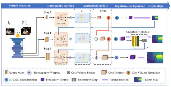
Figure 1. The network architecture of our proposed model. Initially, the multi-scale 2D features are extracted using the cascaded U-Net module. Subsequently, various operations, including homography warping, cost volume aggregation, 3D regularization, and multi-depth classification, are employed to obtain depth estimations at different scales. In Stage 1, the uncertainty module dynamically adjusts the sampling range for the subsequent stage.

3.1. Cascaded U-Net Network

Traditional methods, such as Yao et al. [5], employ 2D convolutional networks for feature extraction, however, this approach can only perceiv image textures within a fixed field of view. In contrast, Chen et al. [33] utilize an improved U-Net network for feature extraction, achieving favorable results. In this section, an enhanced cascaded U-Net feature extraction module is designed. The first part of the structure is illustrated in Figure 2. The network selectively handles low-texture regions to preserve more intricate details.

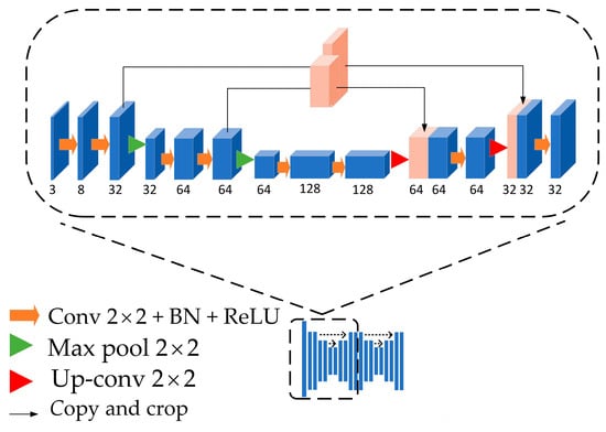
Figure 2. Enhanced cascade U-Net feature extraction module.

The given reference image $I_{i=0}$ and adjacent source images ${\left\{I_i\right\}}_{i=1}^{N-1}$ are fed into the network to construct image features at different scales. In this cascaded U-Net network, the front-end feature encoder utilizes successive convolution and pooling operations, increasing the channel dimensions while reducing the size to extract deep features from the images. However, as the network depth increases, more feature information tends to be lost. The back-end decoder functions inversely to the encoder, performing upsampling to not only restore the original size but also connecting with feature maps from earlier stages. This facilitates better reconstruction of target details. The key to this process lies in fusing high-level and low-level features to enrich the detailed information in the feature maps. Subsequently, the cascaded network repeats this process, and the second part of the cascaded structure appends convolution operations at the output ports, obtaining features $F_{i=0,\dots ,{N-1}_i}^kϵR^{\frac{H}{2^k}\times \frac{W}{2^k}\times 2^{\left(3+k\right)}}$, where $k=0, 1, 2$ denotes the three different stages of the model, omitted for simplicity in the following discussion. This cascaded U-Net feature extraction module aids in preserving richer detailed features, providing more accurate information for depth estimation.

3.2. Homography Warping

In deep learning-based multi-view stereo (MVS) methods [27,29,30], the construction of the cost volume often involves the use of differentiable homographic warping, drawing inspiration from traditional plane sweep stereo. Homographic warping leverage camera parameters to establish mappings between each pixel on the source view and different depths under the reference view, within a depth range of $\left[d_{\mathit{min}},d_{\mathit{max}}\right]$. The procedure entails warping source image features to the $d_j$ layer of the reference view’s viewing frustum. This process is mathematically expressed as shown in Equation (1).

$$p_{s_i,j}=K_i·\left(R_{0,i}·\left(K_0^{-1}·p_r·d_j\right)+t_{0,i}\right)$$

(1)

The pixel feature in the reference view is denoted as $p_r$. We use ${\left\{K_i\right\}}_{i=0}^{N-1}$ to represent the camera intrinsic parameters and ${\left\{\left[R_{0,i}|t_{0,i}\right]\right\}}_{i=1}^{N-1}$ to represent the motion transformation parameters from the source views to the reference view. By embedding camera parameters into features and performing mapping transformations, we establish the mapping relationship between the pixel feature $p_{s_i,j}$ in the i-th source view corresponding to $p_r$. The features $p_{s_i,j}$ are distributed along the epipolar line in the source view, and the depth features of layer $d_j$ can be represented as ${\tilde{F}}_{src,j}=\left\{{\tilde{F}}_{i,j}|i=1\dots N-1\right\}$. Simultaneously, N − 1 feature volumes ${\left\{V_i\right\}}_{i=1}^{N-1}ϵR^{H\times W\times C\times D}$ are generated, where D is the total number of depth hypotheses. This process accomplishes the conversion of features from two-dimensional to three-dimensional, thereby restoring depth information.

Due to the absence of calibration in the input images, directly performing uniform sampling in depth space may result in spatial sampling points not being evenly distributed along the epipolar lines when projected onto the reference view. This is particularly evident in regions farther from the camera center, where the mapped features may be very close, leading to a loss of depth information, as illustrated in Figure 3. To address this issue, inspired by references [29,34], in the first stage of depth sampling, this paper employs the inverse depth sampling method to initialize depth. The specific operation involves uniformly sampling in inverse depth space, ensuring equidistant sampling in pixel space, as shown in Equation (2).

$$d_j={\left(\left(\frac{1}{d_{min}}-\frac{1}{d_{max}}\right)\frac{j}{D-1}+\frac{1}{d_{max}}\right)}^{-1}$$

(2)

Employing this depth sampling method effectively avoids the loss of depth information, thereby significantly enhancing the reconstruction results.

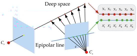
Figure 3. Schematic diagram of depth sampling. When sampling points are evenly spaced in depth space, they may not uniformly map to the epipolar lines corresponding to the source view. This leads to sampling errors and the loss of certain depth information. (In the figure, the depth space and epipolar lines are scaled to the same scale).

3.3. Cost Volume Aggregation

The complete cost volume aggregation module consists of two components: the Epipolar Transformer aggregation module (ET) (Section 3.3.1) and the cross-scale cost volume information exchange module (CVIE) (Section 3.3.2). In this section, we will introduce both components.

3.3.1. Epipolar Transformer

Cost volume construction is the process of aggregating feature volumes from different source views to obtain depth information for individual pixels in the reference view. As conventional variance-based aggregation methods often struggle to filter out noise effectively, this paper employs an epipolar Transformer for aggregating feature volumes from different views. Specifically, the Transformer’s cross-attention mechanism is used to build a 3D correlation along the epipolar line direction between the reference feature $p_r$ (Query) and source features ${\left\{p_{si,j}\right\}}_{j=0}^{D-1}$ (Keys). And use the cross-dimensional attention to guide the aggregation of feature volumes from different views, ultimately achieving cross-dimensional cost volume aggregation. The detailed structure of the module is illustrated in Figure 4.

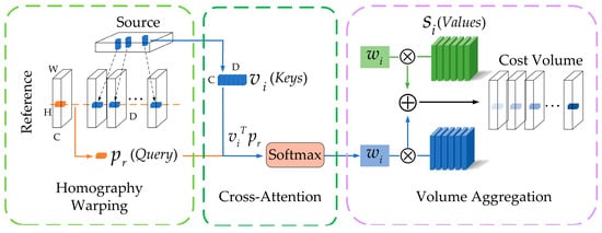
Figure 4. Flowchart of epipolar Transformer aggregation.

Common shallow 2D CNNs can only extract texture features within a fixed receptive field and struggle to capture finer details in regions with weak textures. Therefore, this paper employs the computationally intensive cascaded U-Net for query construction. Guided by Equation (1), the projection transformation of source view features restores the depth information of 2D query features. To ensure 3D consistency in depth space, we adopt a cross-attention mechanism along the epipolar line direction to establish 2D semantic and 3D spatial depth correlations. This involves the 3D correlation between the pixel feature of the reference view, $p_r$ (Query), and the source features mapped to the epipolar line, ${\left\{p_{s_i,j}\right\}}_{j=0}^{D-1}$ (Keys). The attention weights, $w_i$, are computed to achieve this, as shown in Equation (3).

$$w_i=soft\mathit{max}\left(\frac{{v_i}^T{p}_r}{t_e\sqrt{C}}\right),$$

(3)

where $t_e$ represents the temperature parameter. The ${\left\{p_{si,j}\right\}}_{j=0}^{D-1}$ are stacked along the depth dimension to form $v_i\in R^{C\times D}$. Previous studies [35,36] have indicated that utilizing group-wise correlations to group feature volumes can reduce the computational and storage requirements of the model during cost volume construction. Therefore, this paper employs group-wise correlations to partition the feature volumes into $g$ groups along the feature dimension, where $g=0,\dots ,G-1$. Based on the inner product calculation in Equation (4), the similarity $s_i\in R^{G\times D}$ is computed between the source view feature volumes and the reference view feature volume. The obtained $s_i$ serves as the values for the cross-attention mechanism.

$$s_i^g=\frac{1}{G}⟨v_i^g,p_r^g⟩$$

(4)

In this context, the $g$-th group feature of $v_i$ is denoted as $v_i^g\in R^{\frac{C}{G}\times D}$, where $⟨·,·⟩$ represents the inner product. $s_i\in R^{G\times D}$ are obtained by stacking ${\left\{s_i^g\right\}}_{g=0}^{G-1}$ along the channel dimension. Finally, the values of the epipolar attention mechanism are guided and aggregated for stage n by the $w_i$, resulting in the stage-wise aggregated cost volume $C_{agg}^n$. The specific operations are detailed in Formula (5).

$$C_{agg}^n=\frac{{{\displaystyle \sum }}_{i=1}^{N-1}{w}_i{s}_i}{{{\displaystyle \sum }}_{i=1}^{N-1}{w}_i}$$

(5)

3.3.2. Cross-Scale Cost Volume Information Exchange

Traditional multi-view stereo (MVS) algorithms often overlook the correlation between cost volumes at different scales, resulting in a lack of information transfer within each layer [5]. To address this limitation, our study introduces a cross-scale cost volume information exchange module, outlined in Figure 5. To address this, our module employs a portion of the Cascade Iterative Depth Estimation and Refinement (CIDER) [34], applying a lightweight regularization to coarsely regularize the stage-wise cost volume. Subsequently, through a separation operation, this volume is integrated into the next layer. This process eliminates noise and facilitates the fusion of information from small-scale cost volumes into the subsequent layer’s cost volume, thereby enhancing the quality of depth map estimation. It separates the initially regularized stage-wise cost volume, fusing it into the next layer. This process not only eliminates noise but also enables the integration of information from small-scale cost volumes into the next layer, enhancing the quality of depth map estimation. Taking the (n − 1)-th layer as an example, the generated cost $C_{agg}^{n-1}\in R^{B\times C\times D\times H\times W}$ undergoes initial regularization to acquire sufficient contextual information, followed by an upsampling operation, resulting in $C_{agg}^{n-1}\in R^{B\times \raisebox{1ex}{$C$}\!\left/ \!\raisebox{-1ex}{$2$}\right.\times D^{\prime }\times 2H\times 2W}$, where $D$, represents the upsampled depth samples. This size is consistent with the subsequently generated cost volume $C_{agg}^n$ in the next stage. The fusion of these volumes yields the final cost volume $C^n\in R^{B\times C\times D^{\prime }\times 2H\times 2W}$ for that stage.

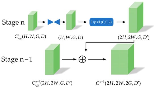
Figure 5. Cross-scale cost volumes information exchange module structure diagram.

3.4. Dynamic Depth Range Sampling

An appropriate depth sampling range is crucial for comprehensive coverage of real depth values, playing a vital role in generating high-quality depth maps. Conventional methods typically focus on the distribution of individual pixels in the probability volume, adjusting the depth sampling range for the next stage based on this information. Zhang et al. [37] introduced a novel approach leveraging the information entropy of a probability volume to fuse feature volumes from different perspectives. Motivated by this, we propose an uncertainty module to adapt the depth sampling range. This module takes the information entropy of the probability volume from Stage 1 as input to assess the reliability of depth inferences. A higher output from the Uncertainty Module indicates greater uncertainty in the current pixel’s depth estimation. Consequently, in Stage 0, the depth sampling range is expanded correspondingly to comprehensively cover true depth values, as illustrated in Figure 1. The module comprises five convolutional layers and activation functions, producing output values between 0 and 1. Higher values signify increased uncertainty. The uncertainty interval $D\left(x\right)$ for the pixel $x$ in the next stage is calculated using Equation (6).

$$D\left(x\right)=\left[D_{est}-\lambda \times U\left(E_{est}\right),D_{est}+\lambda \times U\left(E_{est}\right)\right]$$

(6)

where $\lambda$ is the hyperparameter defining the confidence interval, $E_{est}$ represents the entropy map of the probability volume, $U(·)$ denotes the uncertainty module for the probability volume, and $D_{est}$ is the predicted depth value for the current pixel.

3.5. Multi-Stage Joint Learning

3.5.1. Cross-Entropy Based Learning Objective

Regularization operations yield a probability volume with dimensions $H\times W\times D$, storing the matching probabilities between pixels and different depth values. The paper departs from utilizing the Smooth L₁ loss to minimize the disparity between predicted and actual values. Instead, it addresses a multi-sampled depth value classification problem as an alternative to conventional depth estimation methods. In Stages 0 and 2, the cross-entropy loss function is employed to quantify the difference between the true probability distribution $P\left(x\right)$ and the predicted probability distribution $\widehat{P}\left(x\right)$ for each pixel $x$.

$$L_{class}={\displaystyle \sum }_{x\in \left\{valid\right\}}-\left(P\left(x\right)\log \left(\widehat{P}\left(X\right)\right)+\left(1-P\left(x\right)\right)\log \left(\widehat{P}\left(X\right)\right)\right)$$

(7)

3.5.2. Uncertainty-Based Learning Objectives

In Stage 1, the paper dynamically adjusts the depth sampling range from Stage 0 based on the uncertainty of pixel distribution in the probability volume. Additionally, a negative log-likelihood minimization constraint is incorporated into the loss function of Stage 0 to jointly learn depth value classification and its uncertainty $U(·)$. The loss function for the second stage is outlined in Equation (8).

$$L_{class-uncert}^{stage1}={\displaystyle \sum }_{x\in \left\{valid\right\}}\frac{-\left(P\left(x\right)\log \left(\widehat{P}\left(X\right)\right)+\left(1-P\left(x\right)\right)\log \left(\widehat{P}\left(X\right)\right)\right)}{U\left(x\right)}+\log \left(U\left(x\right)\right)$$

(8)

3.5.3. Joint Learning Objective

The constants ${\lambda }_1,{\lambda }_2$ and ${\lambda }_3$, all belonging to the interval $\left(0,1\right)$, represent the weights assigned to the learning objectives of the three stages. The overarching goal of multi-stage joint learning is to minimize the overall loss function, defined as follows:

$$L_{sum}={\lambda }_1{L}_{class}^{stage0}+{\lambda }_2{L}_{class-uncert}^{stage1}+{\lambda }_3{L}_{class}^{stage2}$$

(9)

4. Experiments

In this section, we evaluate our proposed model on the DTU [38] and Tanks&Temples [39] datasets. We begin by providing a comprehensive overview of the two experimental datasets and detailing the specifics of our experimental setup (Section 4.1 and Section 4.2). Subsequently, we present and analyze the model’s performance on the experimental datasets (Section 4.3). Additionally, we conduct ablation study on the DTU dataset (Section 4.4) to thoroughly validate the effectiveness of our proposed model.

4.1. Datasets

• DTU dataset [38]: This dataset leverages an adjustable industrial robot arm to capture 129 scenes in a laboratory setting. Each scene comprises object views from 64 or 49 different angles under seven distinct lighting conditions, with recorded intrinsic and extrinsic camera parameters. The dataset is partitioned into 79 training scenes, 18 validation scenes, and 22 test scenes. It is noteworthy that we adopt the same dataset partitioning method as CasMVSNet [6].
• Tanks&Temples Dataset [39]: The dataset encompasses 14 indoor and outdoor scenes with varying resolutions. Due to the absence of intrinsic camera parameters in this dataset, we employ OpenMVG [40] (open multiple view geometry) to compute and generate sparse point clouds. Evaluation of the reconstructed point clouds is conducted using an F1 score that combines precision and recall for a comprehensive assessment.

4.2. Implementation Details

Following experimental conventions [30,41], this paper trains and evaluates the proposed model on the DTU dataset. To verify the model’s generalization ability, the model trained on DTU is directly tested on the Tanks&Temples dataset without any modifications. The depth sampling numbers ${\left\{D_k\right\}}_{k=0,1,2}$ at different stages are set to 16, 8, and 4, with depth sampling range ($d_{min}$ and $d_{max}$) configured as 425 mm and 935 mm. The temperature parameter ($t_e$) in the polarcross attention mechanism is set to 2. We train this paper’s model for 14 epoches. The Adam optimizer [42] with ${\beta }_1$ = 0.9 and ${\beta }_2$ = 0.999 is employed to optimize the model. The experiment is conducted on one NVIDIA RTX3090 GPU with a batch size of 2. The initial learning rate is set to 0.001 and is reduced by a factor of 2 after 8, 10, and 12 epoches. For DTU dataset training, input image resolution is 1600 × 1200 with N (number of input images) set to 5. On the Tanks&Temples dataset, N is set to 7, and the input image resolution is 1080 × 2048.

4.3. Benchmark Performance

4.3.1. Evaluation on DTU Dataset

In this section, we compare the performance of our model with traditional methods, learning-based methods, and the methods reported in the latest technical literature.

To better analyze the differences between various methods, our approach is compared with Gipuma [4], Effi-MVSnet [43], DA-PatchmatchNe [44], and CasMVSNet [6]. Among these, Gipuma employs a disparitypropagation strategy from traditional 3D reconstruction methods, proposing a diffusion propagation strategy utilizing GPU’s multicore architecture for multi-view 3D reconstruction. Effi-MVSnet utilizes GRU based on 2D convolution to generate cost volumes. DA-PatchmatchNe combines data augmentation with traditional multi-scale patchmatchalgorithm. Cas-MVSNet adopts a cascaded approach to construct cost volumes, gradually refining the depth sampling range from coarse to fine, ensuring overall efficiency of reconstruction and rational allocation of computational resources.

We opt for input image resolutions of 1600 × 1200 with the number of views set at N = 5. Employing the official evaluation metrics provided by the DTU dataset, we compute reconstruction accuracy (Acc.), completeness (Comp.), and their average, termed overall error (Overall), measuring the reconstruction errors between the generated point cloud and the ground truth. Smaller values of these three metrics indicate better reconstruction performance.

As shown in Table 1, Gipuma [4] achieves the highest score of 0.283 in the Acc. metric, indicating superior performance. While DA-PatchmatchNetbi [44] excels in the Comp. metric with a score of 0.272, our proposed method also achieves impressive results, scoring 0.279, with only a marginal difference of 0.007. Notably, our Overall metric stands at 0.315, leading among all methods. In comparison to the mainstream CasMVSNet [6], we achieve a relative improvement of 11.27%.

Table 1. Experimental results of different methods on the DTU evaluation set (lower values are better). The best and second-best results are highlighted in bold and underlined, respectively.

Method	Acc. (mm)	Comp. (mm)	Overall (mm)
Gipuma [4]	0.283	0.873	0.578
Tola [3]	0.342	1.190	0.766
COLMAP [45]	0.400	0.664	0.532
MVSNet [5]	0.396	0.527	0.462
CIDER [34]	0.417	0.437	0.355
CVP-MVSNet [46]	0.296	0.406	0.351
R-MVSNet [25]	0.383	0.452	0.417
Fast-MVSNet [27]	0.336	0.403	0.370
CasMVSNet [6]	0.325	0.385	0.355
Point-MVSNet [33]	0.342	0.411	0.376
Epp-mvsnet [23]	0.413	0.296	0.355
AA-RMVSNet [8]	0.376	0.339	0.357
UCS-Net [28]	0.338	0.349	0.344
Effi-MVSnet [43]	0.321	0.313	0.317
DA-PatchmatchNet [44]	0.417	0.272	0.344
Ours	0.351	0.279	0.315

Furthermore, Figure 6 illustrates a comparison of the reconstruction results between our method and CasMVSNet [6] in different scenes. The results indicate that the reconstruction outcomes of this paper are denser and exhibit finer details, successfully alleviating the impact of noise in local areas. It is noteworthy that in regions with weak textures, our method preserves more details. This is primarily attributed to the uncertainty dynamic range sampling module, which comprehensively covers real-depth values. Additionally, the introduced cross-scale cost volume information exchange module better handles information connections between different dimensions and scales, further enhancing information utilization. In summary, our proposed algorithm outperforms other methods, showcasing superior competitiveness in terms of reconstruction quality.

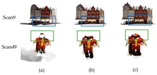
Figure 6. DTU reconstruction results’ comparison. (a) Ground Truth. (b) CasMVSNet reconstruction results. (c) The reconstruction result of our algorithm.

4.3.2. Evaluation on Tanks and Temples Dataset

To assess the generative capability of our approach across diverse scenarios, the model trained on DTU is tested directly on the Tanks&Temples dataset without any adjustments, and compared with traditional methods as well as learning-based methods. During testing, the number of input views is set at N = 7, and the input image size is 1080 × 2048. Evaluation of the reconstructed point cloud is performed using F1 scores, where higher F-scores indicate superior performance.

Table 2 presents the performance comparison with different methods. Our approach maintains outstanding results, scoring an impressive average of 58.60 on the challenging Tanks&Temples intermediate dataset, even with a lower depth sampling rate. This places our method at the forefront, with a marginal 2.91-point gap from the third-ranked AA-RMVSNe [8]. Notably, compared to mainstream methods such as CasMVSNet [6] and Fast-MVSNet [27], our approach showcases performance improvements of 3.86% and 23.65%, respectively. These results affirm the robust generalization capabilities of our model.

Table 2. Quantitative results on the Tanks&Temples dataset—intermediate dataset (F-score, higher is better). F-score is the average across all scenes, and the best and second-best results are highlighted in bold and underlined, respectively.

Method	F-Score	Family	Francis	Horse	Lighthouse	M60	Panther	Playground	Train
ACMH [17]	54.82	69.99	49.45	45.12	59.04	52.64	52.37	58.34	51.61
COLMAP [45]	42.14	50.41	22.25	25.63	56.43	44.83	46.97	48.53	42.04
ACMP [1]	58.41	70.30	54.06	54.11	61.65	54.16	57.60	58.12	57.25
MVSNet [5]	43.48	53.96	34.69	25.07	50.09	55.90	50.86	47.90	28.55
CasMVSNet [6]	56.42	76.36	58.45	46.20	55.33	53.96	54.02	58.17	46.56
DDR-Net [47]	54.91	76.18	53.36	43.43	55.20	55.57	52.28	56.04	47.17
UCS-Net [28]	54.83	76.09	53.16	43.03	54.00	55.60	51.49	57.38	47.89
AA-RMVSNet [8]	61.51	77.77	54.90	51.53	64.02	64.05	59.47	60.85	46.65
Fast-MVSNet [27]	47.39	65.18	39.59	34.98	47.81	49.16	46.20	53.27	42.91
UniMVSN [41]	64.36	81.20	66.43	53.11	63.46	66.09	64.84	62.23	57.53
CVP-MVSNet [46]	54.03	76.50	47.74	36.34	55.12	57.28	54.28	57.43	47.54
PatchmatchNet [29]	53.15	66.99	52.64	43.24	54.87	52.87	49.54	54.21	50.81
Effi-MVS [43]	56.88	72.21	51.02	51.78	58.63	58.71	56.21	57.07	49.38
DA-PatchmatchNet [44]	54.79	68.10	54.60	45.65	57.32	53.43	48.21	57.64	53.33
ET-MVSNet [48]	65.49	81.65	68.79	59.46	65.72	64.22	64.03	61.23	58.79
Ours	58.60	78.23	57.19	48.36	58.25	59.58	56.60	60.36	50.26

4.3.3. Computational Resource Consumption Analysis

To comprehensively evaluate the performance of the proposed model, this experiment presents insights into memory consumption and runtime, comparing them with methods such as AA-RMVSNet [8], CasMVSNet [6], and CIDER [34], as depicted in Figure 7.

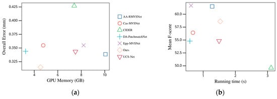
Figure 7. Comparesthe GPU memory usage and runtime of different methods. (a) Contrasts in GPU memory usage. (b) Comparisons of runtime.

Different methods exhibit varying memory usage on the DTU test set, as illustrated in Figure 7a. Through comparison, it is found that our method consumes only 4.53 GB of GPU memory, significantly less than other methods. Meanwhile, among all compared methods, our approach achieves an overall error reduction to 0.315, demonstrating excellent performance. Figure 7b shows the time required for depth map prediction across different methods on the “Tanks&Temples” dataset. Our method computes in just 1.53 s, significantly faster than CIDER. Additionally, our method achieves an F-score of 58.60, demonstrating excellent overall performance.

4.4. Ablation Study

In this section, a series of ablation studies are conducted on the DTU dataset to validate the effectiveness of each component. The official point cloud reconstruction metrics provided by the DTU dataset are employed as experimental benchmarks [38], with default input image specifications set at 864 × 1152. Control variable methodology is employed to isolate the impact of individual components on the overall network performance, ensuring that other components are evaluated under the same experimental conditions.

4.4.1. Number of Views

This experiment, conducted on the DTU dataset, aims to evaluate the impact of different input view counts (N = 3, 4, 5, 6) on reconstruction outcomes. As observed from the results in Table 3, an increase in the number of views allows for the extraction of more feature information, thereby enhancing reconstruction accuracy and completeness. However, indiscriminate addition of views is not a prudent choice, as it not only consumes computational resources but may also introduce unnecessary interference with the overall reconstruction quality. Determining the optimal view count requires a careful balance between performance improvement and efficiency maintenance.

Table 3. Effect of different view numbers on the experimental results.

N	Acc. (mm)	Comp. (mm)	Overall (mm)
3	0.365	0.313	0.339
4	0.360	0.281	0.321
5	0.351	0.279	0.315
6	0.359	0.286	0.323

4.4.2. Cascaded U-Net Network (CU-Net)

The enhanced cascaded U-Net feature extraction module (CU-Net) excels in extracting more precise and comprehensive multi-scale 2D features. It not only emphasizes overall features but also focuses on effectively capturing local details, particularly in handling low-texture areas. This addition enhances sensitivity to local details, leading to superior feature information acquisition. As demonstrated in the experiments in Table 4, this module significantly improves the model’s performance.

Table 4. Effect of CU-Net module on experimental results.

Algorithm	Acc. (mm)	Comp. (mm)	Overall (mm)
None	0.405	0.326	0.366
CU-Net	0.351	0.279	0.315

4.4.3. Dynamic Depth Range Sampling (DDRS)

Table 5 shows the comparative results of the ablation experiment for the dynamic sampling module on the DTU dataset. It can be observed that the dynamic depth range sampling module extends the depth sampling from 13.12 mm to 28.43 mm in stage 0. The coverage of real depth values is also improved, increasing from 0.8468% to 0.8934%. Additionally, even at lower sampling rates, the model’s comprehensive reconstruction error decreases from 0.320 to 0.315. This indicates that measuring the uncertainty of sampling with the entropy of the cost volume, and subsequently adjusting the depth sampling range, allows for more accurate predictions along the object edges. This approach takes into consideration the correlation between contextual information, features of neighboring pixels, and the depth sampling range of the current pixel, resulting in enhanced precision.

Table 5. Quantitative comparison of ablation experiments on dynamic sampling module in DTU’s test set (This experiment mainly analyzes stage 0).

Algorithm	Hypo. Num	Sampling Range (mm)	Coverage Ratio (%)	Overall (mm)
CasMVSNet	48, 32, 8	21.09	0.8441	0.355
DDRNet	48, 32, 8	19.24	0.8435	0.329
Ours	16, 8, 4	13.12	0.8468	0.320
Ours and DDRS	16, 8, 4	28.43	0.8934	0.315

4.4.4. Cost Volume Aggregation

In this experiment, we compare the cost volume construction method proposed in this paper with two types of aggregation in learning-based multi-view stereo (MVS): 1. variance fusing [6,7,28], 2. CNN-based fusing [8,29].

Our method primarily establishes semantic correlations in 3D space through cross-attention, enhancing the aggregation of image features from a greater number of input views during the cost volume construction. Additionally, the cross-scale cost volume communication module boosts information utilization, strengthening correlations among cost volumes at different scales. As demonstrated in Table 6, our approach achieves a relative improvement of 12.35%, 16.01%, and 16.19% in accuracy error, completeness error, and overall error, respectively, compared to CNN aggregation. The reconstruction performance of our method significantly surpasses the other two approaches.

Table 6. Quantitative results of different aggregation methods.

Method	Acc. (mm)	Comp. (mm)	Overall (mm)
CNN Fusion	0.376	0.326	0.351
Variance Fusion	0.353	0.317	0.335
Ours	0.351	0.279	0.315

As depicted in Figure 8, compared to the original CasMVSNet [6] (the number of depth samples is 48, 32, 8), the introduced cost volume aggregation module in our approach helps mitigate the impact of errors, resulting in sharper and smoother edges in the depth map. In Figure 8e, it is evident that our model’s predicted depth map is more complete, demonstrating superior performance in handling low-texture regions and physical edges.

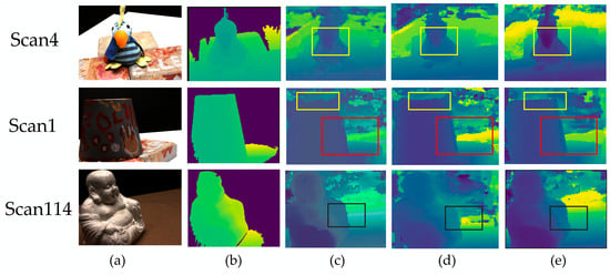
Figure 8. Qualitative comparison of depth map predictions by different methods. (a) Real image. (b) Real depth map. (c) CasMVSNet predicted depth map. (d) CasMVSNet + ET. (e) Depth map predicted by our algorithm.

In Table 7, we conduct ablation study on two components employed in the cost volume aggregation process. Both components show optimization effects on the Overall metric, as evident from the results. It’snoteworthy that the introduction of the CVIE module leads to higher memory usage, primarily due to the additional space required to store the cross-scale cost volume. This addition also increases computation time. However, given the overall performance improvement, the extra storage space is deemed worthwhile.

Table 7. DTU dataset ablation study results’ comparison. Ablation study on the components used in the cost volume aggregation process on the DTU dataset.

Settings		Overall (mm)	Runtime (s)	Param (G)
ET	CVIE
√		0.331	0.21	1.12
	√	0.324	1.53	3.76
√	√	0.315	1.17	4.53

4.4.5. L₁ Loss and Cross-Entropy Loss

In this section, we experimentally compare our classification-based cross-entropy loss (CE loss) with the commonly used regression-based L₁ loss [5,6] on the DTU dataset. The experimental results are presented in Table 8, where the depth error is calculated as the average absolute difference between the predicted depth and the ground truth. Lower error values indicate better performance. It can be observed that replacing the depth regression approach with the multi-depth classification method reduces the depth error from 8.53 to 6.79, and consequently, the overall reconstruction error is further reduced. This validates the effectiveness of the proposed module.

Table 8. Ablation study of L₁ loss and cross-entropy loss on the DTU dataset.

Method	Acc. (mm)	Comp. (mm)	Overall (mm)	Depth Error
$L_1$ loss	0.373	0.281	0.327	8.53
CE loss	0.351	0.279	0.315	6.79

In summary, the excellent reconstruction performance of our method is primarily attributed to the appropriate number of input views, the cascaded U-Net module, the epipolar transformer module, the dynamic depth sampling module, and the multi-stage joint learning approach.

5. Conclusions

This paper proposes an uncertainty-epipolar Transformer multi-view stereo network (U-ETMVSNet) for object stereo reconstruction. Initially, an enhanced Cascaded U-Net is employed to bolster both feature extraction and query construction within the epipolar Transformer. The epipolar Transformer, along with the cross-scale information exchange module, enhances the correlation of cross-dimensional information during cost volume aggregation, ensuring 3D consistency in depth space. The dynamic adjustment of depth sampling range based on the uncertainty of the probability volume also enhance stability in reconstructing regions with weak texture, and the reconstruction performance remains excellent even at lower depth sampling rates. Finally, the multi-stage joint learning method based on multi-depth value classification solution also effectively improves the reconstruction accuracy. The proposed method in this paper exhibits excellent performance in terms of completeness, accuracy, and generalization ability on the DTU and Tanks&Temples datasets, comparable to existing mainstream CNN-based MVS networks. However, the algorithm retains common 3D CNN regularization modules, resulting in no significant advantage in terms of memory usage. Future work aims to explore the role of Transformers in dense feature matching to replace CNN regularization, enhancing the practicality of deploying the model on mobile devices.

References

- Campbell, N.D.; Vogiatzis, G.; Hernández, C.; Cipolla, R. Using multiple hypotheses to improve depth-maps for multi-view stereo. In Proceedings of the Computer Vision–ECCV 2008: 10th European Conference on Computer Vision, Marseille, France, 12–18 October 2008; Proceedings, Part I 10. pp. 766–779. [Google Scholar]
- Galliani, S.; Lasinger, K.; Schindler, K. Gipuma: Massively parallel multi-view stereo reconstruction. Publ. Dtsch. Ges. Photogramm. Fernerkund. Geoinf. E. V 2016, 25, 2. [Google Scholar]
- Tola, E.; Strecha, C.; Fua, P. Efficient large-scale multi-view stereo for ultra high-resolution image sets. Mach. Vis. Appl. 2012, 23, 903–920. [Google Scholar] [CrossRef]
- Galliani, S.; Lasinger, K.; Schindler, K. Massively parallel multiview stereopsis by surface normal diffusion. In Proceedings of the IEEE International Conference on Computer Vision, Santiago, Chile, 7–13 December 2015; pp. 873–881. [Google Scholar]
- Yao, Y.; Luo, Z.; Li, S.; Fang, T.; Quan, L. Mvsnet: Depth inference for unstructured multi-view stereo. In Proceedings of the European Conference on Computer Vision (ECCV), Munich, Germany, 8–14 September 2018; pp. 767–783. [Google Scholar]
- Gu, X.; Fan, Z.; Zhu, S.; Dai, Z.; Tan, F.; Tan, P. Cascade cost volume for high-resolution multi-view stereo and stereo matching. In Proceedings of the IEEE/CVF Conference on Computer Vision and Pattern Recognition, Seattle, WA, USA, 13–19 June 2020; pp. 2495–2504. [Google Scholar]
- Xu, H.; Zhang, J. Aanet: Adaptive aggregation network for efficient stereo matching. In Proceedings of the IEEE/CVF Conference on Computer Vision and Pattern Recognition, Seattle, WA, USA, 13–19 June 2020; pp. 1959–1968. [Google Scholar]
- Wei, Z.; Zhu, Q.; Min, C.; Chen, Y.; Wang, G. Aa-rmvsnet: Adaptive aggregation recurrent multi-view stereo network. In Proceedings of the IEEE/CVF International Conference on Computer Vision, Montreal, BC, Canada, 11–17 October 2021; pp. 6187–6196. [Google Scholar]
- Yi, H.; Wei, Z.; Ding, M.; Zhang, R.; Chen, Y.; Wang, G.; Tai, Y.-W. Pyramid multi-view stereo net with self-adaptive view aggregation. In Proceedings of the Computer Vision–ECCV 2020: 16th European Conference, Glasgow, UK, 23–28 August 2020; Proceedings, Part IX 16. pp. 766–782. [Google Scholar]
- Luo, K.; Guan, T.; Ju, L.; Huang, H.; Luo, Y. P-mvsnet: Learning patch-wise matching confidence aggregation for multi-view stereo. In Proceedings of the IEEE/CVF International Conference on Computer Vision, Seoul, Republic of Korea, 27 October–2 November 2019; pp. 10452–10461. [Google Scholar]
- Yu, A.; Guo, W.; Liu, B.; Chen, X.; Wang, X.; Cao, X.; Jiang, B. Attention aware cost volume pyramid based multi-view stereo network for 3d reconstruction. ISPRS J. Photogramm. Remote Sens. 2021, 175, 448–460. [Google Scholar] [CrossRef]
- Li, Z.; Liu, X.; Drenkow, N.; Ding, A.; Creighton, F.X.; Taylor, R.H.; Unberath, M. Revisiting stereo depth estimation from a sequence-to-sequence perspective with transformers. In Proceedings of the IEEE/CVF International Conference on Computer Vision, Montreal, BC, Canada, 11–17 October 2021; pp. 6197–6206. [Google Scholar]
- Stereopsis, R.M. Accurate, Dense, and Robust Multiview Stereopsis. IEEE Trans. Pattern Anal. Mach. Intell. 2010, 32, 1362–1376. [Google Scholar]
- Lhuillier, M.; Quan, L. A quasi-dense approach to surface reconstruction from uncalibrated images. IEEE Trans. Pattern Anal. Mach. Intell. 2005, 27, 418–433. [Google Scholar] [CrossRef] [PubMed]
- Sinha, S.N.; Mordohai, P.; Pollefeys, M. Multi-view stereo via graph cuts on the dual of an adaptive tetrahedral mesh. In Proceedings of the IEEE 11th International Conference on Computer Vision, Rio De Janeiro, Brazil, 14–21 October 2007; pp. 1–8. [Google Scholar]
- Zheng, E.; Dunn, E.; Jojic, V.; Frahm, J.-M. Patchmatch based joint view selection and depthmap estimation. In Proceedings of the IEEE Conference on Computer Vision and Pattern Recognition, Columbus, OH, USA, 23–28 June 2014; pp. 1510–1517. [Google Scholar]
- Xu, Q.; Tao, W. Multi-scale geometric consistency guided multi-view stereo. In Proceedings of the IEEE/CVF Conference on Computer Vision and Pattern Recognition, Long Beach, CA, USA, 15–20 June 2019; pp. 5483–5492. [Google Scholar]
- Fei, L.; Yan, L.; Chen, C.; Ye, Z.; Zhou, J. Ossim: An object-based multiview stereo algorithm using ssim index matching cost. IEEE Trans. Geosci. Remote Sens. 2017, 55, 6937–6949. [Google Scholar] [CrossRef]
- Li, Z.; Wang, K.; Zuo, W.; Meng, D.; Zhang, L. Detail-preserving and content-aware variational multi-view stereo reconstruction. IEEE Trans. Image Process. 2015, 25, 864–877. [Google Scholar] [CrossRef] [PubMed]
- Vogiatzis, G.; Esteban, C.H.; Torr, P.H.; Cipolla, R. Multiview stereo via volumetric graph-cuts and occlusion robust photo-consistency. IEEE Trans. Pattern Anal. Mach. Intell. 2007, 29, 2241–2246. [Google Scholar] [CrossRef] [PubMed]
- Ji, M.; Gall, J.; Zheng, H.; Liu, Y.; Fang, L. Surfacenet: An end-to-end 3d neural network for multiview stereopsis. In Proceedings of the IEEE International Conference on Computer Vision, Venice, Italy, 22–29 October 2017; pp. 2307–2315. [Google Scholar]
- Huang, P.-H.; Matzen, K.; Kopf, J.; Ahuja, N.; Huang, J.-B. Deepmvs: Learning multi-view stereopsis. In Proceedings of the IEEE Conference on Computer Vision and Pattern Recognition, Salt Lake City, UT, USA, 18–23 June 2018; pp. 2821–2830. [Google Scholar]
- Ma, X.; Gong, Y.; Wang, Q.; Huang, J.; Chen, L.; Yu, F. Epp-mvsnet: Epipolar-assembling based depth prediction for multi-view stereo. In Proceedings of the IEEE/CVF International Conference on Computer Vision, Montreal, BC, Canada, 11–17 October 2021; pp. 5732–5740. [Google Scholar]
- Yang, J.; Mao, W.; Alvarez, J.M.; Liu, M. Cost volume pyramid based depth inference for multi-view stereo. In Proceedings of the IEEE/CVF Conference on Computer Vision and Pattern Recognition, Seattle, WA, USA, 13–19 June 2020; pp. 4877–4886. [Google Scholar]
- Yao, Y.; Luo, Z.; Li, S.; Shen, T.; Fang, T.; Quan, L. Recurrent mvsnet for high-resolution multi-view stereo depth inference. In Proceedings of the IEEE/CVF Conference on Computer Vision and Pattern Recognition, Long Beach, CA, USA, 15–20 June 2019; pp. 5525–5534. [Google Scholar]
- Chen, R.; Han, S.; Xu, J.; Su, H. Visibility-aware point-based multi-view stereo network. IEEE Trans. Pattern Anal. Mach. Intell. 2020, 43, 3695–3708. [Google Scholar] [CrossRef] [PubMed]
- Yu, Z.; Gao, S. Fast-mvsnet: Sparse-to-dense multi-view stereo with learned propagation and gauss-newton refinement. In Proceedings of the IEEE/CVF Conference on Computer Vision and Pattern Recognition, Seattle, WA, USA, 13–19 June 2020; pp. 1949–1958. [Google Scholar]
- Cheng, S.; Xu, Z.; Zhu, S.; Li, Z.; Li, L.E.; Ramamoorthi, R.; Su, H. Deep stereo using adaptive thin volume representation with uncertainty awareness. In Proceedings of the IEEE/CVF Conference on Computer Vision and Pattern Recognition, Seattle, WA, USA, 13–19 June 2020; pp. 2524–2534. [Google Scholar]
- Wang, F.; Galliani, S.; Vogel, C.; Speciale, P.; Pollefeys, M. Patchmatchnet: Learned multi-view patchmatch stereo. In Proceedings of the IEEE/CVF Conference on Computer Vision and Pattern Recognition, Nashville, TN, USA, 20–25 June 2021; pp. 14194–14203. [Google Scholar]
- Ding, Y.; Yuan, W.; Zhu, Q.; Zhang, H.; Liu, X.; Wang, Y.; Liu, X. Transmvsnet: Global context-aware multi-view stereo network with transformers. In Proceedings of the IEEE/CVF Conference on Computer Vision and Pattern Recognition, New Orleans, LA, USA, 18–24 June 2022; pp. 8585–8594. [Google Scholar]
- Zhu, J.; Peng, B.; Li, W.; Shen, H.; Zhang, Z.; Lei, J. Multi-view stereo with transformer. arXiv 2021, arXiv:2112.00336. [Google Scholar]
- Sun, J.; Shen, Z.; Wang, Y.; Bao, H.; Zhou, X. LoFTR: Detector-free local feature matching with transformers. In Proceedings of the IEEE/CVF Conference on Computer Vision and Pattern Recognition, Nashville, TN, USA, 20–25 June 2021; pp. 8922–8931. [Google Scholar]
- Chen, R.; Han, S.; Xu, J.; Su, H. Point-based multi-view stereo network. In Proceedings of the IEEE/CVF International Conference on Computer Vision, Seoul, Republic of Korea, 27 October–2 November 2019; pp. 1538–1547. [Google Scholar]
- Xu, Q.; Tao, W. Learning inverse depth regression for multi-view stereo with correlation cost volume. In Proceedings of the AAAI Conference on Artificial Intelligence, New York, NY, USA, 7–12 February 2020; pp. 12508–12515. [Google Scholar]
- Chong, A.; Yin, H.; Liu, Y.; Wan, J.; Liu, Z.; Han, M. Multi-hierarchy feature extraction and multi-step cost aggregation for stereo matching. Neurocomputing 2022, 492, 601–611. [Google Scholar] [CrossRef]
- Zhang, J.; Yao, Y.; Li, S.; Luo, Z.; Fang, T. Visibility-aware multi-view stereo network. arXiv 2020, arXiv:2008.07928. [Google Scholar]
- Zhang, J.; Li, S.; Luo, Z.; Fang, T.; Yao, Y. Vis-mvsnet: Visibility-aware multi-view stereo network. Int. J. Comput. Vis. 2023, 131, 199–214. [Google Scholar] [CrossRef]
- Aanæs, H.; Jensen, R.R.; Vogiatzis, G.; Tola, E.; Dahl, A.B. Large-scale data for multiple-view stereopsis. Int. J. Comput. Vis. 2016, 120, 153–168. [Google Scholar] [CrossRef]
- Knapitsch, A.; Park, J.; Zhou, Q.-Y.; Koltun, V. Tanks and temples: Benchmarking large-scale scene reconstruction. ACM Trans. Graph. (ToG) 2017, 36, 1–13. [Google Scholar] [CrossRef]
- Tsoi, K.W. Improve OpenMVG and Create a Novel Algorithm for Novel View Synthesis from Point Clouds; University of Illinois at Urbana-Champaign: Champaign, IL, USA, 2016. [Google Scholar]
- Peng, R.; Wang, R.; Wang, Z.; Lai, Y.; Wang, R. Rethinking depth estimation for multi-view stereo: A unified representation. In Proceedings of the IEEE/CVF Conference on Computer Vision and Pattern Recognition, New Orleans, LA, USA, 18–24 June 2022; pp. 8645–8654. [Google Scholar]
- Kinga, D.; Adam, J.B. A method for stochastic optimization. In Proceedings of the International Conference on Learning Representations (ICLR), San Diego, CA, USA, 7–9 May 2015; p. 6. [Google Scholar]
- Wang, S.; Li, B.; Dai, Y. Efficient multi-view stereo by iterative dynamic cost volume. In Proceedings of the IEEE/CVF Conference on Computer Vision and Pattern Recognition, New Orleans, LA, USA, 18–24 June 2022; pp. 8655–8664. [Google Scholar]
- Pan, F.; Wang, P.; Wang, L.; Li, L. Multi-View Stereo Vision Patchmatch Algorithm Based on Data Augmentation. Sensors 2023, 23, 2729. [Google Scholar] [CrossRef] [PubMed]
- Schonberger, J.L.; Frahm, J.-M. Structure-from-motion revisited. In Proceedings of the IEEE Conference on Computer Vision and Pattern Recognition, Las Vegas, NV, USA, 27–30 June 2016; pp. 4104–4113. [Google Scholar]
- Gao, S.; Li, Z.; Wang, Z. Cost volume pyramid network with multi-strategies range searching for multi-view stereo. In Proceedings of the Computer Graphics International Conference, Online, 12–16 September 2022; pp. 157–169. [Google Scholar]
- Yi, P.; Tang, S.; Yao, J. DDR-Net: Learning multi-stage multi-view stereo with dynamic depth range. arXiv 2021, arXiv:2103.14275. [Google Scholar]
- Liu, T.; Ye, X.; Zhao, W.; Pan, Z.; Shi, M.; Cao, Z. When Epipolar Constraint Meets Non-local Operators in Multi-View Stereo. In Proceedings of the IEEE/CVF International Conference on Computer Vision, Paris, France, 2–6 October 2023; pp. 18088–18097. [Google Scholar]
Disclaimer/Publisher’s Note: The statements, opinions and data contained in all publications are solely those of the individual author(s) and contributor(s) and not of MDPI and/or the editor(s). MDPI and/or the editor(s) disclaim responsibility for any injury to people or property resulting from any ideas, methods, instructions or products referred to in the content. |
© 2024 by the authors. Licensee MDPI, Basel, Switzerland. This article is an open access article distributed under the terms and conditions of the Creative Commons Attribution (CC BY) license (https://creativecommons.org/licenses/by/4.0/).