Method for Sparse Representation of Complex Data Based on Overcomplete Basis, l₁ Norm, and Neural MFNN-like Network

Abstract

The article presents the results of research into a method for representing complex data based on an overcomplete basis and l₀/l₁ norms. The proposed method is an extended modification of the neural-like MFNN (minimum fuel neural network) for the case of complex data. The influence of the choice of activation function on the performance of the method is analyzed. The results of the numerical simulation demonstrate the effectiveness of the proposed method for the case of sparse representation of complex data and can be used to determine the direction of arrival (DOA) for a uniform linear array (ULA).

1. Introduction

Classical methods for presenting data based on a selected basis include fast Fourier transform algorithms, cosine transform, wavelet transform, etc. The concept of an overcomplete basis is the use of a basis with a significantly larger number of components compared to the number of components in the analyzed data, which leads to the so-called SR (sparse representation). Unlike classical methods, the elements of the basis may not necessarily be functions orthogonal to each other, but the method of data representation is based on their decomposition into a number of optimal basic components, which are found from an overly complete basis dictionary using optimization algorithms such as, for example, MP (matching pursuit) and MOF (method of frame), using different norms [1,2,3,4,5,6,7,8,9,10]. The overcomplete basis or basis components are specified a priori or found using some optimization algorithms, such as correspondence search, frame methods, and basis search, depending on the current characteristics of the received data.

One of the important classes of norms [11] is the so-called l_p norms for vector x. representing dimension I:

$$l_p={\left({\displaystyle \sum }_{i=1}^I{\left|x_i\right|}^p\right)}^{1/p} \mathrm{for} p\ge 1$$

(1)

For the occasion p = 0:

$$l_0=\left({\displaystyle \sum }_{i=1}^I{\left|x_i\right|}^0\right), {\left|x_i\right|}^0=\left\{\begin{array}{ll}0,\hspace{1em}& \mathit{if} x_i=0\\ 1,\hspace{1em}& \mathrm{otherwise}\end{array}\right.$$

(2)

Thus, l₀ is the number of non-zero elements in x. Minimizing the l₀ norm leads to maximizing the number of zero values and to sparse data [12].

For the occasion p = 1:

$$l_1=\left({\displaystyle \sum }_{i=1}^I{\left|x_i\right|}^1\right)$$

(3)

Norm l₁ represents the sum of the absolute values of elements in x and is widely used in algorithms such as LASSO (least absolute shrinkage and selection operator) in statistics BP (basis pursuit) in signal processing [12].

It should be noted that methods using SR can effectively separate coherent sources because data evaluation is based on an optimization method, such as l₁ norm minimization, rather than on sub-space orthogonality, as in MUSIC (multiple signal classification) [13] or MVDR (minimum variance distortion less response) [14] and their use [15]. In addition, if the noise variance value used as the regularization parameter does not match the environmental noise variance, the evaluation performances of the corresponding methods are significantly degraded. An essential point is that when solving highly sparse linear optimization problems, the l₁ norm is equivalent to the l₀ norm, including for complex data [16,17].

The solutions given in [18,19] also allow the representation of data in an overcomplete dictionary basis. Along with the methods mentioned earlier, the decomposition of data into weighted dictionary components can be presented in the form of the so-called “fuel minimization” problem or MFNN [19], which is an optimization problem in a basis with norm l₁ linear restrictions. Extending it to the complex plane ℂ, we obtain:

$$\begin{gathered} \left\{ma{x}_{y\in \mathsf{\Omega }} y^{T}x\right\}\to min \\ \mathrm{given} \mathrm{that} Ax=b, \end{gathered}$$

(4)

where $\mathsf{\Omega }=\left\{\omega \in {ℂ}^N\left|\left|{\omega }_i\right|\le 1\right.,i-1,2,\dots ,N\right\}\subset {ℂ}^N,b\in {ℂ}^M$ represents the input data,

• $x={\left[{\alpha }_{{\gamma }_1}{\alpha }_{{\gamma }_2}\dots {\alpha }_{{\gamma }_N}\right]}^T\in {ℂ}^N$ represents the basic components,
• $A=\left[{\varphi }_{{\gamma }_1},{\varphi }_{{\gamma }_2},\dots ,{\varphi }_{{\gamma }_N}\right]\in {ℂ}^{M\times N}$ represents the overcomplete dictionary matrix.
• $D=({\varphi }_{\gamma })$formed dictionary, where ${\varphi }_{\gamma }\in {ℂ}^{M }$ is the component of the basis with indexes $\gamma \in \mathsf{\Gamma } \mathrm{and} \mathsf{\Gamma }\subset L^2\left(ℝ\right)$

The input data S can be represented as:

$$b={\sum }_{i=1}^N{\alpha }_{{\gamma }_i}{\varphi }_{{\gamma }_i}+r^{\left(N+1\right)},$$

(5)

where $r^{\left(N+1\right)}\in {ℂ}^M$—the residual vector or error vector—is the result of the approximation of data b by the basis functions ${\varphi }_{{\gamma }_1},{\varphi }_{{\gamma }_2},\dots ,{\varphi }_{{\gamma }_N}$ from the dictionary D, and ${\alpha }_{{\gamma }_i}$- i- is the weight coefficient.

The solution to the optimization problem can be obtained by minimizing the norm of the loss function:

$$J={\Vert r^{\left(N+1\right)}\Vert }_p={\Vert b-Ax\Vert }_p,$$

(6)

where ${\Vert \Vert }_p$ is the p-norm; in general, p = 2 (norm l₂), and p = 1 (norm l₁).

There are two approaches to solving this problem for p = 1. The first approach is described as an MP algorithm. This approach operates with dictionaries obtained from wavelet dictionaries, orthogonal dictionaries, and cosine functions. The second approach is called BP (basis pursuit) and was proposed by Chen and Donoho [16]. It operates with a simple dictionary of basis functions and allows the finding of an estimate of x using the BCSV (Box–Cox stochastic volatility) method by minimizing the l₁ norm of x.

An implementation option for the Algorithm 1 BP—IRLS (iteratively reweighted least squares) [20] is given below:

Algorithm 1: BP

Start:$\mathrm{Basis} \mathrm{matrix} A\in {ℝ}^{m\times N}$$, \mathrm{data} \mathrm{vector} y\in {ℝ}^m$$, \mathrm{initial} \mathrm{value} \mathrm{of} \mathrm{the} \mathrm{scales}$ ${\omega }_0\in {ℝ}^N$$(\mathrm{by} \mathrm{default}: {\omega }_0=\left(1, 1, \dots , 1\right)$). ${\epsilon }_0=\infty$ for$k=0, 1, 2, \dots$do           $x^{k+1}:=\arg \underset{z\in {ℝ}^N}{\min }z, \mathrm{diag} \left({\omega }_k\right)z$$\mathrm{subject} \mathrm{to} Az=y$,           ${\epsilon }_{k+1}:=\min \left({\epsilon }_k, \frac{{\sigma }_s{\left(x^{k+1}\right)}_{l_1}}{N}\right),$           ${\left({\omega }_{k+1}\right)}_i:=\frac{1}{\max \left(\left|x_i^{k+1}\right|,{\epsilon }_{k+1}\right)} \mathrm{for} \mathrm{each} i\in \left[N\right]$ end for return Sequence${\left(x^k\right)}_{k\ge 1}$

where ${\sigma }_s{\left(x\right)}_{l_1}=\inf \left\{x-z_1:z\in {ℝ}^N \mathrm{is} s-\mathrm{sparse}\right\}$.

However, the algorithm is still not fast enough, and it does not allow the use of complex data.

In [21,22,23], Algorithm 2 SL0 (smoothed l₀ norm) is presented, which implements a fairly fast method of finding a sparse solution to an uncertain system of linear equations, including for complex data. The SL0 algorithm implements an approximate solution based on the gradient method, with step-by-step projection of the result onto the space of feasible vectors:

Algorithm 2: SL0

Start: b, A, [σ1, …, σK], μ Initialization:$x_1=x_0$ Cycle in k with a given number of repetitions:   $∆x=x_k\exp \left({\left|x_k\right|}^2/2{\mathsf{\sigma }}_k^2\right)$    $x_k=\left(x_{k-1}-\mu {\displaystyle \blacksquare }∆x\right)-A^H{\left(A{A}^H\right)}^{-1}\left(A{x}_{k-1}-b\right)$

where b is the initial coefficient of the scales, A is the selected excess basis matrix, σ and μ are coefficients determining the speed of convergence, and x is the solution vector.

However, despite the high speed of convergence, this algorithm is sensitive to the choice of initial values of the coefficients and does not guarantee convergence to the optimal solution.

Summarizing the above, we can highlight three characteristic points regarding this algorithm:

(1)

Minimizing the loss function leads to minimizing the number of non-zero components in vector x.

(2)

Based on the perturbation theory, the l₁ norm is more robust compared to the l₂ norm, which affects the quality of processing of non-stationary signals that contain sections of transient processes.

(3)

From a computational point of view, the problem belongs to the LP problem (linear programming, the class of optimization problems).

In [18], approaches to solving systems of linear equations based on neural networks are presented. In [19], a solution to the fuel minimization problem is presented in the form of a neural network MFNN, an example of which, from [19] for M = 8 and N = 3, is shown in Figure 1, which is described by a system of differential equations of the form:

$$\left\{\begin{array}{c}\frac{dx}{dt}=-A^T\left[Ax-y-b\right]-P_{\mathsf{\Omega }}\left(x+A^{T}y\right),\\ \frac{dy}{dt}=-A\left[x+A^{T}y-P_{\mathsf{\Omega }}\left(x+A^{T}y\right)\right]+b,\end{array}\right.$$

(7)

$$z=x+A^{T }y, \mathrm{z} ∊ {ℂ}^N$$

where $P_{\mathsf{\Omega }}\left(z\right)={\left[P_{\mathsf{\Omega }}\left(z_1\right),P_{\mathsf{\Omega }}\left(z_2\right),\dots ,P_{\mathsf{\Omega }}\left(z_n\right)\right]}^T$ is the activation function (8):

$$P_{\mathsf{\Omega }}\left(z_i\right)=\frac{1}{2}\left(\left|z_i+1\right|-\left|z_i-1\right|\right)=\left\{\begin{array}{cc}\hfill 1,& if z_i>1\hfill \\ \hfill -1,& if z_i<-1\hfill \\ \hfill z_i,& \mathrm{otherwise} \hfill \end{array}\right.$$

(8)

Cosine functions are used as a dictionary in [19]. Methods for forming a dictionary, in particular, are described in [16], which also shows the relationship between increasing the redundancy of the dictionary and the quality of data approximation when defining linear programming problems. In [19], it is shown that in the field of real numbers ℝ, the neural network described by the system Equation (7) gives a solution that is globally stable according to Lyapunov and approaches the exact detection of problem (4).

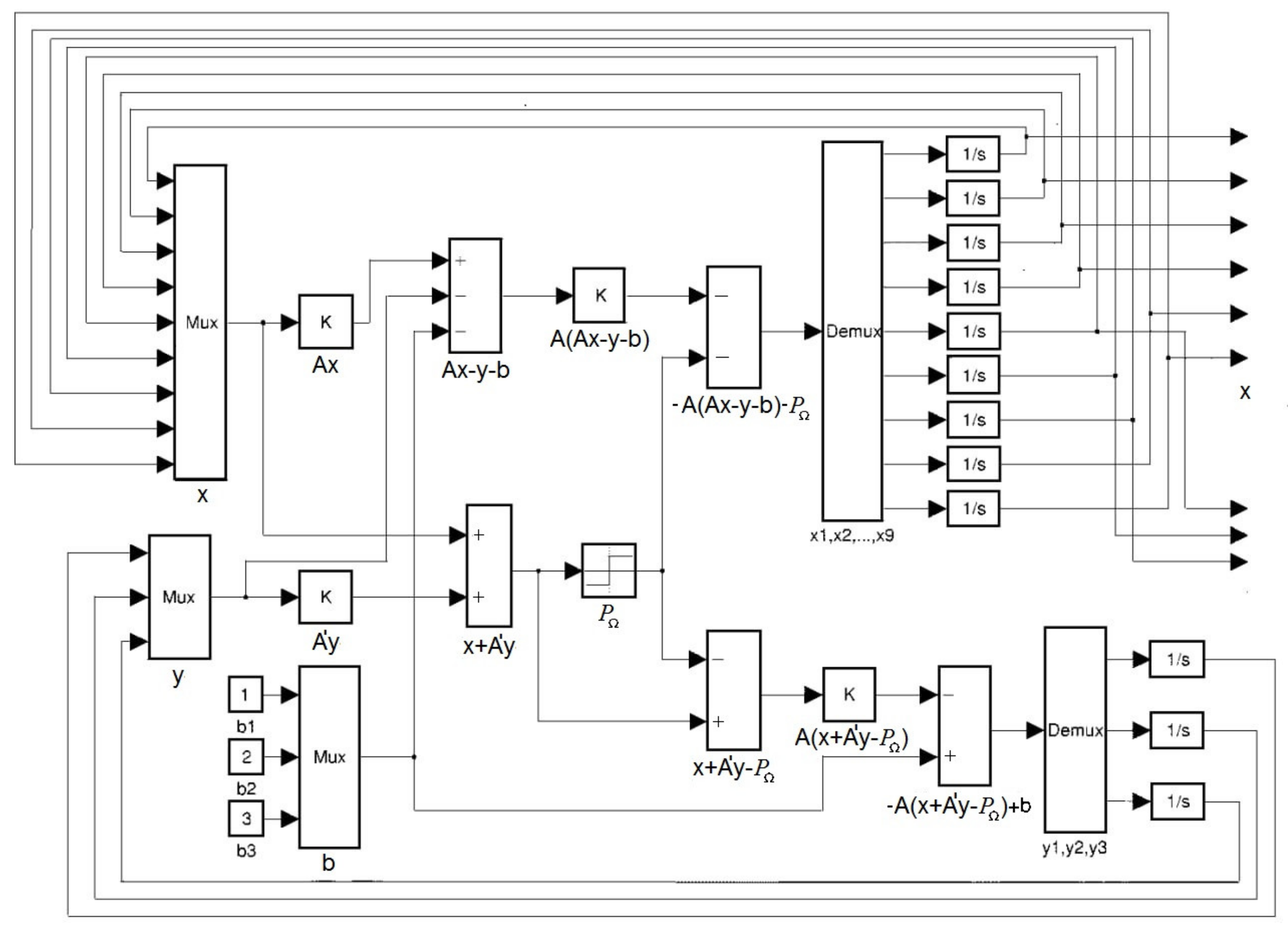
2. Minimum Fuel Neural Network for Complex Data

The described approaches were used in [18,19] for certain classes of real data. To process complex data, it is necessary to refine the presented approaches in terms of forming a dictionary and the logic of the activation function (8).

Let us consider, as an example, an algorithm for forming a dictionary for data representing complex signals, after transferring to zero frequency, received by the ULA:

$$b_{k,m}={\dot{b}}_k{\mathrm{e}}^{j2\mathsf{\pi }d\left(m-1\right)\sin \left({\theta }_k\right)},$$

(9)

where k = 1, 2, …, K, K is the number of point external sources, ${\theta }_k$ is the angular direction to the k-th source,${\dot{b}}_k$ is the amplitude of the k-th source, d is the lattice element pitch normalized to the wavelength, and $j=\sqrt{-1}$.

Then, the elements of the overcomplete basis dictionary matrix can be represented as:

$$A_{m,i}=b_k{\mathrm{e}}^{j2\mathsf{\pi }d\left(m-1\right)\sin \left({\theta }_i\right)},$$

(10)

where ${\theta }_i=\frac{180°·i}{N}-90°$), i = 1, 2, …, N is the dimension of the angular direction grid of the overcomplete basis dictionary, and m = 1, 2, …, M. (M is the number of receiving elements of the antenna array.)

There are two possible implementation options for the minimum fuel neural network MFNN, based on the structure presented in Figure 1.

The first option for implementing the neural system under consideration is the option with the presentation of complex input data b = Re (b) + j Jm(b), specified as a double-length real data vector b = [Re(b₁), …, Re(b_M), Jm(b₁), …, Jm(b_M)]; then, the vector of the resulting basis components (solutions) X = Re(X) + j Jm(X) similarly can be represented in the form:

$$X={\left[\mathrm{Re}\left(x_1\right) \mathrm{Re}\left(x_2\right)\dots \mathrm{Re}\left(x_N\right) \mathrm{Im}\left(x_1\right) \mathrm{Im}\left(x_2\right)\dots \mathrm{Im}(x_N)\right]}^T$$

(11)

The algorithm for forming a dictionary in this case will be as follows:

(1)

A grid of angular directions to the source can be formed with a uniform step both in wave numbers ${\phi }_i=\frac{\pi }{N}\left(i-1\right)-\frac{\pi }{2}$ and in the angle $\sin \left({\phi }_i\right)$, where i = 1, 2, …, N is the total number of angular directions. In the first case, it turns out to be denser in the vicinity of the zero-angle value.

(2)

For an m-channel receiving system, two parts of the dictionary are formed in the following ways:

$$\begin{gathered} A_1=\sin (\pi \left(m-1\right)\sin \left({\phi }_i\right)), \\ {A}_2=\cos (\pi \left(m-1\right)\sin \left({\phi }_i\right)) \end{gathered}$$

(12)

(3)

The formed parts are combined into a common dictionary, according to the rule:

$$A=\left(\begin{array}{c}A1 -A2\\ A2 A1\end{array}\right),$$

(13)

In this case, all operations on data in the neural network will be carried out with real values.

The second option for implementing a neural network is the option of replacing real variables with complex ones and performing all operations with complex values.

The form of the system of Equation (7) in both the first and second cases will remain unchanged. The choice of one of the options will be determined only by the convenience of the specific hardware and software implementations. At the same time, since the absolute values of the real and complex variables are defined differently, the question arises of choosing the optimal form of the activation function P_Ω for the case of using complex data.

3. Activation Function to Implement the Algorithm in Real Form

If we do not make changes to activation function (8), then for the implementation option with the representation of a vector of complex data by a vector of real data, twice the length of (11), we will obtain it in the form of a simple limiter:

$$P_{\mathsf{\Omega }}\left(\dot{z}\right)={\left[P_{\mathsf{\Omega }}\left({\dot{z}}_1\right) P_{\mathsf{\Omega }}\left({\dot{z}}_2\right)\dots P_{\mathsf{\Omega }}\left({\dot{z}}_N\right) P_{\mathsf{\Omega }}\left({\dot{z}}_{N+1}\right) P_{\mathsf{\Omega }}\left({\dot{z}}_{N+2}\right)\dots P_{\mathsf{\Omega }}\left({\dot{z}}_{2N}\right)\right]}^T$$

(14)

where $\left.\begin{array}{c}{\dot{z}}_i=\mathrm{Re}\left(z_i\right)\\ {\dot{z}}_{i+N}=\mathrm{Im}\left(z_i\right)\end{array}\right\},$

$$P_{\mathsf{\Omega }}\left({\dot{z}}_i\right)=\left\{\begin{array}{c}1, \mathrm{if} \left|{\dot{z}}_i\right|>1\\ -1, \mathrm{if} \left|{\dot{z}}_i\right|<-1\\ {\dot{z}}_i, \mathrm{otherwise} \end{array} ,i=1, 2,\dots , 2N \right.$$

(15)

Another option for the activation function is to represent it in the form:

$$P_{\mathsf{\Omega }}\left({\dot{z}}_i\right)=\left\{\begin{array}{cc}\hfill \frac{{\dot{z}}_i}{\left|w_i\right|},& \mathrm{if} \left|{\dot{w}}_i\right|>1\hfill \\ \hfill {\dot{z}}_i,& \mathrm{if} \left|{\dot{w}}_i\right|\le 1\hfill \end{array}\right. , P_{\mathsf{\Omega }}\left({\dot{z}}_{i+N}\right)=\left\{\begin{array}{c}\frac{{\dot{z}}_{i+N}}{\left|{\dot{w}}_i\right|}, \mathrm{if} \left|{\dot{w}}_i\right|>1\\ {\dot{z}}_{i+N}, \mathrm{if} \left|{\dot{w}}_i\right|\le 1\end{array}\right.$$

(16)

where $\left|{\dot{w}}_i\right|=\sqrt{{\dot{z}}_i^2+{\dot{z}}_{i+N}^2}, i=1,2,\dots ,N$, and $\left|{\dot{w}}_{i+N}\right|=\left|{\dot{w}}_i\right|, i=1,2,\dots ,N$.

One more possible option for the activation function is the following:

$$\left[P_{\mathsf{\Omega }}\left({\dot{z}}_i\right),P_{\mathsf{\Omega }}\left({\dot{z}}_{i+N}\right)\right]=\left\{\begin{array}{cc}\hfill \left[\frac{{\dot{z}}_i}{\left|{\dot{z}}_i\right|},\frac{{\dot{z}}_{i+N}}{\left|{\dot{z}}_i\right|}\right],& \mathrm{if} \left(\left|{\dot{z}}_i\right|\ge \left|{\dot{z}}_{i+N}\right|\right) \mathsf{\Lambda } \left(\left|{\dot{z}}_i\right|>1\right), i=1,2,\dots ,N\hfill \\ \hfill \left[\frac{{\dot{z}}_i}{\left|{\dot{z}}_{i+N}\right|},\frac{{\dot{z}}_{i+N}}{\left|{\dot{z}}_{i+N}\right|}\right],& \mathrm{if} \left(\left|{\dot{z}}_{i+N}\right|\ge \left|{\dot{z}}_i\right|\right) \mathsf{\Lambda } \left(\left|{\dot{z}}_{i+N}\right|>1\right), i=1,2,\dots ,N\hfill \\ \hfill \left[{\dot{z}}_i,{\dot{z}}_{i+N}\right],& \mathrm{otherwise} \hfill \end{array}\right.$$

(17)

4. Activation Function to Implement the Algorithm in Complex Form

Similarly, for the implementation of a neural network with complex variables $z_i=\mathrm{Re}\left(z_i\right)+j{\displaystyle \blacksquare }\mathrm{Im}(z_i), i=1,2,\dots ,N, j=\sqrt{-1}$, we obtain the following options for the activation function:

Independent activation function for real and imaginary parts:

$$P_{\mathsf{\Omega }}\left(z_i\right)=P_{\mathsf{\Omega }}\left(\mathrm{Re}\left(z_i\right)\right)+j{P}_{\mathsf{\Omega }}\left(\mathrm{Im}(z_i)\right),$$

(18)

where $P_{\mathsf{\Omega }}\left(\mathrm{Re}\left(z_i\right)\right)=\left\{\begin{array}{cc}\hfill 1,& \mathrm{if} \left|\mathrm{Re}\left(z_i\right)\right|>1\hfill \\ \hfill -1,& \mathrm{if} \left|\mathrm{Re}\left(z_i\right)\right|<-1\hfill \\ \hfill \mathrm{Re}\left(z_i\right),& \mathrm{otherwise} \hfill \end{array}\right.$, $P_{\mathsf{\Omega }}\left(\mathrm{Im}\left(z_i\right)\right)=\left\{\begin{array}{cc}\hfill 1,& \mathrm{if} \left|\mathrm{Im}\left(z_i\right)\right|>1\hfill \\ \hfill -1,& \mathrm{if} \left|\mathrm{Im}\left(z_i\right)\right|<-1\hfill \\ \hfill \mathrm{Im}\left(z_i\right),& \mathrm{otherwise} \hfill \end{array}\right.$

Activation function that implements normalization to the module of a complex value:

$$P_{\mathsf{\Omega }}\left(z_i\right)=\left\{\begin{array}{cc}\frac{z_i}{\left|z_i\right|},\hfill & \mathrm{if} \left|z_i\right|>1\hfill \\ z_i,\hfill & \mathrm{if} \left|z_i\right|\le 1\hfill \end{array}\right.,$$

(19)

where $\left|z_i\right|=\sqrt{\mathrm{Re}{\left(z_i\right)}^2+\mathrm{Im}{\left(z_i\right)}^2}, i=1,2,\dots ,N$.

Activation function that implements normalization to the maximum of the values of the real and imaginary parts:

$$P_{\mathsf{\Omega }}\left(z_i\right)=\left\{\begin{array}{cc}\hfill \frac{z_i}{\left|\mathrm{Re}\left(z_i\right)\right|},& \mathrm{if} \left|\mathrm{Re}\left(z_i\right)\right|>1,\left|\mathrm{Im}\left(z_i\right)\left|\le \right|\mathrm{Re}\left(z_i\right)\right|\hfill \\ \hfill \frac{z_i}{\left|\mathrm{Im}\left(z_i\right)\right|},& \mathrm{if} \left|\mathrm{Im}\left(z_i\right)\right|>1,\left|\mathrm{Re}\left(z_i\right)\left|\le \right|\mathrm{Im}\left(z_i\right)\right|\hfill \\ \hfill z_i,& \mathrm{if} \left|\mathrm{Im}\left(z_i\right)\left|\le 1,\right|\mathrm{Re}\left(z_i\right)\right|\le 1\hfill \end{array}\right.$$

(20)

5. Numerical Modeling

To analyze the efficiency of the neural network (Figure 1) with the specified activation functions, we considered the model problem of determining the DOA to estimate the position of point external sources in space, using complex signals received by the elements of a ULA. Typical examples of the DOA estimation method are the FFT-based beamforming algorithm and the MUSIC algorithm using the orthogonality of the noise part eigenvectors and the steering vectors.

Numerical modeling was carried out in MATLAB ver. R2020b using a computer on a processor Intel(R) Core (TM) i7-6700, with a frequency of 3.40 GHz; one step of the normalized calculation time was 0.00335 s. Values from (10) were selected as elements of the excess basis matrix with N = 256, M = 16, and d = 0.5. The number of point external sources varied from 1 to 16, and the amplitude and phase varied in accordance with the simulation conditions.

5.1. The Case of a Single External Source with a Varying Initial Phase

Below are the results of the numerical simulation of the operation of a neural network with various activation functions (18)–(20) under the influence of a single point source with an amplitude of ${\dot{b}}_1=$1, an angle of arrival of θ = −22.5°, and different phases of φ = 0°, 72°, and −18.9°; on the left, vertically, are the values of the phases used in modeling the sources 0°, 72°, and −18.9°. For example, Figure 2d shows the plot obtained for the activation function (18) and the source phase φ = 72°.

In the graphs of Figure 2a–i, the angular directions in degrees are laid along the horizontal axis (in the grid of angular directions of an excessively complete basic dictionary); along the vertical axis are the values of the modules of the resulting basic components |X|, obtained as a result of processing using a neural network with the selected activation function. They correspond with the angular directions of the grid, the angles of the basic functions (blue lines), and the modules of the values of the response |F|, formed in the same angular grid using the standard FFT method (black lines). The position of the point source, considering its amplitude ${\dot{b}}_1,$is represented in red dots.

Figure 2. Single source ${\dot{b}}_1=$ 1, ${\theta }_1$ = −22.5°, with values of |X| and |F|, activation functions (18)—subfigures (a,d,g), (19)—subfigures (b,e,h), (20)—subfigure (c,f,i).

Figure 2. Single source ${\dot{b}}_1=$ 1, ${\theta }_1$ = −22.5°, with values of |X| and |F|, activation functions (18)—subfigures (a,d,g), (19)—subfigures (b,e,h), (20)—subfigure (c,f,i).

From the results obtained, it is clear that when the phase value φ = 0°, that is, provided that the phase of the source and the phases of the basis functions (10) coincide, the use of all activation functions leads to a solution with only one non-zero basis coefficient, which corresponds to the amplitude and direction of the source, as shown in Figure 2a–c. However, if a discrepancy occurs between the phases of the source and the bases (18) and (20), it leads to errors in determining the direction and amplitude. In this case, the number of non-zero values of the basic coefficients significantly exceeds the number of sources, and among them, there are no corresponding directions to the source.

Table 1. Number of basis coefficients with a level exceeding ${10}^{-3},$ single source.

Activation Function	External Source Phase	Coefficients Quantity
(18)	0°	1
(18)	72°	42
(18)	−18.9°	42
(19)	0°	1
(19)	72°	1
(19)	−18.9°	1
(20)	0°	1
(20)	72°	1
(20)	−18.9°	15

shows the number of basic coefficients with a value normalized to a maximum value $\underset{i}{\max }\left|x_i\right|$ exceeding ${10}^{-3}$.

In Figure 3a–i, the horizontal axis shows the time normalized to the duration of one internal calculation cycle $t$ along the vertical axis (scale on the left), which represents the relative change in the coefficients of the basis functions in one normalized time step, ΔX(t) = $\underset{i}{\max }\left|x_i\left(t-1\right)-x_i\left(t\right)\right|/\underset{i}{\max }\left|x_i\left(t-1\right)\right|, t=1,2,\dots ,T$ (blue), and the current error in representing the input data by basis components, which is defined as the change in the time of the loss function (6), as shown by the scale on the right (red).

From the results obtained, it follows that the time to establish the values of the coefficients of the basis functions when using the activation functions (18) and (19) weakly depends on the value of the source phase.

For the activation functions (18) and (20), it is clear that for some phase values, the process could not converge to a global minimum according to the l₀ norm, that is, minimize the number of non-zero basis coefficients, although the loss function (6), for all options, is less than ${10}^{-16}$ and practically does not change over time (except for the option Figure 3i. However, even in this case, with an increase in time by 10 times, the loss function stabilizes at a level less than ${10}^{-14}$ without changing |X|), which indicates that the minimum has been reached, according to norm l₁. Thus, like the case of using activation functions (18) and (20) and phase φ = 72°, it is clear that the value of the loss function (3) turns out to be very small, but the parameters of the non-zero basis coefficients are very different from the parameters of the external source. In addition, the convergence process slows down. The activation function (19) made it possible to achieve a global minimum according to the l₀ norm, with an increase in time, in the cases considered, by 2–3 times.

Thus, all three options of the activation functions (18)–(20) allow, with a zero initial phase of the signal, the accurate representation of the external source signal with basis functions. However, if the initial phase is not zero, then options (18) and (20) may give an erroneous result.

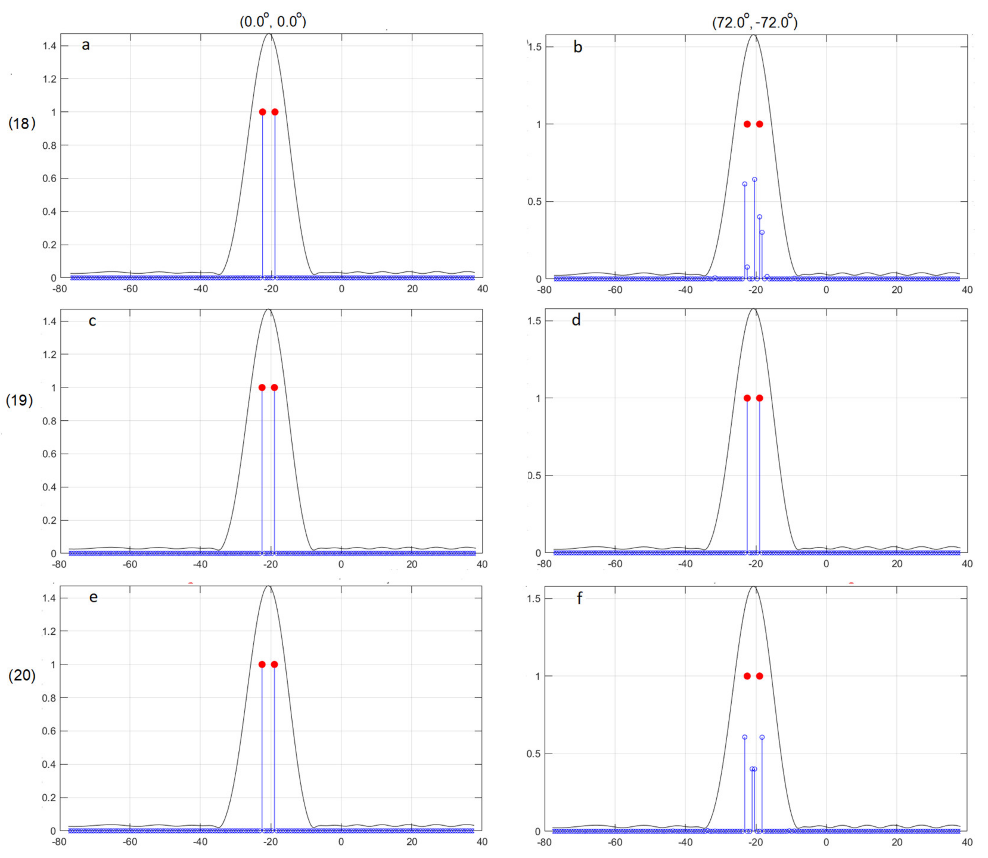
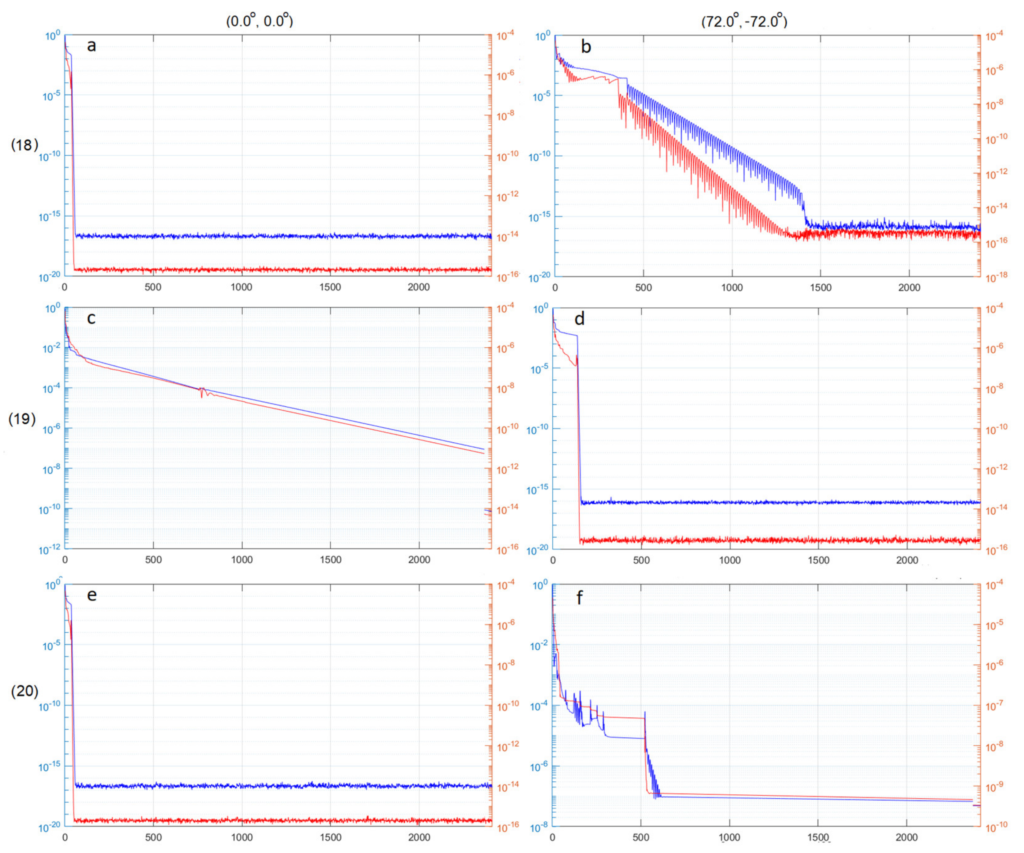
5.2. The Case of Two Sources with Different Initial Signal Phases

Next, Figure 4 and Figure 5 (similar to Figure 2 and Figure 3) show the results of a numerical simulation of the operation of a neural network with various activation functions (18)–(20) under the influence of two point sources with an amplitude of ${\dot{b}}_1={\dot{b}}_2=$1, angles of arrival of ${\theta }_1$ = −22.5° and ${\theta }_2=$ −18.98°, and two phase options for each of the two sources: ${\phi }_1$ = 0° and ${\phi }_2$ = 0°, and ${\phi }_1$ = 72° and ${\phi }_2$ = −72°.

In Figure 4 and Figure 5, the activation functions used from (18) to (20) are indicated vertically on the left, and at the top, horizontally, are the phase values used in modeling sources $({\phi }_1, {\phi }_2)$ = (0°, 0°) and $({\phi }_1, {\phi }_2)$ = (72°, −72°). For example, Figure 4c shows the plot obtained for the activation function (19) and the phases of sources ${\phi }_1$ = 0° and ${\phi }_2$ = 0°.

In Figure 4a–f, the angular directions in degrees are laid along the horizontal axis (in the grid of angular directions of an excessively complete basic dictionary); along the vertical axis are the values of the modules of the resulting basic components |X|, obtained as a result of processing using a neural network with the selected activation function. They correspond to the angular directions of the grid, the angles of the basic functions (blue), and the modules of the values of the radiation pattern |F|, formed in the same angular grid using the standard FFT method (black). The position of point sources, taking into account amplitudes ${\dot{b}}_1$and ${\dot{b}}_2,$is represented in red.

Figure 4. Two sources ${\dot{b}}_1={\dot{b}}_2=$ 1, ${\theta }_1$ = −22.5°, and ${\theta }_2=$ −18.98°, with values of |X| and |F|, activation functions (18)—subfigures (a,b), (19)—subfigures (c,d), (20)—subfigures (e,f).

Figure 4. Two sources ${\dot{b}}_1={\dot{b}}_2=$ 1, ${\theta }_1$ = −22.5°, and ${\theta }_2=$ −18.98°, with values of |X| and |F|, activation functions (18)—subfigures (a,b), (19)—subfigures (c,d), (20)—subfigures (e,f).

From the results obtained in all cases, the radiation pattern formed using FFT does not allow resolving sources at an angular distance between them equal to 3.52°. With a phase value of φ = (0°, 0°), all activation functions lead to an optimal solution with two non-zero basis coefficients, which correspond with the amplitude and direction of the sources (Figure 4a,c,e). However, like the case of one source, when a discrepancy occurs between the phases of the sources and the basis functions, the use of activation functions (18) and (20) leads to errors in determining the directions and amplitudes of the sources, as shown in Figure 4b,f. In this case, the number of non-zero values of the basic coefficients increases, and among them, there are no corresponding ones in the direction of the source.

Table 2. Number of basis coefficients with a level exceeding ${10}^{-3}$, two sources.

Activation Function	Source Phase	Coefficients Quantity
(18)	(0°, 0°)	2
(18)	(72°, −72°)	5
(19)	(0°, 0°)	2
(19)	(72°, −72°)	2
(20)	(0°, 0°)	4
(20)	(72°, −72°)	1

shows the number of basic coefficients with a value normalized to the maximum value $\underset{i}{\max }\left|x_i\right|$ exceeding ${10}^{-3}$.

In Figure 5a–f, the horizontal axis shows the time normalized to the duration of one internal calculation cycle t, and the vertical axis (scale on the left) shows the relative change in the coefficients of the basis functions for one normalized time step, $\mathsf{\Delta }X\left(t\right)=\underset{i}{\max }\left|x_i\left(t-1\right)-x_i\left(t\right)\right|/\underset{i}{\max }\left|x_i\left(t-1\right)\right|, t=1,2,\dots ,T$ (blue), and the current error in representing the input data by basis components, which was defined as the change in time of the loss function (6), as shown in the scale on the right (red).

Figure 5. Two sources ${\dot{b}}_1={\dot{b}}_2=$ 1, ${\theta }_1$ = −22.5°, and ${\theta }_2=$ −18.98°, with values of Δ|X(t)| and J(t), activation functions (18)—subfigures (a,b), (19)—subfigures (c,d), (20)—subfigures (e,f).

Figure 5. Two sources ${\dot{b}}_1={\dot{b}}_2=$ 1, ${\theta }_1$ = −22.5°, and ${\theta }_2=$ −18.98°, with values of Δ|X(t)| and J(t), activation functions (18)—subfigures (a,b), (19)—subfigures (c,d), (20)—subfigures (e,f).

From the results obtained, it follows that the time to establish the values of the coefficients of the basis functions when using activation functions (18) and (19) weakly depends on the value of the source phase.

For activation functions (18) and (20), it is clear that with phase values $({\phi }_1, {\phi }_2)$ = (72°, −72°), the process was unable to converge to a global minimum according to the l₀ norm, that is, to minimize the number of non-zero basic coefficients, although the loss function (6), for all options, was less than ${10}^{-9}$ and practically did not change over time, which indicates that the minimum in the l₁ norm has been reached. Thus, like the case of using activation functions (18) and (20) and phase φ = 72°, the value of the loss function (6) turned out to be very small, but the non-zero basis coefficients were very different from the source. In addition, the convergence process slowed down. Activation function (19), unlike the previous ones, made it possible to achieve a global minimum according to the l₀ norm, with an increase in time, in the cases considered, by 2–3 times.

An example of a change in the number of non-zero basis coefficients over time is presented in Figure 6. The number of basis coefficients is plotted along the vertical axis, and normalized time is plotted along the horizontal axis. The number of base coefficients is shown in different colors, the values of the modules of which, normalized to the maximum value $U=\left|X\left(t\right)\right|/\underset{i}{\max }\left|X\left(t\right)\right|$, exceed the following specified levels: [${10}^{-14}$,${10}^{-9}$, ${10}^{-4}$,${10}^{-3}$,${10}^{-2}$, ${10}^{-1}$]. (The legend is shown in the figure.)

It can be seen that all the basic coefficients quickly tend to become zero, and, in the end, in addition to the two basic coefficients corresponding to the source data, there are only three more coefficients with a level exceeding ${10}^{-9}$.

Thus, like the case with a single source, all three versions of the activation functions (18)–(20) allow, at zero initial phases, the accurate representation of the data with basis functions; however, if the initial phases of the sources are not zero, then options (18) and (20) may give a result that does not correspond to their real position and amplitude. The variant of activation function (19) for the considered case, as well as for a single source, demonstrated resistance to phase changes.

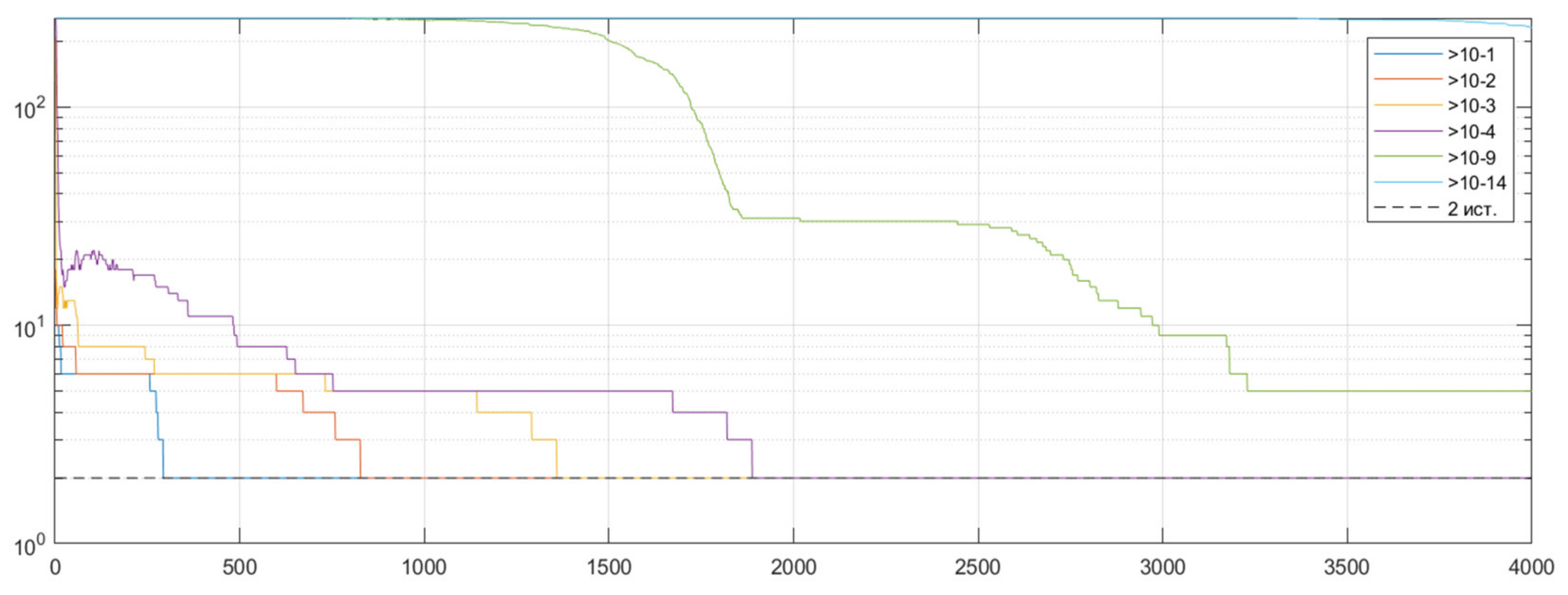
5.3. A Large Number of Sources

The following is the result of an analysis of the influence of the number of sources, which varied from 7 to 16, on the results of the MFNN neural network for complex data with the activation function (19), which showed the best result.

In Figure 7a,c,e, on the graphs, the horizontal axis shows the angular direction in degrees, and the vertical axis shows the values of the modules of the coefficients of the basis components X obtained at different times. They were obtained as a result of processing using a neural network with activation function (19), corresponding to the angular directions of the grid of angles of basis functions, as shown along the horizontal axis (blue lines), and the modules of the radiation pattern formed using FFT (black lines). The position of point sources, considering amplitudes ${\dot{b}}_i$and angles ${\theta }_i$, is represented by red dots.

In Figure 7a–f, the results are shown for the case of seven external sources, with levels ${\dot{b}}_{1-7}=$ [1.0, 1.0, 0.5, 2.0, 0.7, 1.0, 1.0] and angular directions ${\theta }_{1-7 }$ = [−42.19°, −33.75°, −22.50°, −18.98°, −11.25°, −5.63°, −2.11°] for the next three normalized time intervals T = [0–1000 ((a), (b)), 500–5000 ((c), (d)), 140,500–148,000 ((e), (f))], which show how the X coefficients and loss functions change (6). It can be seen that the X coefficients group quickly enough around the directions of the sources, and the values of the coefficients outside these zones drop below ${10}^{-8}$ (Figure 7a). If attention is paid to the graphs (Figure 7b,d,e), you can see that loss function (6) changes unevenly in jumps, while the changes in the basic coefficients remain generally monotonic. Subsequently, the process of changing the coefficients X slows down significantly, but their grouping continues in such a way that each direction to the source corresponds to its own area of significant coefficients, separated by zero coefficients from the rest (Figure 7c,e). By the time T = 148,000, there are only 16 significant basis coefficients of X, and only 10 of them have a value greater than ${10}^{-1}$. It turns out that in fact, the sums of the coefficients in these areas are equal to the levels of the corresponding sources, and the weighted average values of the angular directions in these areas are very close to the directions of the sources. The directions and levels determined in this way are displayed in Figure 7a,c,e with red dotted lines, which show the coincidence with the directions and levels of external sources. This feature makes it possible to significantly reduce the time required to find a solution to the system of differential Equation (14). Almost upon completion of the interval T = [0–1000] (Figure 7a), a result similar to that obtained in the interval T = [140,500–148,000] (Figure 7e) is achieved.

The graphs shown in Figure 8a,b are similar to those shown in Figure 7a, except the number of external sources for Figure 8a was 15: ${\dot{b}}_{1-15}=$ [1.0, 1.0, 0.5, 2.0, 0.7, 1.0, 1.0, 1.0, 0.5, 1.0, 1.0, 0.7, 0.8, 0.5, 1.0], and ${\theta }_{1-15 }$= [−42.19°, −33.75°, −22.50°, −18.98°, −11.25°, −5.63°, −2.11°, 5.63°, 9.14°, 16.88°, 19.69°, 28.13°, 31.64°, 39.36°, 47.81°]; for Figure 8b—16, another external source was added: ${\dot{b}}_{16}=$1.0, ${\theta }_{16 }$= 53.44°.

When exposed to 15 external sources (Figure 8a), the basis coefficients are concentrated around the directions to the sources, as noted above. Using the method of summing the coefficients in these areas and determining the angular directions from the weighted average values, similar to the previous one, it is possible to separate all external sources, except for the pair with coordinates at 16.88° and 19.69°, and determine their angular directions, in contrast to the case of using the FFT-based diagram formation. At the same time, when the number of external sources reaches 16, that is, it becomes equal to the number of ULA channels (Figure 8b), ten external sources cannot be resolved, although the tendency of grouping around the directions to the sources remains.

6. Conclusions

The article discusses the proposed implementation of a sparse representation of complex data based on an overcomplete basis, l₀/l₁ norms, and a neural-like MFNN [19,20,21] for the case of complex data. It is shown that the modification of the initializing function of a neural network proposed in the article allows one to effectively solve the problem of representing complex data by elements of a complex basis. The influence of the choice of the type of initializing function on the characteristics of the neural network is analyzed. It is shown that the initializing function (19) is optimal if the phases of these sources and the selected complex overcomplete basis are different. In relation to the problem of determining the direction to the sources of signals received by a linear antenna array, a significant increase in the resolution in angular direction was demonstrated in comparison with the classical processing method based on the FFT algorithm. Unlike SL0 [21], this is guaranteed to converge with the optimal solution but shows a slower rate of convergence.

In subsequent studies, there are plans to conduct a detailed analysis of methods for accelerating the convergence of the method under consideration, as well as an experimental study of its characteristics for processing multidimensional data.

References

1. Schmidt, R.O. Multiple Emitter Location and Signal Parameter Estimation. IEEE Trans. Antennas Propag. 1986, 34, 276–280. [Google Scholar] [CrossRef]
2. Rao, B.D.; Hari, K.V.S. Performance analysis of root-MUSIC. IEEE Trans. Acoust. Speech Signal Process. 1989, 37, 1939–1949. [Google Scholar] [CrossRef]
3. Zala, C.A.; Barrodale, I.; Kennedy, J.S. High-resolution signal and noise field estimation using the L1 (least absolute values) norm. IEEE J. Ocean. Eng. 1987, 12, 253–264. [Google Scholar] [CrossRef]
4. Bandler, J.W.; Kellerman, W.; Madsen, K. A nonlinear L1 optimization algorithm for design, modeling, and diagnosis of networks. IEEE Trans. Circuits Syst. 1987, 34, 174–181. [Google Scholar] [CrossRef]
5. Abdelmalek, N.N. Solutions of minimum time problem and minimum fuel problem for discrete linear admissible control systems. Int. J. Syst. Sci. 1978, 8, 849–859. [Google Scholar] [CrossRef]
6. Levy, S.; Walker, C.; Ulrych, T.J.; Fullagar, P.K. A linear programming approach to the estimation of the power spectra of harmonic processes. IEEE Trans. Acoust. Speech Signal Process. 1992, 30, 675–679. [Google Scholar] [CrossRef]
7. Stanković, L.; Sejdić, E.; Stanković, S.; Daković, M.; Orović, I. A Tutorial on Sparse Signal Reconstruction and Its Applications in Signal Processing. Circuits Syst. Signal Process. 2019, 38, 1206–1263. [Google Scholar] [CrossRef]
8. Zhang, Y.; Xiao, S.; Huang, D.; Sun, D.; Liu, L.; Cui, H. L0-norm penalized shrinkage linear and widely linear LMS algorithms for sparse system identification. IET Signal Process. 2017, 11, 86–94. [Google Scholar] [CrossRef]
9. Ishii, Y.; Koide, S.; Hayakawa, K. L0-norm Constrained Autoencoders for Unsupervised Outlier Detection. In Advances in Knowledge Discovery and Data Mining. PAKDD 2020; Lauw, H., Wong, R.W., Ntoulas, A., Lim, E.P., Ng, S.K., Pan, S., Eds.; Lecture Notes in Computer Science; Springer: Cham, Switzerland, 2020; Volume 12085. [Google Scholar] [CrossRef]
10. Marquardt, D.W.; Snee, R.D. Ridge regression in practice. Am. Stat. 1975, 29, 3–20. [Google Scholar] [CrossRef]
11. Rajko, R. Studies on the adaptability of different Borgen norms applied in selfmodeling curve resolution (SMCR) method. J. Chemom. 2009, 23, 265–274. [Google Scholar] [CrossRef]
12. Tibshirani, R. Regression shrinkage and selection via the lasso. J. R. Stat. Soc. B 1996, 58, 267–288. [Google Scholar] [CrossRef]
13. Schmidt, R.O. A Signal Subspace Approach to Multiple Emitter Location and Spectral Estimation. Ph.D. Thesis, Stanford University, Stanford, CA, USA, 1981. [Google Scholar]
14. Capon, J. High resolution frequency-wavenumber spectrum analysis. Proc. IEEE 1969, 57, 1408–1418. [Google Scholar] [CrossRef]
15. Sun, K.; Liu, Y.; Meng, H.; Wang, X. Adaptive Sparse Representation for Source Localization with Gain/Phase Errors. Sensors 2011, 11, 4780–4793. [Google Scholar] [CrossRef] [PubMed]
16. Donoho, D.L.; Huo, X. Uncertainty Principles and Ideal Atomic Decomposition. IEEE Trans. Inf. Theory 2001, 47, 2845–2862. [Google Scholar] [CrossRef]
17. Malioutov, D.M.; Cetin, M.; Willsky, A.S. Optimal sparse representations in general overcomplete bases. In Proceedings of the 2004 IEEE International Conference on Acoustics, Speech, and Signal Processing, Montreal, QC, Canada, 17–21 May 2004. [Google Scholar] [CrossRef]
18. Cichocki, A.; Unbehauen, R. Neural Networks for Solving Systems of Linear Equations and Related Problems. IEEE Trans. Circuits Syst. I Fund. Theory Appl. 1992, 39, 124–138. [Google Scholar] [CrossRef]
19. Wang, Z.S.; Cheung, J.Y.; Xia, Y.S.; Chen, J.D.Z. Minimum fuel neural networks and their applications to overcomplete signal representations. IEEE Trans. Circuits Syst. I Fund. Theory Appl. 2000, 47, 1146–1159. [Google Scholar] [CrossRef]
20. Kümmerle, C.; Verdun, C.M.; Stöger, D. Iteratively Reweighted Least Squares for Basis Pursuit with Global Linear Convergence Rate. In Proceedings of the Advances in Neural Information Processing Systems 34 (NeurIPS 2021), Online, 6–14 December 2021; Volume 34, pp. 2873–2886. [Google Scholar]
21. Mohimani, G.H.; Babaie-Zadeh, M.; Jutten, C. Complex-valued sparse representation based on smoothed l0 norm. In Proceedings of the IEEE International Conference on Acoustics, Speech and Signal Processing, Las Vegas, NV, USA, 31 March–4 April 2008; pp. 3881–3884. [Google Scholar] [CrossRef]
22. Mohimani, H.; Babaie-Zadeh, M.; Jutten, C. A fast approach for overcomplete sparse decomposition based on smoothed l0 norm. IEE Trans. Signal Process. 2009, 57, 289–301. [Google Scholar] [CrossRef]
23. Wang, L.; Yin, X.; Yue, H.; Xiang, J. A regularized weighted smoothed L0 norm minimization method for underdetermined blind source separation. Sensors 2018, 12, 4260. [Google Scholar] [CrossRef] [PubMed]
Figure 1. Neural network architecture for M = 8 and N = 3 [19].
Applsci 14 01959 g001
Figure 3. Single external source b ˙ 1 =  1, θ 1 = −22.5°, with values of Δ|X(t)| and J(t), activation functions (18)—subfigures (a,d,g), (19)—subfigures (b,e,h), (20)—subfigures (c,f,i).
Applsci 14 01959 g003
Figure 6. Two sources b ˙ 1 = b ˙ 2 =  1, θ 1 = −22.5°, and θ 2 = −18.98°; number of basis coefficients for U > [ 10 14 ,   10 9 , 10 4 ,   10 3 ,   10 2 , 10 1 ].
Applsci 14 01959 g006
Figure 7. Seven sources b ˙ 1 7 = [1.0, 1.0, 0.5, 2.0, 0.7, 1.0, 1.0], and θ 1 7   = [−42.19°, −33.75°, −22.50°, −18.98°, −11.25°, −5.63°, −2.11°], with values of |X|, Δ|X(t)|, and J(t), the interval T = [0–1000] subfigures (a,b), T = [1300–5000] subfigures (c,d), T = [140,500–148,000] subfigure (e,f).
Applsci 14 01959 g007
Figure 8. Fifteen (a) and sixteen (b) external sources, with values of |X|.
Applsci 14 01959 g008