High-Dimensional Ensemble Learning Classification: An Ensemble Learning Classification Algorithm Based on High-Dimensional Feature Space Reconstruction

Abstract

When performing classification tasks on high-dimensional data, traditional machine learning algorithms often fail to filter out valid information in the features adequately, leading to low levels of classification accuracy. Therefore, this paper explores the high-dimensional data from both the data feature dimension and the model ensemble dimension. We propose a high-dimensional ensemble learning classification algorithm focusing on feature space reconstruction and classifier ensemble, called the HDELC algorithm. First, the algorithm considers feature space reconstruction and then generates a feature space reconstruction matrix. It effectively achieves feature selection and reconstruction for high-dimensional data. An optimal feature space is generated for the subsequent ensemble of the classifier, which enhances the representativeness of the feature space. Second, we recursively determine the number of classifiers and the number of feature subspaces in the ensemble model. Different classifiers in the ensemble system are assigned mutually exclusive non-intersecting feature subspaces for model training. The experimental results show that the HDELC algorithm has advantages compared with most high-dimensional datasets due to its more efficient feature space ensemble capability and relatively reliable ensemble operation performance. The HDELC algorithm makes it possible to solve the classification problem for high-dimensional data effectively and has vital research and application value.

1. Introduction

Various multi-dimensional heterogeneous data, such as low signal-to-noise ratio, can be collected through simultaneous access to information sources and used to comprehensively solve classification problems. For example, in gene expression [1] data, each sample may contain the expression levels of thousands of genes, which will be used as features for disease diagnosis, drug-response classification prediction, and other studies. In financial analysis [2], the basic features of each stock include opening price, closing price, high price, low price, volume, etc., and also have features such as macroeconomic indicators, company fundamental information, etc., which are used to construct complex stock market classification prediction models. Multiple data such as physiological signal data (heart rate, blood pressure, blood glucose level), electronic health records, diagnostic records, medication usage records, etc., are involved in the health and disease screening task [3], and data such as air quality sensor data, water quality monitoring data, meteorological data, and satellite remote sensing data are acquired through multiple sensors in an environmental monitoring [4] classification task. How to fully extract valid and interpretable information from these high-dimensional data has become a hot topic widely studied by scholars nowadays. Another issue is too much redundant information and the insufficient extraction of crucial information. This kind of high dimensional data with different independence and relevance increases the difficulty of information search and model matching and leads to poor classification results.

Ensemble learning [5,6,7] algorithms can combine a variety of typical conventional classifiers organically and overcome the limitations of traditional single classifiers for high-dimensional-data classification tasks. The overall ensemble model is built by fully using various valid information regarding high-dimensional data. It can improve the robustness and generalization performance of the learning model. Many ensemble learning algorithms have been proposed in recent years, such as bagging [8], random forest [9], a fuzzy classifier ensemble [10,11], and a neural network-based classifier ensemble [12,13].

However, most ensemble algorithms are implemented directly on the original feature space, which must be revised in classification tasks for high-dimensional data with redundancy and noise. For sample space-based Adaboost algorithms [14], they do not provide substantial diversity for high-dimensional data containing redundancy; for feature space-based methods, such as random subspace algorithms [15], they do not provide effective filtering for high-dimensional features, and fusion on subspaces can lead to information loss and degrade classifier performance. Therefore, for high-dimensional data, although traditional integrated learning algorithms can accomplish the data classification task better, they still have the following shortcomings: 1. Simple math-driven methods make it difficult to compress the high-dimensional-data space, which makes it challenging to construct an accurate and reliable classification model. 2. Considering feature selection and model integration separately and independently will lead to the low robustness and scalability of the task of high-dimensional data.

In order to overcome the above limitations, we propose a high-dimensional ensemble learning classification algorithm based on feature space reconstruction, called HDELC algorithm (HDELC is the abbreviation of high-dimensional ensemble learning classification), which selects and combines features more intelligently through feature space reconstruction to reduce dimensionality effectively instead of applying simple mathematical compression techniques on high-dimensional data, and retain the information crucial to the classification task. It focuses on data feature space and model integration, which can improve the diversity of models and accuracy in learning high-dimensional data to a certain extent.

Precisely, the HDELC algorithm first reconstructs the original feature space, establishes the feature space reconstruction matrix through the two thresholds of the mean value of information entropy and the screening factor of feature attributes, splits the original feature space, and obtains the optimal feature space scale. Based on the optimal feature space scale, PCA is used to downscale the original feature space to obtain a new high-dimensional feature reconstruction space. The high-dimensional feature reconstruction space is defined as the set of solid feature spaces divided by the average information entropy and the set of optimal weak feature spaces preserved by the screening coefficients. The scale of this feature space is the dimension to which the PCA downscaling needs to be reduced. The feature subspace is a smaller set of features chosen from the original feature space; the set of feature subspaces after dimensionality reduction is used as the best feature subspace and as the feature set for subsequent subspace integration work. Secondly, based on the Stacking model [16], the feature space is divided into several mutually exclusive non-intersecting feature subspaces to determine the optimal number of classifiers in the integrated system to achieve the goal of the overall integration model: “good but different”. “Good but different” means that by assigning different feature subspaces to different classifiers, the performance of the integrated model is improved while ensuring the diversity of classifiers in the integrated system.

The contributions of this paper are twofold. Firstly, it focuses on exploring helpful information in the feature space of high-dimensional data and proposes a high-dimensional feature space reconstruction strategy based on the feature space (partition) selection matrix; secondly, a selective subspace ensemble algorithm is designed to optimize the ensemble model and ensure model accuracy and diversity.

The rest of the paper is organized as follows. Section 2 introduces some preliminary knowledge of integration learning in previous work related to high-dimensional data ensemble models; Section 3 details the specific process of the high-dimensional data ensemble classification algorithm (HDELC algorithm) based on the reconstruction and ensemble of high-dimensional feature space; Section 4 evaluates the performance of our proposed model through comparative experiments and ablation experiments; and Section 5 summarizes the work of this paper, provides a summary future work and the outlook of the future work.

2. Related Work

Ensemble learning (EL) is an advanced machine learning technique that aims to improve model accuracy, stability, and generalization by combining the predictive power of multiple learners (also known as models). The technique is based on the core premise that integrating multiple models can produce superior predictive performance than a single model. By integrating the classification predictions from multiple models, integrated learning can capture more complex patterns and relationships in the data and thus demonstrate more robust generalization capabilities on unseen data.

Integrated learning techniques have been widely used in several practical application scenarios and have achieved significant results, such as financial risk assessment, image recognition, speech recognition, and natural language processing, etc., which can synthesize multiple models to adapt to the complexity of the data and achieve significant performance improvement in multiple tasks.

A large number of excellent approaches have been proposed by scholars for the classification problem of high-dimensional data.

Some studies focus on feature data selection by proposing a new feature dimensionality reduction strategy for data lacking sparsity and interpretability, and then, iteratively compute the model performance using mainstream classifiers to obtain the final classification results.

For example, Xiaomeng Li et al. [17] performed dimensionality reduction on monitoring data of mechanical conditions, introduced an autoencoder to mine the degraded feature space, and provided a comprehensive representation of the degraded data in different aspects, which verified the model validity. Jayaraju Priyadarshini et al. [18] employed six physically inspired metaphorical algorithms for a K-nearest-neighbor analysis of feature selection, and the accuracy was about 8% higher than the meta-heuristic-algorithm approach. Li Y et al. [19] proposed a framework for joint dimensionality reduction and dictionary learning, using self-encoders to learn the non-linear mapping of the feature space and optimizing the model performance through the mapping function and dictionary simultaneously, and experimentally verified the effectiveness of the proposed model. Wang Q et al. [20] first used both eigenvalue search and subspace sampling to process high-dimensional data, and then designed an efficient random forest algorithm. Experimental tests using the face dataset, the experimental results show that this algorithm can guarantee prediction accuracy while significantly reducing the prediction error compared with existing random forest algorithms with an accuracy of 95.7%. Khandaker Mohammad Mohi Uddin et al. [21] developed a machine learning-based CAAD algorithm to explore hyper-parameter tuning with feature scaling and optimization strategies, which resulted in up to 98.77% accuracy of voting classifier in a breast cancer diagnosis task and validated the effectiveness of the model.

Some algorithms focus on constructing a new ensemble learning model to improve the model’s generalization performance and classification accuracy. They theoretically explore and analyze the nature of the classifier ensemble and can improve the ensemble learning algorithm framework and the model’s generalization ability.

Stéphane Cédric Koumétio Tékouabou et al. [22] improved the model performance by combining integration methods such as bagging classifiers (BCs) with dynamic/static selection strategies (BC-DS/SS) in three-stage fusion. Che Xu et al. [23] considered the individual accuracies of the base classifiers (BCs) and the diversity among classifiers and proposed a sequential instance selection framework based on genetic algorithms. They verified the ability of the proposed framework to improve the convergence performance compared with six benchmark integration learning methods. Kurutach T et al. [24] used a model-ensemble trust-region policy optimization (ME-TRPO) strategy to integrate the model, ensuring uncertainty in the model and regularizing the training process. Ahmed K et al. [25] proposed a multi-model fusion strategy (MME) based on KNN and RVM for the predictive classification task of weather data, and this strategy was able to determine the optimal number of circulation models from a set of circulation models. Zhong Y et al. [26] first set a dynamic threshold. They ensemble multiple learners under the threshold constraint to propose the HELAD ensemble algorithm, and this ensemble framework can achieve better competitiveness and accuracy in anomaly detection tasks for network traffic.

Although these algorithms can improve the model performance compared to traditional ensemble learning algorithms, most ensemble learning algorithms consider sample space and feature space separately. On the other hand, ensemble learning systems do not need to select all base learners for the ensemble, and some researchers suggest choosing the appropriate learners to achieve better classification performance.

Although the ensemble learning strategy uses multiple classifiers to improve the model generalization performance, it alleviates the limitation that training the optimal classifier on high-dimensional data is challenging. However, most studies either perform dimensionality reduction on features but do not assign proper classifiers to them, or, alternatively, only a base classifier ensemble with diversity is considered and implemented directly on the original feature space, and it is susceptible to noise and redundant features.

Therefore, these methods still have limitations when faced with classification tasks for high-dimensional data:

(1)

Most of the above feature selection algorithms are designed to obtain an optimal subset of features. In contrast, the classifier calls an existing subset of features and uses a fixed structure when evaluating the subset of features. Therefore, the classifier used may not be the best.

(2)

Different classifiers, such as decision trees, support vector machines (SVMs), etc., based on their unique learning algorithms, will produce different predictions on the same dataset. These differences arise from the different ways in which individual algorithms partition the feature space of the data and the trade-offs they make between model complexity, bias, and variance. In a numerical analysis, this prediction variability can lead to a significant impact on the overall prediction results of the integrated model.

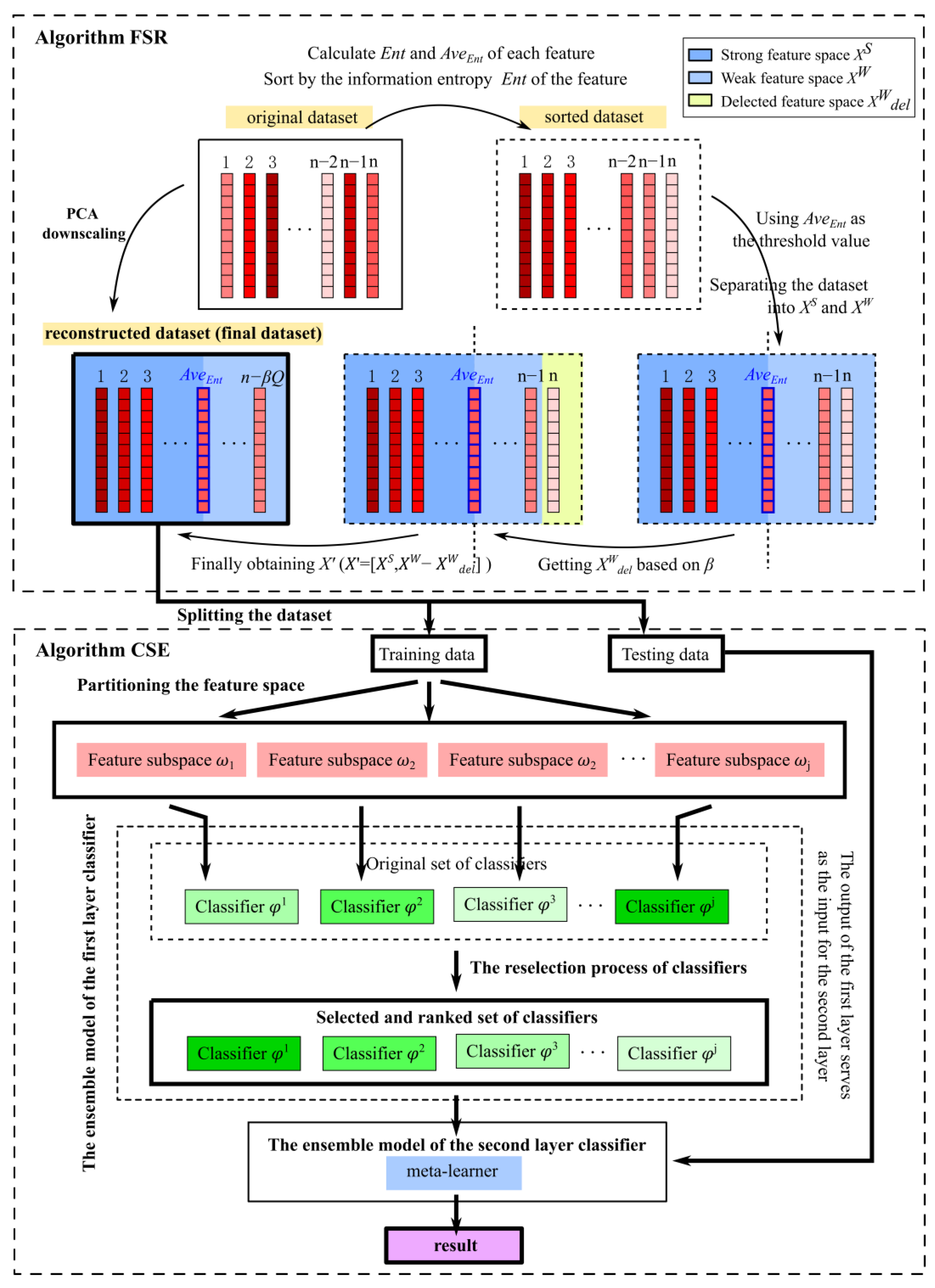
3. HDELC Algorithm

The high-dimensional ensemble learning classification algorithm (HDELC algorithm) can improve the model’s performance by using both global and local structural information of high-dimensional data. Specifically, it is divided into two significant aspects. Firstly, the data feature space is processed. The feature space is divided into multiple local feature regions by constructing a threshold and feature reconstruction matrix. Second, the model is trained using several single classifiers and subspace ensemble methods within different local feature regions. The prediction results between different feature space regions use ensemble to obtain more accurate prediction results. Figure 1 shows the flow chart of the HDELC algorithm based on the feature space reconstruction matrix.

Given a training set, $M=\left\{\left(x_1,y_1\right),\left(x_2,y_2\right),\dots ,\left(x_L,y_L\right)\right\}$ with $L$ samples, where $x_i\left(i\in \left\{1,2,\dots , L\right\}\right)$ is the training sample, $y_i\left(i\in \left\{1,2,\dots ,k\right\}\right)$ is the label of the ith training sample, k is the number of classes, and each sample $x_i\in \left\{x_{i1},x_{i2},\dots ,x_{in}\right\}$ consists of $n$ features. $\widehat{\phi }=\left\{{\phi }^1,{\phi }^2,\dots ,{\phi }^H\right\}$ denotes all classifiers in the ensemble model. (See Algorithm 1).

Algorithm 1. Subspace ensemble strategy based on high-dimensional feature space reconstruction.

Require: Input: Original high-dimensional dataset. Procedure 1: Obtain the optimal feature space with Algorithm 2; 2: Find the feature-reconstructed dataset (final dataset); 3: Spilt the reconstructed dataset into training data and testing data; 4: Train the $\widehat{\phi }=\left\{{\phi }^1,{\phi }^2,\dots ,{\phi }^H\right\}$ using the training data; 5: Sort the training results for each classifier; 6: Divide feature subspaces; 7: Select the classifiers in the ensemble model using the Algorithm 3; 8: Build the first layer of the ensemble training model; 9: Train the model using the model prediction results as input to the second-layer learner. Output: Predicted results of the HDELC model.

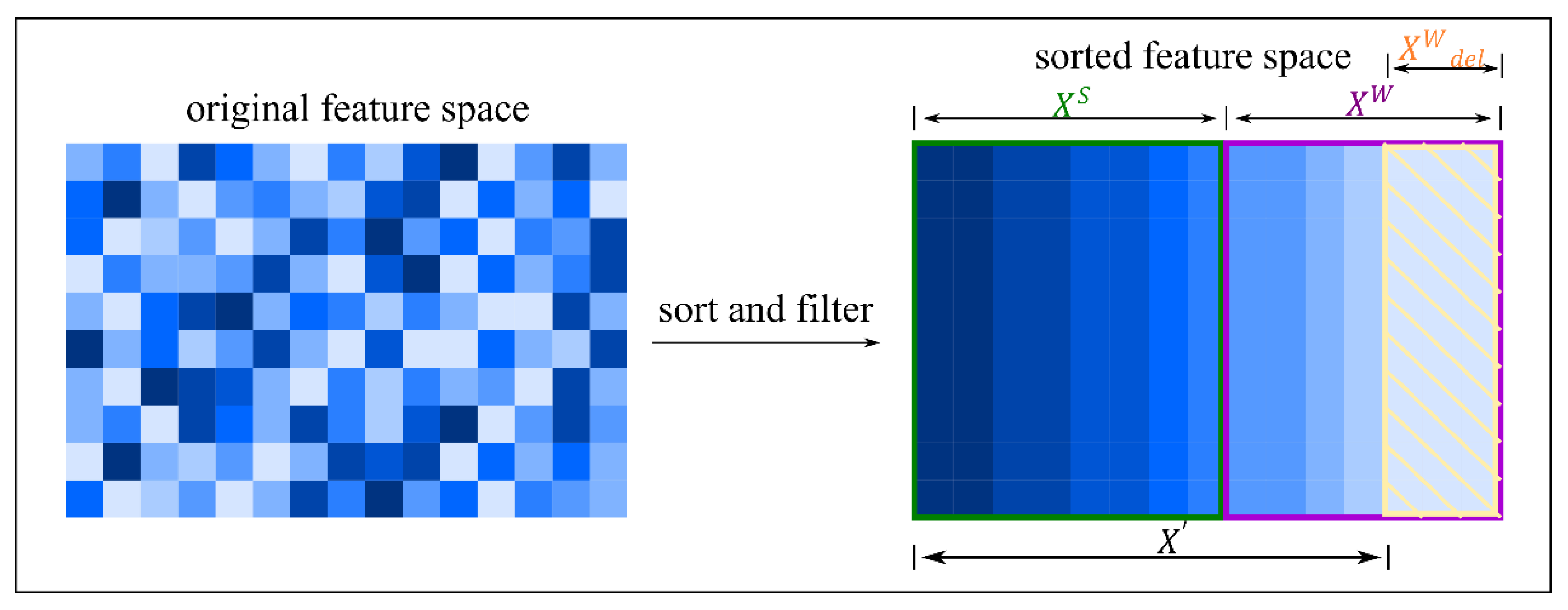
3.1. High-Dimensional Feature Space Reconstruction Process

Reconstructing the high-dimensional feature space can maximize model diversity and local optimization performance. It divides the original high-dimensional data into relatively independent subsets of different feature spaces. Not only can the correlation between individual base classifiers be reduced, but also the operations are executed relatively faster due to the reduced size of the input feature space corresponding to each base classifier. The algorithmic flow of high- dimensional feature space reconstruction is given using the FSR algorithm (the abbreviation of feature subspace reconstruction strategy).

Algorithm 2. Feature subspace reconstruction strategy

Require: Input: The feature space selection matrix $X$; Procedure 1: For $i$ in $1,\dots ,n$; 2: Calculate the information entropy $Ent\left(x_i\right)$; 3: Calculate the average value of information entropy $Av{e}_{Ent}$; 4: if $Ent\left(x_i\right)\le Av{e}_{Ent}$ 5:  Place $x_i$ in the set $X^S$; 6: Or; 7:  Place $x_i$ in the set $X^W$; 8: Set the filter factor $\beta$; 9: Calculate the number of features $\left|{X^W}_{del}\right|$ that are rejected in weak feature space; 10: Redivide and the weak feature space $X^W$; 11: Refactor the feature space $X^{\prime }$; 12: Use $X^{\prime }\in \left({X_1}^{\prime },{X_2}^{\prime },\dots ,{X_B}^{\prime }\right)$ to train the decision tree classifier $\left({\phi }_1,{\phi }_2,\dots ,{\phi }_B\right)$; 13: Select the attribute screening factor corresponding to the maximum precision as the optimal attribute screening factor, and then determine the optimal feature selection set size $\left|X^{best}\right|$; 14: Use PCA dimensionality reduction to reduce the original feature space $X$ to $\left|X^{best}\right|$ dimension. Output: The optimal feature selection set size $\left|X^{best}\right|$ and feature-reconstructed dataset.

For the reconstruction process of the high-dimensional feature space, first, the entropy weight method [27] is used to obtain the information entropy of each feature and its weight. In this way, the importance of the features is evaluated. The mean value of information entropy of all features is calculated and used as the threshold value. The construction of the feature space reconstruction matrix will be based on this threshold value.

Information entropy is directly related to the predictive uncertainty of the features, can provide an objective method to assess the contribution of the features, and can accurately quantify the uncertainty level of the features in the classification task. By measuring features with low information (i.e., high uncertainty) based on the information entropy mean, the complexity of the model can be effectively reduced, thereby reducing the risk of overfitting and improving the model’s generalization ability. Using the mean value of information entropy as the delineation boundary of feature importance, the set of features with information entropy that is more significant than the threshold value is considered for a partial optimization operation.

Second, the threshold value is used for feature importance classification. We optimize the set of features whose partial information entropy is more significant than the threshold value. In order to maximize the valuable information in the features and reduce the feature space size, the redundant features are discarded to load the model computation. We set the attribute screening factor $\beta$ as the screening coefficient for the set of features more significant than the threshold, $\beta \in \left[0.1,0.2,0.3,0.4,0.5\right]$, and perform a sensitivity analysis on it. The set of feature subspaces under each attribute rounding factor constraint is used to construct the feature space reconstruction matrix. When training on the samples, it is convenient to locate the target selected features quickly. A set of decision tree classifiers are trained using the set of feature subspaces under each attribute discard factor constraint. The features used for decision tree branching are selected by comparing the information gain [28] $\phi$ of different features. The information gain $\phi$ is defined as follows:

$$\phi \left(M,X\right)=Ent\left(M\right)-Ent(M|X)$$

(1)

$$Ent\left(M\right)=-{\displaystyle \sum }_{k=1}^K\frac{C_k}{M}{\log }_2\frac{C_k}{M}$$

(2)

$$Ent\left(M|X\right)=-{\displaystyle \sum }_{i=1}^m\frac{\left|M_i\right|}{\left|M\right|}{\displaystyle \sum }_{k=1}^K\frac{\left|M_{ik}\right|}{\left|M_i\right|}{\log }_2\frac{\left|M_{ik}\right|}{\left|M_i\right|}$$

(3)

where $\phi \left(M, X\right)$ is the information gain of feature $X$ on the training dataset $M$, $Ent\left(M\right)$ is the empirical entropy of the dataset $M$, and $Ent\left(M|X\right)$ is the empirical conditional entropy of feature $X$ on the dataset $M$. The sample size of dataset $M$ is $\left|M\right|$, $k$ is the number of classification labels, $\left|C_k\right|$ is the number of samples belonging to category $C_k$, ${{\displaystyle \sum }}_{k=1}^K\left|C_k\right|=\left|M\right|$. The values of feature $X$ are $a_1,a_2,\dots , a_m$, and according to the values of $A$, $M$ is divided into $m$ subsets $M_1, M_2,\dots , M_m$. $\left|M_i\right|$ is the number of samples of $M_i$, ${{\displaystyle \sum }}_{i=1}^m\left|M_i\right|=\left|M\right|$. The set of samples belonging to $C_k$ in the feature subset $M_i$ is $M_{ik}$, $\left|M_{ik}\right|$ is the number of samples of $M_{ik}$.

For each node of the decision tree, the information gain of each feature is calculated, and the maximum information gain feature is selected as the basis for splitting the nodes. After branching continuously recursively, all training samples are assigned to the child nodes according to the branching condition. The feature space size corresponding to the feature space matrix under the constraint of the optimal attribute screening factor is the optimal feature selection set size.

Finally, since the PCA dimensionality reduction method can filter the noisy data, while retaining the essential features, the number of features corresponding to the optimal feature selection set size is used as the basis for PCA dimensionality reduction to optimize the size of the original feature space, which ensures the rigor of the dimensionality reduction scale as well as ensures that the original information is not lost. The optimized original feature space is used for subsequent research of classifier integration.

3.1.1. Construction of the Feature Space Reconstruction Matrix

In order to solve the problem that high-dimensional data will reduce the model’s computational efficiency in the model training process, it is necessary to select the feature domain before training the high-dimensional data model. The features with high relative importance are selected as feature subsets for classifier training. The optimal subset size of the feature space is selected through the construction of the feature selection space matrix. It can retain the valuable information in the original data as much as possible in the feature selection stage and improve the efficiency and accuracy of the model operation.

Suppose that the input of the decision tree is the training dataset $M$ with the number of samples $\left|M\right|$, and $z=\left[z_1,z_2,\dots ,z_n\right]$ represents a sample in the dataset of dimension $n$. Meanwhile, X is the matrix representing the training dataset with size $l$ rows and $n$ columns, $Y$ is the label vector of the training dataset with length $l$, and $Y={\left[y_1,y_2,\dots ,y_l\right]}^T$.

In the feature selection phase, the information entropy of each feature is first calculated, and the features in the original feature space are arranged in ascending order according to the information entropy. Information entropy was introduced by Claude Shannon in 1948 to quantify the uncertainty or average content of information in a source. In the concept of information theory, assuming that a source given using a discrete random variable $X=\left\{x_1,x_2,\dots ,x_n\right\}$ has a probability of occurrence $p_i=P\left(x_i\right)\left(i=1,2,\dots ,n\right)$ and ${{\displaystyle \sum }}_{i=1}^n{p}_i=1$, the information entropy of the source $X$ is expressed as

$$Ent\left(x_i\right)={\displaystyle \sum }_{i=1}^n{p}_i{\log }_2\frac{1}{p_i}=-k{\displaystyle \sum }_{i=1}^n{p}_i\ln p_i$$

(4)

where $Ent\left(x_i\right)$ is the characterization quantity for the overall characteristics of the source, it is a measure of the uncertainty of the source metric output information and the randomness of event occurrence.

In classifier integration, especially when using gradient boosting methods (e.g., gradient boosting trees) for model training, information entropy based on natural logarithms can simplify gradient computation. Moreover, the derivative of the natural logarithm has a concise form, which helps to compute the gradient and perform effective optimization. For using natural logarithms to represent information entropy, where $k={\log }_{2}e,$ we use the Boltzmann constant [29].

Based on the information entropy of each feature, calculate its corresponding coefficient of variability ${\alpha }_i$ and weight ${\gamma }_i$ as follows.

$${\alpha }_i=1-Ent\left(x_i\right)$$

(5)

$${\gamma }_i=\frac{{\alpha }_i}{{{\displaystyle \sum }}_1^n{\alpha }_i}$$

(6)

The average information entropy $Av{e}_{Ent}$ of each feature is calculated and used as a basis for classifying the importance of features in the feature space, as shown in Equation (7):

$$Av{e}_{Ent}=\frac{{{\displaystyle \sum }}_1^{n}Ent\left(x_i\right)}{n}$$

(7)

At this point, the average information entropy is used as the feature space division threshold. This threshold divides the feature space into two major regions, with features with information entropy less significant than the average information entropy marked as $Av{e}_{Ent}$ and features with information entropy higher than average marked as $Av{e}_{Ent}$ and weak features, as follows:

$$x_i=\{\begin{array}{c}strong feature\left(x_i>Av{e}_{Ent},x_i\in X\right)\\ weak feature\left(x_i<Av{e}_{Ent},x_i\in X\right)\end{array}$$

(8)

Strong features are often considered those with relatively low information entropy, meaning they exhibit significant regularity or certainty in the dataset. Low entropy features distinguish categories because they exhibit significantly different distribution patterns across categories or outcomes. Secondly, strong features contribute significantly to predicting or categorizing the target variable and can significantly improve the model’s performance. Such features usually contain information crucial for problem-solving and should be prioritized for retention in the feature selection process.

On the contrary, weak features tend to have high information entropy, indicating that they are more evenly distributed in the dataset, with roughly the same probability of occurrence for each state, which results in the features being less capable of distinguishing between different classes or outcomes. High entropy features may contain a large amount of noisy information and have limited contribution to the prediction of the target variable. Moreover, weak features contribute less to improving the model performance and even introduce errors that increase the model complexity without improving the prediction ability.

This results in a feature subspace $X^S$ consisting of strong features and a feature subspace $X^W$ consisting of weak ones. After that, the original feature space samples can be redefined after the average information entropy division as

$$X=\left[X\ast F_S,X\ast (I-F_S\right)]=[X^S,X^W]$$

(9)

where “$\ast$” is the product of the corresponding elements of the two matrices, i.e., the Hadamard product of the two matrices. $I$ is a unit matrix of $l$ rows and $n$ columns, and $F_S$ denotes the eigenspace reconstruction matrix obtained after the eigenspace has been partitioned using a threshold, which is a matrix of $l$ rows and $n$ columns, defined as follows:

$$F_S=\left[\begin{array}{cccc}{{\partial }_1}^1& {{\partial }_2}^1& \cdots & {{\partial }_n}^1\\ {{\partial }_1}^2& {{\partial }_2}^2& \cdots & {{\partial }_n}^2\\ \cdots & \cdots & \cdots & \cdots \\ {{\partial }_1}^l& {{\partial }_2}^l& \cdots & {{\partial }_n}^l\end{array}\right]$$

(10)

Of which,

$${{\partial }_i}^j=\{\begin{array}{c}1\left(i\in \left\{1,\dots ,n\right\},j\in \left\{1,\dots ,l\right\},x_i\in X^S\right)\\ 0\left(i\in \left\{1,\dots ,n\right\},j\in \left\{1,\dots ,l\right\},x_i\in X^W\right)\end{array}$$

(11)

Based on the division of the average information entropy, the feature space reconstruction matrix is established, the significance of which is able to divide the features with strong and weak feature information, obtaining a feature space reconstruction matrix consisting of 1 and 0, representing strong and weak features, respectively. It is also possible to observe the change in the importance of the feature space more clearly and to extract the selected feature space more quickly when the model is trained for classification.

3.1.2. Feature Subspace Division and Reconstruction Process

After constructing the feature space reconstruction matrix in the previous section, the attribute screening factor $\beta$ is set as the screening coefficient to optimize the number of features in the set of weak feature spaces (features more significant than the threshold), and the original feature space is partitioned twice, i.e., to the set of weak feature subspaces $X^W$ as follows:

$$\left|{X^W}_{del}\right|=\beta ·\left|X^W\right|$$

(12)

where “·” is the product of the screening factor and each element of the matrix, ${X^W}_{del}$ is the set of eliminated features in the set of weak feature space, $\left|{X^W}_{del}\right|$ is the number of eliminated features in the set of weak feature space $X^W$, $\left|X^W\right|$ is the number of features in the set of weak feature subspace $X^W$. The product of the attribute screening factor $\beta$ and the number of features $\left|X^W\right|$ in the weak feature subspace set $X^W$ is the number of features that will be screened and optimized in the weak feature subspace, which corresponds to the scale of PCA downscaling.

Let the number of features in the strong feature space be $s$. At this point, the weak feature space is redefined as $X^W$ as follows:

$$X^W=\left[X^W\ast F_D,X^W\ast (I^{\prime }-F_D\right)]$$

(13)

where “$\ast$” is the product of the corresponding elements of the two matrices, i.e., the Hadamard product of the two matrices, and $I^{\prime }$ is the unit matrix of $l$ rows $\left(n-s\right)$ columns. $F_D$ denotes the weak eigenspace reconstruction matrix, which is a matrix of $l$ rows $\left(n-s\right)$ columns, defined as follows:

$$F_D=I-F_S=\left[\begin{array}{cccc}{{\mu }_1}^1& {{\mu }_2}^1& \cdots & {{\mu }_n}^1\\ {{\mu }_1}^2& {{\mu }_2}^2& \cdots & {{\mu }_n}^2\\ \cdots & \cdots & \cdots & \cdots \\ {{\mu }_1}^l& {{\mu }_2}^l& \cdots & {{\mu }_n}^l\end{array}\right]$$

(14)

Of which,

$${{\mu }_i}^j=\{\begin{array}{c}1\left(i\in \left\{1,\dots ,n-s\right\},j\in \left\{1,\dots ,l\right\},x_i\in X^W\right)\\ 0\left(i\in \left\{1,\dots ,n-s\right\},j\in \left\{1,\dots ,l\right\},x_i\in {X^W}_{del}\right)\end{array}$$

(15)

At this point, the original feature space is reconstructed as the set of strong feature spaces divided by the average information entropy and the set of weak feature spaces that are not optimized by the constraints of the attribute screening factor, defined as follows:

$$X^{\prime }=\left[X\ast F_S,X^W\ast F_D\right]=\left[X^S,X^W-{X^W}_{del}\right]$$

(16)

The attribute screening factor corresponding to the optimal accuracy in the group of trained decision tree classifiers is selected as the optimal feature space optimization coefficient. The original feature space is reconstructed as the set of strong feature spaces divided by the average information entropy and the set of the best weak feature spaces that are not constrained by the optimization coefficients to be optimized. The new feature space is constructed using the selected $1-\left|{X^W}_{del}\right|$ principal components:

$$X^{best}=PCA\left(X,1-\left|{X^W}_{del}\right|\right)$$

(17)

where $PCA\left(X,1-\left|{X^W}_{del}\right|\right)$ denotes the operation of applying PCA to the original feature space $X$ and retaining the first $1-\left|{X^W}_{del}\right|$ principal components.

The reconstructed feature subspace ensemble size is used as the optimal feature subspace size and as the basis for PCA downscaling. The original feature space size is optimized using PCA downscaling as the feature ensemble size for the subsequent subspace integration work $\left|X^{best}\right|$, as shown in Figure 2.

3.2. Classifier Selection and Ensemble Models

The classifier selection and ensemble part of the HDELC algorithm is firstly based on the traditional Stacking ensemble strategy for the high-dimensional-data classification problem to be solved in this paper, and secondly, it is optimized based on it. The basic idea of the Stacking ensemble algorithm is to train the first-layer classifier with the initial dataset. A new dataset is generated to train the second layer of classifiers. The output of the first-layer classifier is the input feature of the second-layer classifier, while the original labels are still used for the new dataset.

After the reconstruction of the feature space in the previous subsection, the classifier selection and ensemble model in this chapter is based on the Stacking algorithm. The main two parts are classifier selection and classifier ensemble. The subspace classifier integration algorithm called CSE algorithm (CSE stands for subspace classifier ensemble process) describes the process of subspace classifier integration for high-dimensional data.

Algorithm 3. The process of high-dimensional data subspace classifier ensemble.

Require: Input: The collection of feature spaces after reconstruction $X^{best}$. Procedure 1: For ${\phi }^i$ in $\widehat{\phi }=\left\{{\phi }^1,{\phi }^2,\dots ,{\phi }^H\right\}$ 2: Calculate the accuracy of the base learner in the ensemble model; 3: Sort the accuracy of base classifiers from largest to smallest; 4: Find the optimal number of base learners; 5: Use the best classifier set as the base learner in the Stacking model; 6: Find the best training model. Output: Predicted result.

3.2.1. Classifier-Selection Process

After reconstructing the original feature space in Section 3, we obtain the best feature subspace that can be used for classifier selection. The primary ensemble parameter $\alpha$ is set in this section. $\alpha$, as the critical parameter for the subspace inheritance strategy proposed in this paper, is an essential coefficient for partitioning the high-dimensional feature subset and selecting the classifier size in this work, and will be presented in this section.

The input to the classifier ensemble algorithm based on high-dimensional data is the original set of classifiers, and the size of the original set of classifiers is determined using $\alpha$. If the ensemble learning scale were to increase indefinitely, it would not improve the classification prediction, so the number of classifiers is first bounded, defined as

$$\widehat{|\phi }|=2\alpha , \alpha \in \left[1,2,3\right]$$

(18)

The number of classifiers in the original set of classifiers is the number of feature subspaces to be partitioned under the feature space reconstruction:

$$\widehat{|\omega |}=\widehat{|\phi }|=2\alpha$$

(19)

where $\omega$ is the set of characteristic subspaces, and $\widehat{\left|\omega \right|}$ is the number of subspaces in the set of characteristic subspaces.

At the start of the model, the classifier with the highest accuracy ${\phi }^1$ is selected as the first classifier:

$${\phi }^1=argma{x}_{\phi \in \widehat{\phi }}\left\{A{C}_1,A{C}_2,\dots ,A{C}_H\right\}$$

(20)

The high-dimensional ensemble algorithm will continue to gradually assign feature subspaces to classifiers until the second to Hth classifiers are all assigned (H is the pre-defined number of selected classifiers). By ranking the feature information entropy in the previous section, the set of feature subspaces with the highest information entropy ranking in the reconstructed sample is initially assigned to the classifier with the highest accuracy, where $\widehat{\phi }=\left\{{\phi }^1,{\phi }^2,\dots ,{\phi }^H\right\}$ denotes all classifiers in the ensemble model, and the mean and mean square error of each classifier are calculated based on its performance on the training set as follows:

$$\epsilon =\frac{1}{H}.\frac{{{\displaystyle \sum }}_{n=1}^n\left|f\left(x_i\right)-y_i\right|}{n}$$

(21)

where $f\left(x_i\right)$ is the model prediction, $y_i$ is the actual value, and $n$ is the number of high-dimensional data samples.

The trade-off between accuracy and diversity is controlled due to the need to ensure high levels of accuracy in classifier integration, while increasing the diversity of classifiers in the integrated system. Therefore, for each classifier in $\widehat{\phi }$ corresponding to the feature subspace ${\omega }_j$, we consider the following loss function ${∆}_l\left(\phi \right)$:

$${∆}_l\left(\phi \right)=\theta \frac{1}{Ac{c}_j}+\left(1-\theta \right)\frac{1}{\vartheta \left({\omega }_j,{\omega }_h\right)}$$

(22)

where $\theta$ is a weighted parameter between 0 and 1 that controls for the relative importance of accuracy and diversity in total losses. $Ac{c}_j$ is the accuracy of the jth classifier for high-dimensional data samples, $\vartheta \left({\omega }_j,{\omega }_h\right)$ denotes the similarity of the subspace ${\omega }_j$ corresponding to classifier ${\phi }_j,$ to the subspace ${\omega }_h$ corresponding to classifier ${\phi }_{h+1}$, and classifier ${\phi }_{h+1}$ is the classifier chosen for the next iteration.

Therefore, the total loss ${∆}_l\left(\phi \right)$ is a combination of the loss of accuracy and the loss of diversity balanced by $\theta$ so that the model can reasonably balance these two aspects. By adjusting the weighting parameters, it is possible to control the relative importance of accuracy and diversity in the optimization process so that the model strikes a balance between the two, training the model and evaluating its performance on a validation set.

Mutual Information (MI) [30], as a statistical measure of the amount of information shared between two variables, can capture the nonlinear relationship between variables, and is scale-independent, and helps in feature selection. Therefore, the feature subspace similarity $\vartheta \left({\omega }_j,{\omega }_h\right)$ is defined using the mutual information of two subspaces ${\omega }_j$, ${\omega }_h$ with feature display centers $U^j=\left\{{\mu }_1^j,{\mu }_2^j,\dots ,{\mu }_{kj}^j\right\}$ and $U^h=\left\{{\mu }_1^h,{\mu }_2^h,\dots ,{\mu }_{kh}^h\right\}$:

$$\vartheta \left({\omega }_j,{\omega }_h\right)={\displaystyle \sum }_{{\mu }_t^j\in {\omega }_j}{{\displaystyle \sum }}_{{\mu }_b^h\in {\omega }_h}p\left({\mu }_t^j,{\mu }_b^h\right)\log \left(\frac{p\left({\mu }_t^j,{\mu }_b^h\right)}{p\left({\mu }_t^j\right)p\left({\mu }_b^h\right)}\right)$$

(23)

where $p\left({\mu }_t^j,{\mu }_b^h\right)$ is the joint probability distribution of ${\omega }_j$ and ${\omega }_h$, and $p\left({\mu }_t^j\right)$ and $p\left({\mu }_b^h\right)$ are the marginal probability distributions of ${\omega }_j$ and ${\omega }_h$, respectively.

The loss function is set to ensure that the classifiers in the ensemble system can guarantee high levels of accuracy and improve the diversity of classifiers in the ensemble system. This approach not only integrates accuracy and diversity but also ensures the consistency of the loss function throughout the training process, making the loss values comparable between different training stages and $\theta$ values. Only one hyperparameter $\theta$ needs to be adjusted, which reduces the number of hyperparameters that need to be optimized for model tuning and simplifies the complexity of the model. In other words, high-dimensional classifier integration algorithms based on the loss function ${∆}_l\left(\phi \right)$ tend to select classifiers that improve model performance and increase the diversity of models in the ensemble system.

3.2.2. Classifier Ensemble Process

Building a diverse set of base classifiers is critical for dealing with the problem of classifying high-dimensional data. In general, inconsistency in base classifier predictions increases the accuracy of ensemble learning without affecting the individual error rate [31].

According to the Error-Divergence Decomposition Theory framework [32], the generalization error for the ensemble learning model can be decomposed into three main components: the average error (i.e., bias) of base learners, the variance among base learners, and the covariance (reflecting the correlation) among base learners, which is simplified as follows:

$$E=bia{s}^2+Variance+Noise$$

(24)

where $\mathrm{bias}$ represents the mean error, which reflects the difference between the mean and the actual value predicted using the ensemble model; $\mathrm{Variance}$ is the inter-base learner disagreement, which measures the difference between the base learner’s predictions; and $\mathrm{Noise}$ represents the noise, which reacts to the random errors in the data themselves.

The framework explains the rationale for assigning non-overlapping feature subspaces to classifiers and facilitates the understanding of how the generalization ability of the ensemble learning model is affected by the errors of its constituent learners, the diversity (divergence) among learners, and the correlation among learners.

(1)

In ensemble learning, enhancing inter-model diversity is considered a critical factor in improving the generalization ability of integration. By endowing each classifier with specific, non-overlapping feature subspaces, parsing of the dataset from different dimensions can be achieved, thus enabling the integrated model to incorporate this multi-dimensional information, and significantly improving the model’s overall performance.

(2)

The low correlation between base learners is decisive for minimizing the overall error of the ensemble learning model. Decorrelation of the error prediction can be achieved by assigning different feature subsets to different classifiers, and this strategy naturally reduces the dependency between base learners, thus enhancing the robustness of the integrated model.

(3)

Assigning non-overlapping feature subspaces to classifiers may increase the bias of individual classifiers. However, by integrating these classifiers with high levels of diversity, the variance of the overall model can be reduced. In essence, this approach utilizes the ability of integrated learning to reduce variance while keeping bias as constant as possible.

Therefore, the HDELC algorithm expects that multiple classifiers can increase the diversity among base classifiers, and the output of the first layer is fused using the second layer learning algorithm, whose effectiveness depends not only on the accuracy of individual learners but also on diversity among learners. In order to reduce the model load and complexity, base learners in the classifier integration model in this paper are traditional machine learning algorithms: decision tree, random forest, Adaboost, gradient boosting, extra trees, and SVM. Based on the classifier selection, the Stacking ensemble method is improved by assigning the reconstructed set of feature subspaces to different learners.

The core of the CSE algorithm lies in its dynamic allocation strategy of feature subspaces, which considers the sensitivity of each classifier in integrating different data features. The feature space after PCA dimensionality reduction is partitioned into several feature subspaces.

(1)

First, the algorithm picks an initial feature subspace for the first classifier of integration. Then, it allocates mutually exclusive disjoint feature subspaces for each subsequent classifier in turn (classifier) until all the preset classifiers have been configured. All classifiers are level 1 classifiers, and each base learner is given a prediction. This approach enables the complementary contribution of information, which in turn enhances the ability of the overall integrated model to capture data diversity.

(2)

Using multiple linear regression (MLR) as the secondary learner, the prediction results and target values output from all models in the first tier are used as inputs to the second-tier model to train the second-tier model. The second-layer model can attenuate the effect of the error of a single model to improve the prediction accuracy of the overall ensemble model.

3.3. Time Complexity Analysis

We have analyzed the time complexity of the HDELC algorithm. The time complexity $T_{HDST}$ of the HDELC algorithm is estimated as follows:

$$T_{HDELC}=T_{FSR}+T_{FM}+T_{CSE}$$

(25)

$T_{FSR}$, $T_{FM}$, and $T_{CSE}$ denote the computational cost of the original feature space reconstruction set, the feature space matching classifier, and the cost of integrating the model for classification prediction, respectively. Of these, $T_{FSR}$ is related to Algorithm 2 and $T_{CSE}$ is related to Algorithm 3.

$T_{FSR}$ is related to the number of samples $l$ in the training set, the number of feature attributes $m$, and the number of feature subspaces $B$:

$$T_{FSR}=O\left(B·l·m\log m\right)$$

(26)

The time complexity of $T_{FM}$ is influenced by the number of training samples l and the number of feature subspaces $B$ as follows:

$$T_{FM}=O\left(B·l·\surd l+B·\log B\right)$$

(27)

$T_{CSE}$ is related to the number of classifiers $G$ in the ensemble system and the number of samples $l$ in training set using the formula:

$$T_{CSE}=O\left(G·l·\log m\right)$$

(28)

Since $G$ and $B$ are constants, the time complexity of the HDELC algorithm is approximately $O\left(l·m·\log m\right)$.

4. Experiments and Results

4.1. Experimental Data

The datasets in this paper were selected from 12 high-dimensional datasets in the University of California, Irvine (UCI) repository [33], as shown in

Table 1. Summary of the four datasets from the UCI machine learning repository.

Dataset	Number of Instances	Number of Attributes	Number of Class
AsianReligionsData	590	8265	8
Arrhythmia	279	452	16
CNAE	1080	856	9
Gait	48	321	16
Ad	3279	1558	2
Parkinson	756	754	2
QSAR	1687	1024	2
QSAR_oral	8992	1024	2
REJAFADA	1996	6826	2
SCADI	70	206	7
Secom	1567	591	2
Urban	168	148	9

of the high-dimensional datasets in the UCI repository, most of which are from challenging high-dimensional datasets. For example, the AsianReligionsData dataset in Table 1 is divided into eight categories and features a high-dimensional feature space (8265 dimensions), which makes the classification problem more challenging.

4.2. Experimental Setting

We use accuracy, recall, F1-score, and precision as the performance evaluation metrics for the study in this paper, which are based on the four essential elements of the Confusion Matrix (CM): true examples (TP, True Positives), false-positive examples (FP, False Positives), true-negative examples (TN, True Negatives), and false-negatives (FN, False Negatives).

The classification accuracy ($Acc)$ to evaluate the quality of predicted labels is defined as follows:

$$Acc=\frac{1}{\left|M\right|}{\displaystyle \sum }_{x_i\in M}1\left\{{y_i}^{\prime }={y_i}^{true}\right\}$$

(29)

where $M$ is the set of samples in the testing set, $\left|M\right|$ is the cardinality of the set, and ${y_i}^{\prime }$ and ${y_i}^{true}$ denote the predicted label and the accurate label of sample $x_i$, respectively. A 10-fold crossover validation is adopted to reduce the random training/testing set partition effect.

Recall, F1-score, and precision metrics are defined below:

$$\mathrm{Recall}=\frac{\mathrm{TP}}{\mathrm{TP}+\mathrm{FN}}$$

(30)

$$\mathrm{precision}=\frac{\mathrm{TP}}{\mathrm{TP}+\mathrm{FP}}$$

(31)

$$\mathrm{F}1-\mathrm{score}=2\ast \frac{\mathrm{precision}\ast \mathrm{Recall}}{\mathrm{precision}+\mathrm{Recall}}$$

(32)

In the following experiments, we first perform parameter settings to analyze the performance of the baseline model on high-dimensional data. Second, a sensitivity analysis is performed for the attribute screening factor β proposed in Section 3 to visualize and analyze the performance of the feature space with different attribute screening factor constraints. Subsequently, ablation experiments are set up to explore the contributions of the feature selection and classifier integration components and visualize the changes in feature space reconstruction. Finally, the performance of the HDELC strategy proposed in this paper is compared with other ensemble learning methods and advanced integration techniques for high-dimensional data based on all the datasets in Table 1.

4.3. Experimental Results

4.3.1. Baseline Modeling and Parameterization

Using different traditional machine learning models as base classifiers introduces diversity naturally, and using multiple simpler traditional machine learning models as base classifiers can improve computational efficiency while maintaining high levels of accuracy. Through integrated learning, the strengths of these models can be combined, e.g., decision trees are easy to interpret, and support vector machines perform well on high-dimensional data. In this paper, decision trees (DT), random forests (RF), Adaboost, gradient boosting (GB), extreme trees (ET), and support vector machines (SVM) are selected as the initial set of classifiers. The training set and test set are divided in the ratio of 8:2, the validation set is divided 25% from the training set, and the validation set finally accounts for 20% of the original dataset, which is used for adjusting the model parameters, and setting up multiple sets of experiments to thoroughly investigate the effects of the model parameters.

Table 2. The setting of the parameters.

Parameters	Range
Attribute culling factors $\beta$ in feature space	0.1, 0.2, 0.3, 0.4, 0.5
The number of subsets of feature subspace	$2\alpha ,\alpha \in \left[1,2,3\right]$
The number of classifiers required for ensemble	$2\alpha ,\alpha \in \left[1,2,3\right]$

provides the parameter settings containing the parameter descriptions and the range of available parameters. The parameters contain the attribute screening factor $\beta$ that constrains the feature space when the feature space is reconstructed, the number of subsets of the feature subspace division, and the number of classifiers required for the ensemble. The number of subsets of the feature subspace division is the same as the number of classifiers required for the ensemble, as the feature spaces trained by different classifiers in the HDELC ensemble model are one-to-one and do not intersect.

Among them, $\beta$ controls the feature reconstruction space’s degree of importance and scale. The subset of feature subspace division and the number of classifiers required for ensemble control the size of the ensemble model. All three together affect the accuracy of the ensemble learning model to some extent.

4.3.2. Baseline Model Analysis

This paper first trains each classifier in the initial classifier set using the original feature space, laying the experimental foundation for subsequent experiments to build model ablation experiments and explore feature space reconstruction and the advantages of ensemble classification techniques.

Table 3. Accuracy of training the model using all features in the dataset.

Dataset	DT	RF	AdaBoost	GB	ET	SVM
AsianReligionsData	0.7458	0.8475	0.5932	0.8220	0.8898	0.7881
Arrhythmia	0.6484	0.7582	0.6044	0.6923	0.7363	0.6044
CNAE	0.8333	0.8843	0.4768	0.9074	0.9074	0.8935
Gait	0.1000	0.8000	0.2000	0.6000	0.9000	0.6000
Ad	0.9695	0.9787	0.9695	0.9664	0.9741	0.9207
Parkinson	0.8146	0.8675	0.8808	0.8940	0.8940	0.7417
QSAR	0.8669	0.8935	0.8846	0.8876	0.8964	0.8905
QSAR_oral	0.96	0.9783	0.9988	0.9988	0.9900	0.9972
REJAFADA	0.9825	0.9900	0.9825	0.9875	0.9875	0.5965
SCADI	0.7143	0.8571	0.2143	0.7143	0.8571	0.8571
Secom	0.8694	0.9013	0.8822	0.9013	0.9013	0.9013
Urban	0.8333	0.8910	0.8889	0.8889	0.8941	0.6667

shows the performance of each dataset for classification on six initial classifiers (decision trees (DT), random forests (RF), Adaboost, gradient boosting (GB), extreme trees (ET), and support vector machines (SVM)) using the original feature space without reconstruction.

We observed that the 12 high-dimensional datasets performed differently under different classifiers, with differences in data dimensionality and size leading to varying advantages of a single classifier. For example, the experimental precision of the SCADI dataset (70 samples, 206 feature dimensions) under Adaboost is 0.2143. Compared to the other five classifiers in the initial set of classifiers, the precision decreases by 50% to 64.41%. The accuracy of the Gait dataset (number of samples 48, feature dimension 321) under the decision tree and Adaboost, compared with the accuracy of the other four classifiers, also differed by 40% to 80%.

4.3.3. Sensitivity Analysis of Attribute Screening Factors

In the feature space reconstruction stage, sensitivity analysis is performed on the attribute screening factors to maximize the retention of helpful information in the features. For each dataset, five sets of feature space scales are obtained according to five attribute screening factors ($\beta \in \left[0.1,0.2,0.3,0.4,0.5\right]$), and the training is performed on the decision tree classifier separately; based on the experimental results, the attribute screening of different datasets on the decision tree classifier is analyzed using four model evaluation metrics (accuracy, recall, F1-score, precision). The sensitivity of the factors is analyzed, and the best attribute screening factor for the dataset is determined according to the sensitivity analysis results. The spatial scale of the features under the constraint of the optimal attribute screening factor is the spatial dimension to which the subsequent PCA dimensionality reduction should be reduced.

The results of the attribute screening factor sensitivity analysis visualization are listed in Figure 3a–d, respectively (taking the AsianReligionsData, Arrhythmia, Ad, QSAR dataset as an example). The heatmaps visualize the changes and comparisons of the metrics, and the shades of the color blocks indicate the magnitude of the values of the metrics (Accuracy, Recall, F1-score and Precision) for different attribute screening factors. Darker colors (usually toward the darker end) indicate higher values; lighter colors indicate lower values.

Take (a) as an example to quantitatively analyze the performance of different indicators under the attribute screening factor. The sensitivity is calculated as follows:

$$\mathrm{Sensitivity}=\frac{{\displaystyle \sum }∆\mathrm{metric}}{\mathrm{n}-1}$$

(33)

where $∆\mathrm{metric}$ is the difference in performance metrics between successive attribute screening factors, and $n$ is the number of attribute screening factors.

Accordingly, the sensitivity of all metrics on the AsianReligionsData dataset is obtained. The Accuracy, Recall, F1-score, and Precision sensitivities are 0.0263, 0.0237, 0.0194, and 0.0136, respectively. It shows that for the AsianReligionsData dataset, Accuracy and Recall energy metrics are more sensitive to the changes in attribute screening factors.

4.3.4. Ablation Experiment

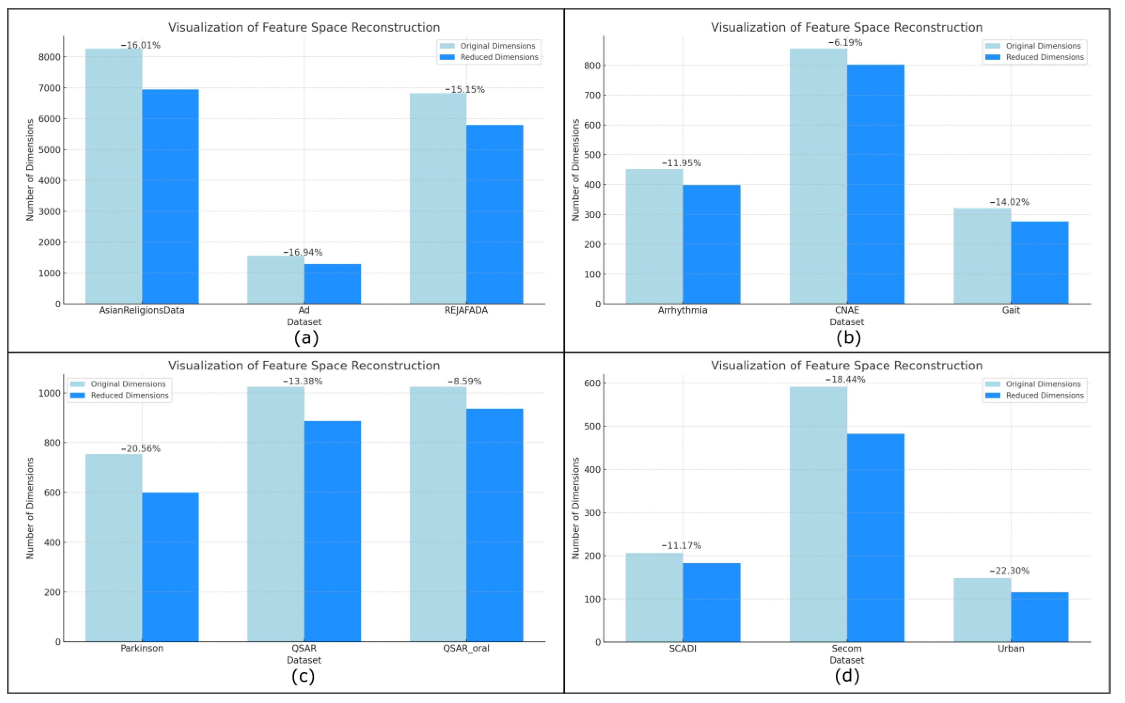
We observe that for most datasets, the reconstruction of the weak feature space using different attribute screening factors primarily impacts the classifier’s performance. Therefore, we conduct ablation experiments to explore the effectiveness of high-dimensional feature space techniques in classification tasks.

(1)

Ablation experiments based on feature space reconstruction scale

We have conducted ablation experiments to explore the contribution of the feature space reconstruction scale to the model performance. Figure 4 shows the performance of the 12 UCI high-dimensional datasets under the initial classifier ensemble with the constraint of the attribute screening factor $\beta$, demonstrating the effect of different attribute screening factors $\beta$ on classifier performance. (The box-shaped rectangle represents the fluctuation range of the data, and the upper and lower boundaries of the rectangle represent the third quartile and first quartile of the corresponding accuracy, respectively. The solid red line represents the median of the accuracy of each classifier in the classifier ensemble sorted in order, and the blue dashed line represents the accuracy mean.) Figure 5 shows the visualization of the variation of the reconstructed features.

Under the constraint of the attribute screening factor $\beta$, some of the features are optimized to be able to improve the model training accuracy to a certain extent; for example, for the AsianReligionsData dataset, the highest accuracy is only 0.8898 when the initial classifier set is trained using the original feature space in Table 2. In contrast, when β is taken to the value of 0.5, discriminative optimization is performed to the feature space, and the highest accuracy is up to 0.9062.

The possible reason for this is that optimizing some of the noisy, weakly discriminative features is information unrelated to the current classification task, and when there are strong interrelationships or repetitive information between the features, there will be multiple covariance problems, and at this time, optimizing the features will eliminate the covariance and reduce the bias in estimating the importance indices between the features. Secondly, optimizing some features can reduce the degrees of freedom, shrink the model complexity, and reduce the risk of overfitting.

Parts of the dataset for the box accuracy are more concentrated, for example, Ad, QSAR, QSAR_oral, and Secom dataset. Take the Ad dataset as an example, its $\beta =0.1$, and the accuracy of the six classifiers is as low as 0.9228, the highest is 0.9750, the fluctuation is small, but part of the dataset appeared to deviate from the data distribution of the “outlier accuracy”. For example, when Adaboost is trained on the SCADI dataset, the highest accuracy is only 0.2555 when a different $\beta$ is used to optimize the features, whereas the accuracy of other classifiers can reach 0.8860, which may be because some of the classifiers’ structures and preferences are unable to obtain the detailed feature information that is most useful for the current task, and they are unable to deal with the high-dimensional data, which will affect the classifiers’ performance. Therefore, we conduct ablation experiments to explore the effectiveness of high-dimensional feature space techniques in classification tasks.

(2)

Ablation experiment based on the classifier ensemble scale

After obtaining the feature reconstruction space for each high-dimensional dataset, we explored the effect of the number of classifiers (2, 4, 6) on the HDELC ensemble algorithm. The initial set of classifiers was decision tree (DT), random dorest (RT), Adaboost, gradient boosted (GB), extreme tree (ET), and support vector machine (SVM).

Table 4. Optimal attribute screening factors and classifier ranking order.

Dataset	$\mathbf{The} \mathbf{Best} \mathbf{of} \mathit{\beta }$	The Order of Selection for Base Classifiers
AsianReligionsData	0.5	$ET>RF>GB>SVM>DT>Adaboost$
Arrhythmia	0.4	$RF>ET>GB>SVM>Adaboost>DT$
CNAE	0.1	$GB\ge ET>SVM>RF>DT>Adaboost$
Gait	0.3	$ET>RF>GB>SVM>Adaboost>DT$
Ad	0.4	$RF>ET>Adaboost>DT>SVM>GB$
Parkinson	0.4	$GB>ET>Adaboost>RF>DT>SVM$
QSAR	0.4	$GB>ET>Adaboost>RF>DT>SVM$
QSAR_oral	0.1	$GB\ge Adaboost>SVM>ET>RF>DT$
REJAFADA	0.4	$RF>ET>GB>DT>Adaboost>SVM$
SCADI	0.2	$SVM\ge ET>RF>GB>DT>Adaboost$
Secom	0.3	$ET>GB>RF>SVM>Adaboost>DT$
Urban	0.5	$ET>GB\ge Adaboost>RF>DT>SVM$

shows the corresponding parameter settings for the 12 UCI high-dimensional datasets under the HDELC algorithm, including the optimal attribute screening factor $\beta$ corresponding to different high-dimensional datasets and the order of selection of base classifiers for the model ensemble.

For most datasets, the larger the $\beta$ setting, the higher the classification accuracy tends to be. The possible reason is that high-dimensional-data classification problems often contain more redundant information. Moreover, optimizing some weak discriminative features will enable the classifier to better capture the relationship between input and output variables and help the model improve its generalization performance. It is further demonstrated that the attribute screening factors $\beta$ can somewhat improve the model’s robustness.

After the best attribute screening factors’ selection, the accuracy of the gradient boosting tree and limit tree is relatively high. The possible reason is that random forest and gradient boosting belong to ensemble algorithms. Both are based on decision trees, which can better handle non-linear relationships, such as the classification of high-dimensional data, and have a powerful fitting ability. In general, their performance is better than that of traditional single classifiers. Moreover, from the perspective of deviation–variance analysis, random forest mainly reduces the variance term of error, while gradient boosting can reduce both variance and deviation.

Table 5. Accuracy, Recall, Precision and F1 Score for different numbers of ensemble classifiers, where the bold values denote that the best value of the indicator under the dataset.

Dataset	Model	Accuracy	Recall	Precision	F1-Score
AsianReligionsData	HDELC-2	0.8544	0.8187	0.8299	0.8243
	HDELC-4	0.8593	0.8359	0.8168	0.8262
	HDELC-6	0.8442	0.8366	0.8078	0.8219
Arrhythmia	HDELC-2	0.7214	0.7035	0.7072	0.7053
	HDELC-4	0.7408	0.7229	0.7277	0.7253
	HDELC-6	0.7351	0.7040	0.7258	0.7147
CNAE	HDELC-2	0.8888	0.9098	0.8915	0.9006
	HDELC-4	0.9231	0.9110	0.9089	0.9099
	HDELC-6	0.9437	0.9119	0.9080	0.9099
Gait	HDELC-2	0.7000	0.6838	0.6822	0.6830
	HDELC-4	0.7000	0.7676	0.7512	0.7593
	HDELC-6	0.6000	0.6172	0.5975	0.6072
Ad	HDELC-2	0.9548	0.9602	0.9630	0.9616
	HDELC-4	0.9845	0.9653	0.9579	0.9616
	HDELC-6	0.9802	0.9728	0.9732	0.9730
Parkinson	HDELC-2	0.8945	0.8882	0.8862	0.8872
	HDELC-4	0.8941	0.8808	0.8863	0.8835
	HDELC-6	0.8872	0.8721	0.8647	0.8684
QSAR	HDELC-2	0.9004	0.8969	0.8870	0.8919
	HDELC-4	0.9152	0.9012	0.9217	0.9113
	HDELC-6	0.9041	0.8991	0.9271	0.9129
QSAR_oral	HDELC-2	0.9921	0.9908	0.9910	0.9909
	HDELC-4	0.9986	0.9961	0.9950	0.9955
	HDELC-6	0.9959	0.9934	0.9949	0.9941
REJAFADA	HDELC-2	0.9844	0.9709	0.9724	0.9716
	HDELC-4	0.9826	0.9697	0.9653	0.9675
	HDELC-6	0.9733	0.9548	0.9429	0.9488
SCADI	HDELC-2	0.7842	0.7697	0.7539	0.7617
	HDELC-4	0.7861	0.8009	0.8045	0.8027
	HDELC-6	0.7622	0.7535	0.7463	0.7499
Secom	HDELC-2	0.9488	0.9409	0.9431	0.9420
	HDELC-4	0.9593	0.9443	0.9457	0.9450
	HDELC-6	0.9531	0.9441	0.9355	0.9398
Urban	HDELC-2	0.9452	0.9432	0.9305	0.9368
	HDELC-4	0.9355	0.9490	0.9314	0.9401

shows the accuracy, recall, F1-score and precision performance for the number of ensemble classifiers. Regarding classification accuracy, most datasets have the best performance in each category when the number of integrated classifiers is four, and better performance is achieved on high-dimensional datasets. Meanwhile, the Recall, Precision, and F1-score performances of HDELC-4 on Arrhythmia, Gait, SCADI, Secom, and other datasets are also significantly improved. In summary, the effectiveness and robustness of the HDELC algorithm proposed in this paper are verified.

4.3.5. Comparison of Advanced Aggregation Techniques for High-Dimensional Data

This chapter also compares HDELC with three primary traditional integrated classifiers and three integration techniques for high-dimensional data that have performed well in the existing research.

Table 6. Accuracy of advanced aggregation techniques for high-dimensional data, where the bold values denote that the best value of the indicator under the dataset.

Dataset	HDELC	Stacking	Bagging	Boosting	BOA [34]	JMO-FSCD [35]	PCA-Decision Tree [36]
AsianReligionsData	0.8651	0.8361	0.8312	0.8367	0.8518	0.8633	0.8489
Arrhythmia	0.7397	0.7225	0.7411	0.7235	0.7361	0.7402	0.7296
CNAE	0.9444	0.9152	0.8600	0.9189	0.9102	0.9428	0.9225
Gait	0.7000	0.7000	0.7000	0.6000	0.6800	0.7000	0.6808
Ad	0.9842	0.9712	0.9534	0.9430	0.9847	0.9853	0.9823
Parkinson	0.8940	0.8921	0.8917	0.8932	0.8940	0.8944	0.8924
QSAR	0.9142	0.9108	0.9000	0.9000	0.9126	0.9132	0.9044
QSAR_oral	0.9989	0.9984	0.9802	0.9885	0.9892	0.9986	0.9989
REJAFADA	0.9844	0.9825	0.9813	0.9862	0.9837	0.9836	0.9840
SCADI	0.7857	0.7910	0.8427	0.7648	0.7829	0.7806	0.7844
Secom	0.9586	0.9562	0.9278	0.9531	0.9554	0.9546	0.9569
Urban	0.9444	0.9430	0.9301	0.9429	0.9355	0.9438	0.9381

shows the performance of different integrated classifiers for high-dimensional data. It shows that the HDELC algorithm performs well on most datasets with an accuracy improvement of about 0.14% to 3.08% compared to the traditional integrated classifiers. Compared to the three integration techniques for high-dimensional data that have performed well in existing studies, the HDELC algorithm achieves better results, with an accuracy improvement of 2.2% compared to the best solution reported in the literature [34] and a certain degree of accuracy improvement compared to the JMO-FSCD algorithm proposed in the literature [35].

Meanwhile, compared with the current state-of-the-art integrated classification models, the HDELC algorithm proposed in this study has a lower computational complexity, which means that the HDELC algorithm is relatively efficient and performant and is more effective and reliable in dealing with large-scale data.

Table 7. Comparison of computational complexity of existing algorithms.

Algorithm	Computational Complexity
BEWOA [37]	$O\left(L·N·n\right)$
LightTS [38]	$O\left(E·B·P·w\right)$
AERF [39]	$O\left(D·d·m·K·n^2\right)$
HDELC	$O\left(l·m·\log m\right)$

shows the comparison of the computational complexity of existing algorithms.

4.3.6. Significance Test

We further used several non-parametric tests to determine the significance of the performance differences between the HDELC algorithm and the different ensemble algorithms, and the adjusted $p$-values associated with the various non-parametric tests are presented in

Table 8. Adjusted $p$-values for nonparametric tests (Bonferroni-Dunn, Holm, Hochberg, and Hommel tests; HDELC is the control; bold results indicate $p>0.0500$).

Algorithm	$\mathbf{Unadjusted} \mathit{p}$	${\mathit{p}}_{\mathit{B}\mathit{o}\mathit{n}\mathit{f}}$	${\mathit{p}}_{\mathit{H}\mathit{o}\mathit{l}\mathit{m}}$	${\mathit{p}}_{\mathit{B}\mathit{o}\mathit{c}\mathit{h}}$	${\mathit{p}}_{\mathit{H}\mathit{o}\mathit{m}\mathit{m}}$
Stacking	0.0037	0.0158	0.0064	0.0064	0.0064
Bagging	0.0012	0.0069	0.0038	0.0038	0.0038
Boosting	0.0056	0.0298	0.0085	0.0085	0.0085
BOA [34]	2.3006 × 10−5	2.0887 × 10−4	5.9823 × 10−5	5.9823 × 10−5	5.9823 × 10−5
JMO-FSCD [35]	5.3924 × 10−10	2.4306 × 10−9	2.6731 × 10−9	2.6731 × 10−9	2.6731 × 10−9
PCA-Decision Tree [36]	1.4489 × 10−6	1.0351 × 10−5	1.0517 × 10−6	1.0517 × 10−6	1.0517 × 10−6

and

Table 9. Adjusted $p$-values in multiple tests (Nemenyi, Holm, Bergmann and Shaffer tests, where the bold values denote that the results are not significant, where the bold values denote that the results are not significant).

Algorithm	$\mathbf{Unadjusted} \mathit{p}$	${\mathit{p}}_{\mathit{N}\mathit{e}\mathit{m}\mathit{e}}$	${\mathit{p}}_{\mathit{H}\mathit{o}\mathit{l}\mathit{m}}$	${\mathit{p}}_{\mathit{B}\mathit{e}\mathit{r}\mathit{g}}$	${\mathit{p}}_{\mathit{S}\mathit{h}\mathit{a}\mathit{f}}$
HDELC vs. Stacking	0.0037	0.1052	0.0489	0.0396	0.0472
HDELC vs. Bagging	0.0012	0.0069	0.0038	0.0038	0.0038
HDELC vs. Boosting	0.0056	0.1398	0.0540	0.0481	0.0527
HDELC vs. BOA [34]	2.3006 × 10−5	6.4290 × 10−4	4.6833 × 10−4	3.5772 × 10−4	4.2085 × 10−4
HDELC vs. PCA-Decision Tree [35]	1.4489 × 10−6	5.7897 × 10−5	4.9836 × 10−5	2.5539 × 10−5	4.6791 × 10−5
HDELC vs. JMO-FSCD [36]	5.3924 × 10−10	1.2764 × 10−8	1.2273 × 10−8	1.0784 × 10−8	1.0784 × 10−8

.

Based on the adjusted $p$-values associated with the different nonparametric tests listed in Table 8 and Table 9, comparing each adjusted p-value with the significance threshold, most of the adjusted $p$-values are less than the significance threshold, and the corresponding comparisons can be considered as statistically significant, which further confirms the significant performance improvement and enhancement of the HDELC algorithm over other current state-of-the-art classifiers ensemble algorithms. Nonparametric tests can combine accurate, reliable statistics test references with complexity in multiple comparisons.

5. Conclusions and Future Work

In this paper, the classification problem for high-dimensional data is investigated. According to the characteristics of the dataset and the requirements of the problem, a subspace integration algorithm under high-dimensional spatial reconstruction (HDELC algorithm) is proposed, which considers the feature space and the model integration and solves the problem of the low computational efficiency of high-dimensional data in the process of model training, and can obtain a more accurate, stable, and robust final result. The feature reconstruction matrix and the HDELC algorithm cost function are designed to eliminate redundant features, obtain a more helpful feature space, and optimize the computational performance of the integrated system. In addition, ablation experiments are set up to explore the contributions of the feature selection and classifier integration components, and the sensitivity analysis of the attribute screening factors and the changes in feature space reconstruction are visualized. Comparisons are made with six state-of-the-art integration techniques targeting high-dimensional data on 12 benchmark datasets, and the experimental results show that the HDELC algorithm outperforms the comparison algorithms in terms of several metrics such as classification accuracy, recall, etc., with an improvement in precision of about 3.08% or so and a maximum accuracy of 0.9989.

In the future, we will consider constructing artificial datasets that investigate ensemble models for dealing with noise intensity, extreme outliers, and inhomogeneous distributions of data points of predictor variables, alongside exploring the advantages of integrated learning in data analysis and processing.

References

1. Sharma, A.; Kaur, A.; Singh, K.; Upadhyay, S.K. Modulation in gene expression and enzyme activity suggested the roles of monodehydroascorbate reductase in development and stress response in bread wheat. Plant Sci. 2024, 338, 111902. [Google Scholar]
2. Ansori, M.A.Z.; Solehudin, E. Analysis of the Syar’u Man Qablana Theory and its Application in Sharia Financial Institutions. Al-Afkar J. Islam. Stud. 2024, 7, 590–607. [Google Scholar]
3. Tartarisco, G.; Cicceri, G.; Bruschetta, R.; Tonacci, A.; Campisi, S.; Vitabile, S.; Cerasa, A.; Distefano, S.; Pellegrino, A.; Modesti, P.A. An intelligent Medical Cyber–Physical System to support heart valve disease screening and diagnosis. Expert Syst. Appl. 2024, 238, 121772. [Google Scholar] [CrossRef]
4. Liu, L. Analyst monitoring and information asymmetry reduction: US evidence on environmental investment. Innov. Green Dev. 2024, 3, 100098. [Google Scholar] [CrossRef]
5. Lee, K.; Laskin, M.; Srinivas, A.; Abbeel, P. Sunrise: A simple unified framework for ensemble learning in deep reinforcement learning. In Proceedings of the International Conference on Machine Learning, Online, 18–24 July 2021; pp. 6131–6141. [Google Scholar]
6. Campagner, A.; Ciucci, D.; Cabitza, F. Aggregation models in ensemble learning: A large-scale comparison. Inf. Fusion 2023, 90, 241–252. [Google Scholar] [CrossRef]
7. Zhu, X.; Li, J.; Ren, J.; Wang, J.; Wang, G. Dynamic ensemble learning for multi-label classification. Inf. Sci. 2023, 623, 94–111. [Google Scholar] [CrossRef]
8. Asadi, B.; Hajj, R. Prediction of asphalt binder elastic recovery using tree-based ensemble bagging and boosting models. Constr. Build. Mater. 2024, 410, 134154. [Google Scholar] [CrossRef]
9. Sun, Z.; Wang, G.; Li, P.; Wang, H.; Zhang, M.; Liang, X. An improved random forest based on the classification accuracy and correlation measurement of decision trees. Expert Syst. Appl. 2024, 237, 121549. [Google Scholar] [CrossRef]
10. Jiang, J.; Liu, F.; Ng, W.W.; Tang, Q.; Wang, W.; Pham, Q.V. Dynamic incremental ensemble fuzzy classifier for data streams in green internet of things. IEEE Trans. Green Commun. Netw. 2022, 6, 1316–1329. [Google Scholar] [CrossRef]
11. Lughofer, E.; Pratama, M. Evolving multi-user fuzzy classifier system with advanced explainability and interpretability aspects. Inf. Fusion 2023, 91, 458–476. [Google Scholar] [CrossRef]
12. Pérez, E.; Ventura, S. An ensemble-based convolutional neural network model powered by a genetic algorithm for melanoma diagnosis. Neural Comput. Appl. 2022, 34, 10429–10448. [Google Scholar] [CrossRef]
13. Deb, S.D.; Jha, R.K.; Jha, K.; Tripathi, P.S. A multi model ensemble based deep convolution neural network structure for detection of COVID-19. Biomed. Signal Process. Control. 2022, 71, 103126. [Google Scholar] [CrossRef]
14. Liu, B.; Li, X.; Xiao, Y.; Sun, P.; Zhao, S.; Peng, T.; Zheng, Z.; Huang, Y. Adaboost-based SVDD for anomaly detection with dictionary learning. Expert Syst. Appl. 2024, 238, 121770. [Google Scholar] [CrossRef]
15. Kedia, V.; Chakraborty, D. Randomized Subspace Identification for LTI Systems. In Proceedings of the 2023 European Control Conference (ECC), Bucharest, Romania, 13–16 June 2023; IEEE: Piscataway, NJ, USA, 2023; pp. 1–6. [Google Scholar]
16. Hart, J.L.; Bhatt, L.; Zhu, Y.; Han, M.G.; Bianco, E.; Li, S.; Hynek, D.J.; Schneeloch, J.A.; Tao, Y.; Louca, D. Emergent layer stacking arrangements in c-axis confined MoTe2. Nat. Commun. 2023, 14, 4803. [Google Scholar] [CrossRef]
17. Li, X.; Wang, Y.; Tang, B.; Qin, Y.; Zhang, G. Canonical correlation analysis of dimension reduced degradation feature space for machinery condition monitoring. Mech. Syst. Signal Process. 2023, 182, 109603. [Google Scholar] [CrossRef]
18. Priyadarshini, J.; Premalatha, M.; Čep, R.; Jayasudha, M.; Kalita, K. Analyzing physics-inspired metaheuristic algorithms in feature selection with K-nearest-neighbor. Appl. Sci. 2023, 13, 906. [Google Scholar] [CrossRef]
19. Li, Y.; Chai, Y.; Zhou, H.; Yin, H. A novel dimension reduction and dictionary learning framework for high-dimensional data classification. Pattern Recognit. 2021, 112, 107793. [Google Scholar] [CrossRef]
20. Wang, Q.; Nguyen, T.T.; Huang, J.Z.; Nguyen, T.T. An efficient random forests algorithm for high dimensional data classification. Adv. Data Anal. Classif. 2018, 12, 953–972. [Google Scholar] [CrossRef]
21. Uddin, K.M.M.; Biswas, N.; Rikta, S.T.; Dey, S.K. Machine learning-based diagnosis of breast cancer utilizing feature optimization technique. Comput. Methods Programs Biomed. Update 2023, 3, 100098. [Google Scholar] [CrossRef]
22. Tékouabou, S.C.K.; Chabbar, I.; Toulni, H.; Cherif, W.; Silkan, H. Optimizing the early glaucoma detection from visual fields by combining preprocessing techniques and ensemble classifier with selection strategies. Expert Syst. Appl. 2022, 189, 115975. [Google Scholar] [CrossRef]
23. Xu, C.; Zhang, S. A Genetic Algorithm-based sequential instance selection framework for ensemble learning. Expert Syst. Appl. 2024, 236, 121269. [Google Scholar] [CrossRef]
24. Kurutach, T.; Clavera, I.; Duan, Y.; Tamar, A.; Abbeel, P. Model-ensemble trust-region policy optimization. arXiv 2018, arXiv:1802.10592. [Google Scholar]
25. Ahmed, K.; Sachindra, D.A.; Shahid, S.; Iqbal, Z.; Nawaz, N.; Khan, N. Multi-model ensemble predictions of precipitation and temperature using machine learning algorithms. Atmos. Res. 2020, 236, 104806. [Google Scholar] [CrossRef]
26. Zhong, Y.; Chen, W.; Wang, Z.; Chen, Y.; Wang, K.; Li, Y.; Yin, X.; Shi, X.; Yang, J.; Li, K. HELAD: A novel network anomaly detection model based on heterogeneous ensemble learning. Comput. Netw. 2020, 169, 107049. [Google Scholar] [CrossRef]
27. Rudy, S.H.; Sapsis, T.P. Output-weighted and relative entropy loss functions for deep learning precursors of extreme events. Phys. D Nonlinear Phenom. 2023, 443, 133570. [Google Scholar] [CrossRef]
28. Wu, K.; Chen, P.; Ghattas, O. A Fast and Scalable Computational Framework for Large-Scale High-Dimensional Bayesian Optimal Experimental Design. SIAM/ASA J. Uncertain. Quantif. 2023, 11, 235–261. [Google Scholar] [CrossRef]
29. Chen, J.; Xu, A.; Chen, D.; Zhang, Y.; Chen, Z. Discrete Boltzmann modeling of Rayleigh-Taylor instability: Effects of interfacial tension, viscosity, and heat conductivity. Phys. Rev. E 2022, 106, 015102. [Google Scholar] [CrossRef]
30. Shin, M.; Lee, J.; Jeong, K. Estimating quantum mutual information through a quantum neural network. Quantum Inf. Process. 2024, 23, 57. [Google Scholar] [CrossRef]
31. Du, L.; Liu, H.; Zhang, L.; Lu, Y.; Li, M.; Hu, Y.; Zhang, Y. Deep ensemble learning for accurate retinal vessel segmentation. Comput. Biol. Med. 2023, 158, 106829. [Google Scholar] [CrossRef]
32. Lv, Y.; Lu, J.; Liu, Y.; Zhang, L. A class of stealthy attacks on remote state estimation with intermittent observation. Inf. Sci. 2023, 639, 118964. [Google Scholar] [CrossRef]
33. Dua, D.; Graff, C. UCI Machine Learning Repository; University of California, School of Information and Computer Science: Irvine, CA, USA, 2019; Available online: http://archive.ics.uci.edu/ml (accessed on 1 February 2023).
34. Elminaam, D.S.A.; Nabil, A.; Ibraheem, S.A.; Houssein, E.H. An Efficient Marine Predators Algorithm for Feature Selection. IEEE Access 2021, 9, 60136–60153. [Google Scholar] [CrossRef]
35. Bai, L.; Li, H.; Gao, W.; Xie, J.; Wang, H. A joint multiobjective optimization of feature selection and classifier design for high-dimensional data classification. Inf. Sci. 2023, 626, 457–473. [Google Scholar] [CrossRef]
36. Ibrahim, S.; Nazir, S.; Velastin, S.A. Feature selection using correlation analysis and principal component analysis for accurate breast cancer diagnosis. J. Imaging 2021, 7, 225. [Google Scholar] [CrossRef]
37. Mafarja, M.; Thaher, T.; Al-Betar, M.A.; Too, J.; Awadallah, M.A.; Abu Doush, I.; Turabieh, H. Classification framework for faulty-software using enhanced exploratory whale optimizer-based feature selection scheme and random forest ensemble learning. Appl. Intell. 2023, 53, 18715–18757. [Google Scholar] [CrossRef] [PubMed]
38. Campos, D.; Zhang, M.; Yang, B.; Kieu, T.; Guo, C.; Jensen, C.S. LightTS: Lightweight Time Series Classification with Adaptive Ensemble Distillation. Proc. ACM Manag. Data 2023, 1, 1–27. [Google Scholar] [CrossRef]
39. Jiang, J.; Liu, F.; Ng, W.W.; Tang, Q.; Zhong, G.; Tang, X.; Wang, B. AERF: Adaptive ensemble random fuzzy algorithm for anomaly detection in cloud computing. Comput. Commun. 2023, 200, 86–94. [Google Scholar] [CrossRef]
Figure 1. Structure of the HDELC approach.
Applsci 14 01956 g001
Figure 2. Illustration of the process of feature space selection and reconstruction.
Applsci 14 01956 g002
Figure 3. Attribute screening factor sensitivity analysis visualization results (partial). (a) AsianReligionsData dataset. (b) Arrhythmia dataset. (c) Ad dataset. (d) QSAR dataset.
Applsci 14 01956 g003
Figure 4. Influence of attribute exclusion factor β on classifier performance, where “*” represents an outlier point, the solid red line represents the median of the accuracy of each classifier in the classifier ensemble sorted in order, and the blue dashed line represents the accuracy mean.
Applsci 14 01956 g004
Figure 5. Visualization results of changes in feature space after reconstruction. (a) AsianReligionsData, Ad and REJAFADA dataset. (b) Arrhythmia, CNAE and Gait dataset. (c) Parkinson QSAR and QSAR_oral dataset. (d) SCADI, Secom and Urban dataset.
Applsci 14 01956 g005