
Optimization of Redundant Degrees of Freedom in Robotic Flat-End Milling Based on Dynamic Response

Abstract
1. Introduction
2. Redundant Degrees of Freedom Optimization in Robotic Milling
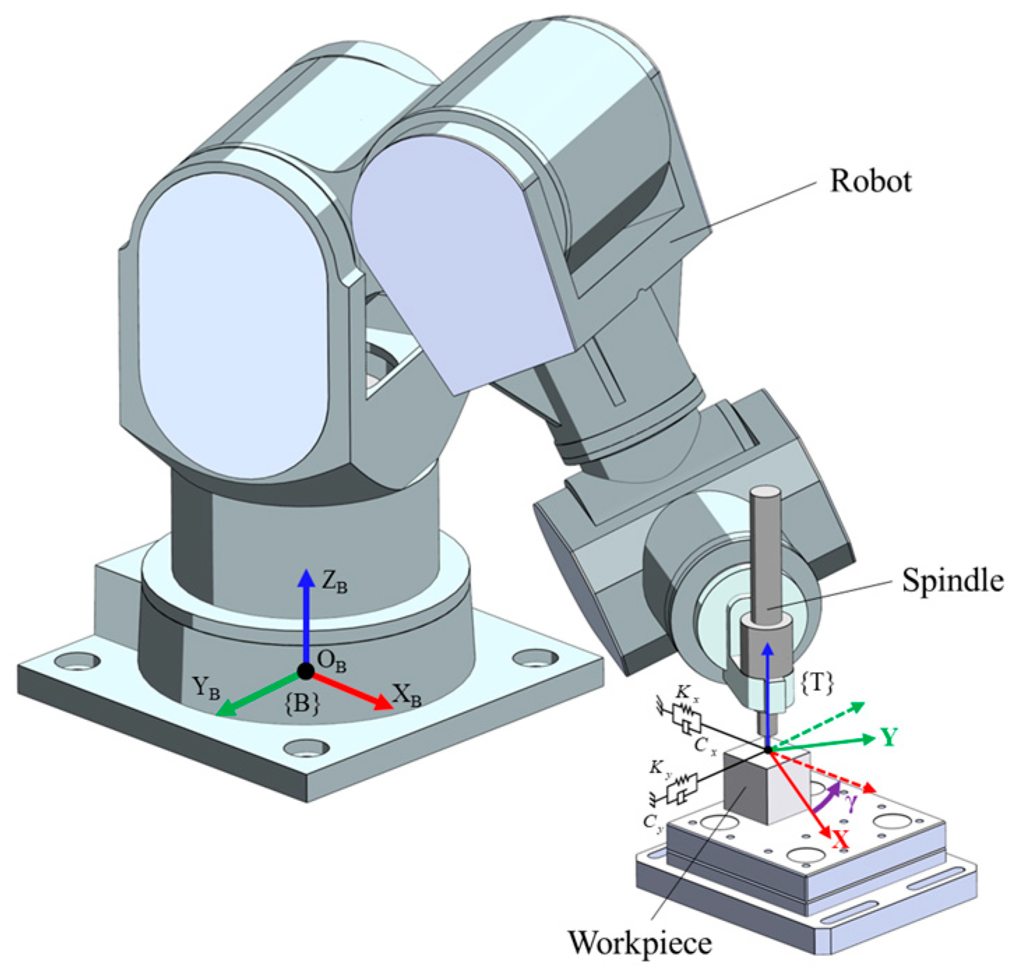
2.1. Problem Description of Redundant Degrees of Freedom in Robotic Milling
2.2. Redundant Degree of Freedom Optimization Model Considering Tool Vibration
2.3. Solution of Redundant Degree of Freedom Optimization Model
2.3.1. Evaluation of Posture-Dependent Frequency Response Function
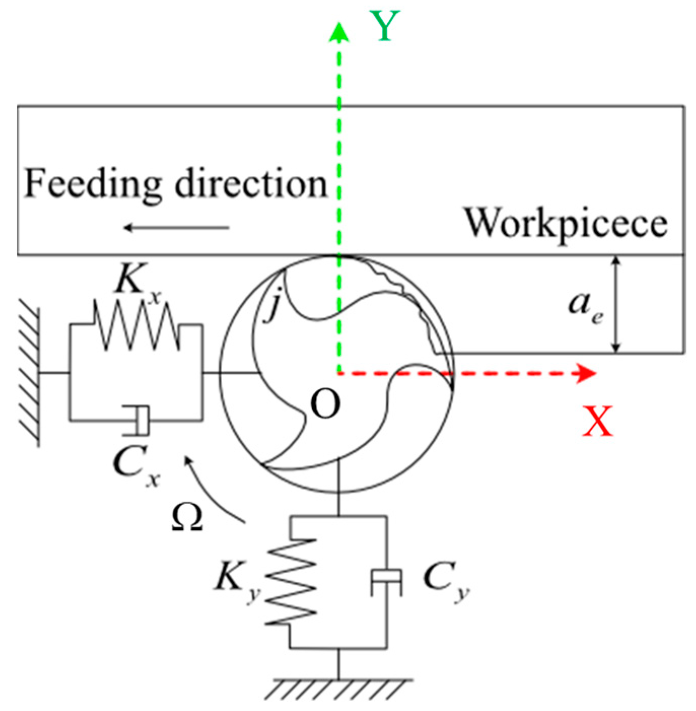
2.3.2. Dynamic Model of a Robotic Milling System
2.3.3. Regenerative Chatter Analysis of a Robotic Milling System
2.3.4. Dynamic Response Index in Robotic Milling
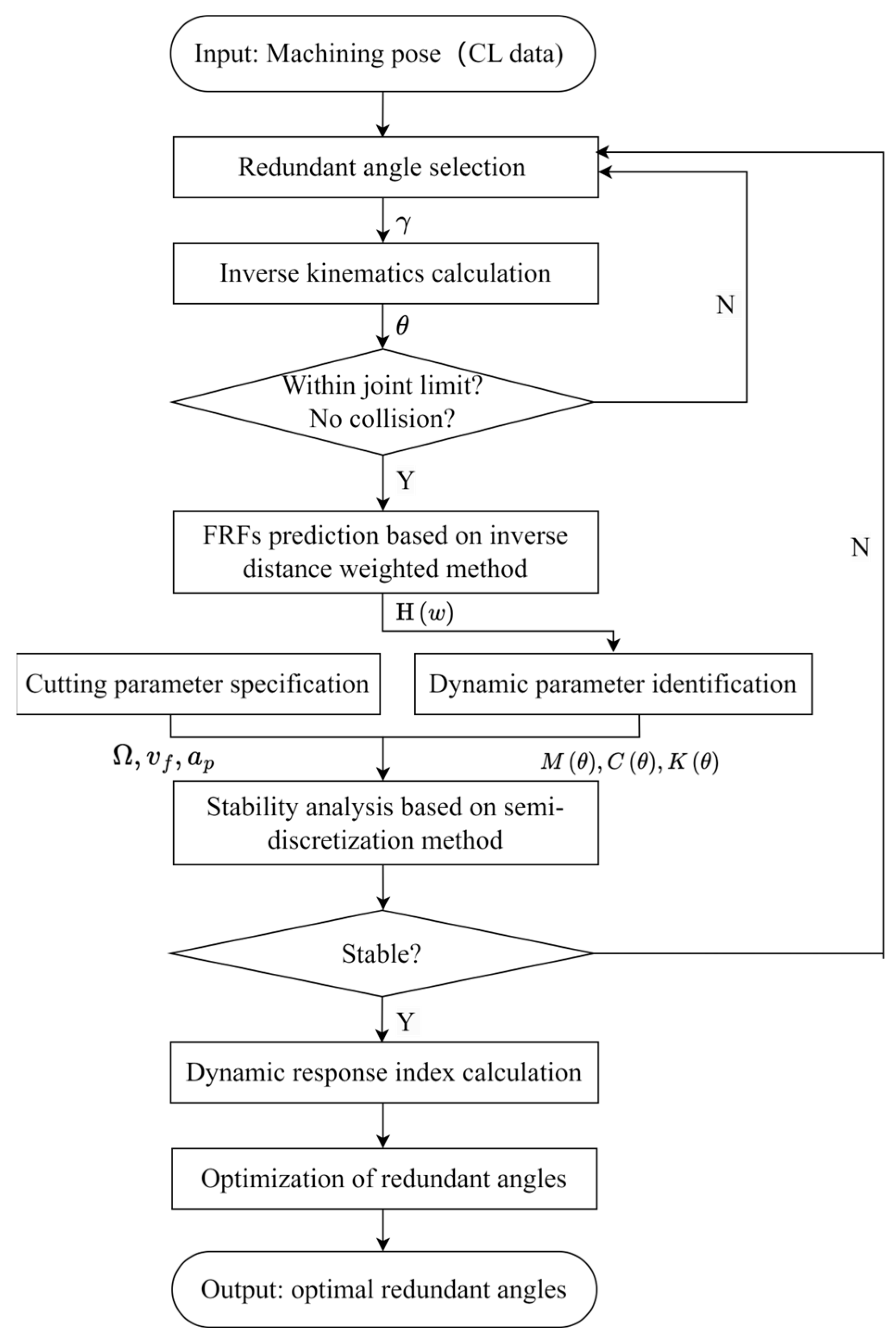
2.4. Flowchart for Solving the Redundant Degree of Freedom Optimization Model
3. Milling Experimental Validation
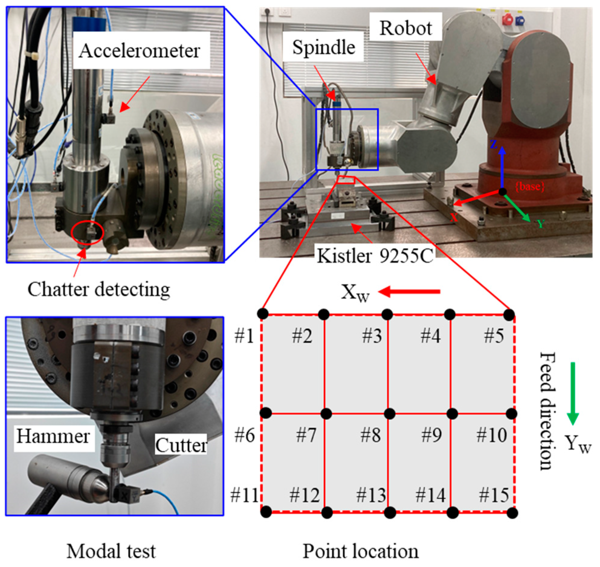
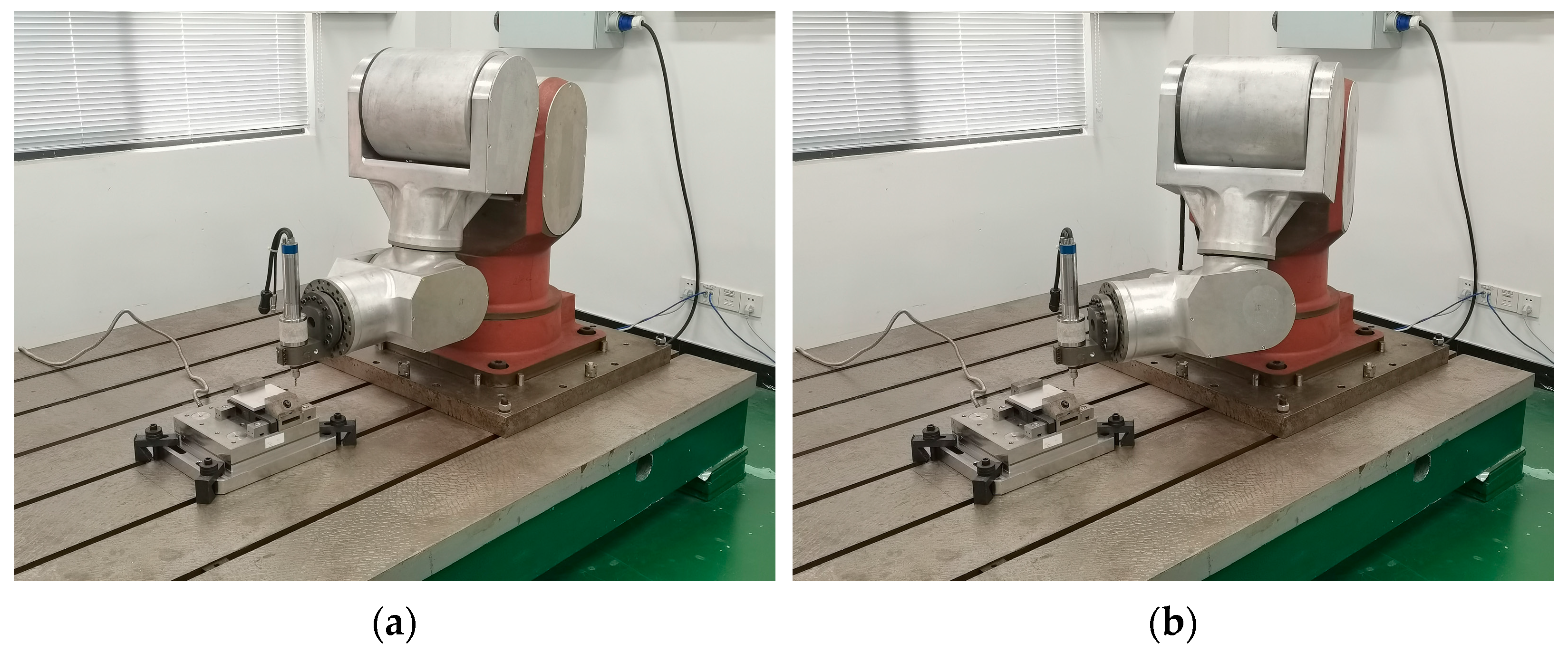
3.1. Experimental Setup
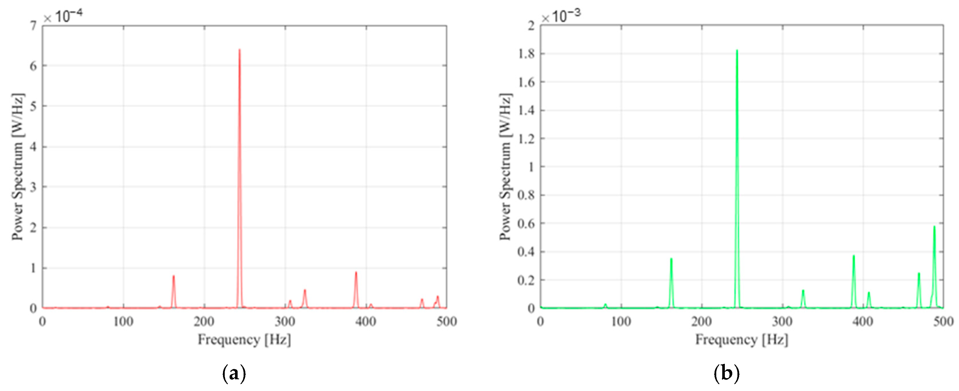
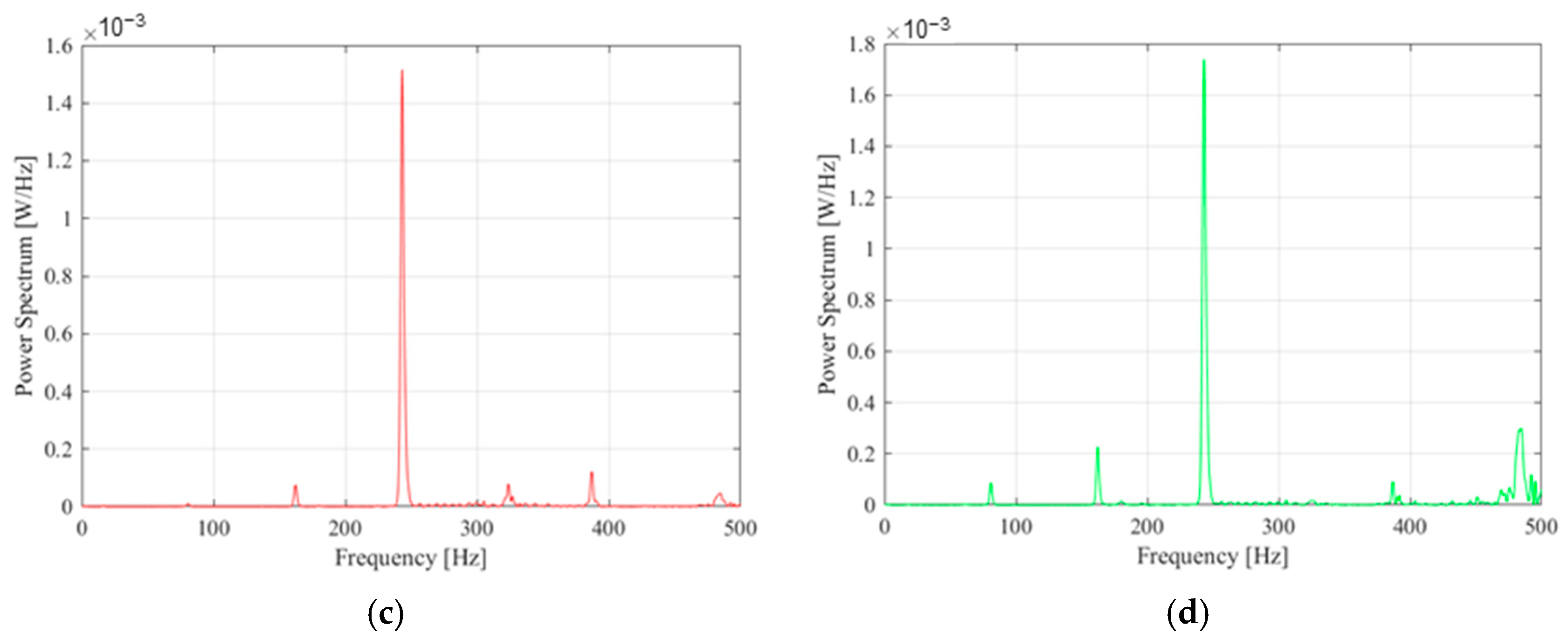
3.2. Modal Parameter Identification
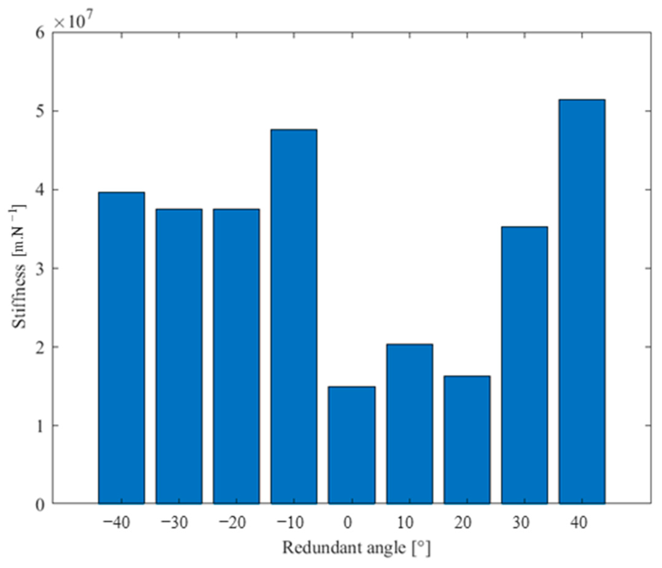
3.3. Analysis of Milling Stability with Redundant Angles
3.4. Posture Optimization Based on the Dynamic Response Index
4. Conclusions
Author Contributions
Funding
Data Availability Statement
Conflicts of Interest
Nomenclatures
| The unit vector representing the direction of the tool axis | |
| X–Y–Z Euler angle | |
| Homogeneous transformation matrix of the tool coordinate system relative to the workpiece coordinate system | |
| The l-th element in the peak vector of the vibration signal | |
| The total number of elements in the peak vector | |
| The vibration displacement in the specified direction, with superscript p denoting the point P, and subscript l indicating the l-th element | |
| Inverse kinematics | |
| Joint angle | |
| The state transfer matrix | |
| The number of the tested postures | |
| , | The frequency response function of posture ,, respectively |
| The Euclidean distance in joint space | |
| The predicted frequency response function at the nodes g and h. | |
| Frequency in rad/s | |
| The number of modes | |
| i | The imaginary unit |
| The residues at nodes g and h of mode r | |
| A modal scaling constant | |
| ,, | The pole, damping ratio, natural frequency of mode r |
| The mode shape coefficients in nodes g and h for mode r | |
| M(θ), C(θ) and K(θ) | The posture-dependent modal mass, damping, and stiffness matrix |
| The modal mass, damping and stiffness matrices of the system along the x and y directions | |
| Cutting force | |
| Cutting depth | |
| The specific directional coefficients matrix | |
| A unit step function | |
| Cutting width | |
| , | The tangential force coefficient and radial force coefficient |
| The angular position of j-th tooth | |
| Number of teeth | |
| Spindle speed in r/min | |
| Cutting force vector | |
| Feed per tooth | |
| Time periodic matrix | |
| Delay time | |
| The identity matrix | |
| The initial state matrix | |
| Feeding velocity |
Appendix A

| Posture | Joint Angle (°) | Posture | Joint Angle (°) | ||
|---|---|---|---|---|---|
| −40° | #2 | 25.22, 9.89, 29.42, 70.34, 74.60, −36.63 | 10° | #2 | −10.15, 24.05, −1.38, −21.69, 68.79, 8.19 |
| #6 | 23.76, 4.62, 39.66, 70.57, 72.02, −41.18 | #6 | −9.38, 21.09, 5.71, −21.51, 64.83, 9.52 | ||
| #10 | 29.70, −2.21, 52.36, 76.67, 74.55, −48.34 | #10 | −0.65, 21.65, 4.40, −11.82, 64.43, 5.16 | ||
| #14 | 27.52, −4.10, 55.79, 75.61, 72.54, −49.47 | #14 | −2.75, 19.96, 8.29, −14.40, 62.51, 6.76 | ||
| −30° | #2 | 21.42, 17.16, 14.45, 55.81, 70.92, −25.69 | 20° | #2 | −17.71, 21.29, 5.24, −40.83, 69.30, 16.98 |
| #6 | 20.04, 13.23, 22.69, 55.84, 67.86, −29.05 | #6 | −16.47, 17.97, 12.68, −40.67, 65.78.19.41 | ||
| #10 | 26.78, 9.31, 30.57, 63.32, 69.44, −34.96 | #10 | −8.38, 19.53, 9.24, −31.64, 64.94, 14.63 | ||
| #14 | 24.41, 8.03, 33.09, 61.67, 67.50, −35.37 | #14 | −10.08, 17.43, 13.85, −34.13, 63.29, 16.94 | ||
| −20° | #2 | 15.60, 21.75, 4.18, 38.53, 69.18, −15.80 | 30° | #2 | −23.26, 16.41, 16.05, −57.80, 71.27, 27.02 |
| #6 | 14.50, 18.47, 11.61, 38.45, 65.61, −18.16 | #6 | −21.79, 12.41, 24.38, −57.77, 68.26, 30.43 | ||
| #10 | 26.78, 9.31, 30.57, 63.32, 69.44, −34.96 | #10 | −14.56, 15.19, 18.64, −49.85, 66.63, 25.19 | ||
| #14 | 19.63, 14.83, 19.38, 45.04, 64.34, −23.44 | #14 | −15.90, 12.46, 24.27, −52.16, 65.41, 28.19 | ||
| −10° | #2 | 7.82, 24.26, −1.91, 19.17, 68.78, −7.17 | 40° | #2 | −26.83, 8.72, 31.73, −71.96, 75.21, 38.09 |
| #6 | 7.23, 21.33, 5.17, 19.11, 64.78, −8.40 | #6 | −25.31, 3.23, 42.30, −72.14, 72.66, 42.78 | ||
| #10 | 15.68, 20.01, 8.18, 28.62, 64.80, −13.08 | #10 | −18.92, 7.92, 33.30, −65.61, 70.11, 36.88 | ||
| #14 | 13.13, 18.74, 11.01, 26.20, 62.85, −12.65 | #14 | −19.98, 4.01, 40.81, −67.71, 69.35, 40.71 | ||
| 0° | #2 | −1.21, 25.00, −3.78, −1.30, 68.79, 0.47 | |||
| #6 | −1.12, 22.17, 3.20, −1.24, 64.64, 0.53 | ||||
| #10 | 7.77, 21.80, 4.05, 8.62, 64.40, −3.75 | ||||
| #14 | 5.36, 20.38, 7.34, 6.05, 62.41, −2.81 | ||||
References
- Wang, W.; Guo, Q.; Yang, Z.; Jiang, Y.; Xu, J. A State-of-the-Art Review on Robotic Milling of Complex Parts with High Efficiency and Precision. Robot. Comput.-Integr. Manuf. 2023, 79, 102436. [Google Scholar] [CrossRef]
- Yuan, H.; Courteille, E.; Deblaise, D. Static and Dynamic Stiffness Analyses of Cable-Driven Parallel Robots with Non-Negligible Cable Mass and Elasticity. Mech. Mach. Theory 2015, 85, 64–81. [Google Scholar] [CrossRef]
- Zhu, Z.; Tang, X.; Chen, C.; Peng, F.; Yan, R.; Zhou, L.; Li, Z.; Wu, J. High Precision and Efficiency Robotic Milling of Complex Parts: Challenges, Approaches and Trends. Chin. J. Aeronaut. 2022, 35, 22–46. [Google Scholar] [CrossRef]
- Bu, Y.; Liao, W.; Tian, W.; Zhang, J.; Zhang, L. Stiffness Analysis and Optimization in Robotic Drilling Application. Precis. Eng. 2017, 49, 388–400. [Google Scholar] [CrossRef]
- Li, G.; Zhu, W.; Dong, H.; Ke, Y. Stiffness-Oriented Performance Indices Defined on Two-Dimensional Manifold for 6-DOF Industrial Robot. Robot. Comput.-Integr. Manuf. 2021, 68, 102076. [Google Scholar] [CrossRef]
- Slavkovic, N.R.; Milutinovic, D.S.; Glavonjic, M.M. A Method for Off-Line Compensation of Cutting Force-Induced Errors in Robotic Machining by Tool Path Modification. Int. J. Adv. Manuf. Technol. 2014, 70, 2083–2096. [Google Scholar] [CrossRef]
- Liu, C.; Li, Y.; Shen, W. A Real Time Machining Error Compensation Method Based on Dynamic Features for Cutting Force Induced Elastic Deformation in Flank Milling. Mach. Sci. Technol. 2018, 22, 766–786. [Google Scholar] [CrossRef]
- Jin, Y.; Gu, Q.; Liu, S.; Yang, C. Experimental Investigation and Modeling of Force-Induced Surface Errors for the Robot-Assisted Milling Process. Machines 2023, 11, 655. [Google Scholar] [CrossRef]
- Mohammadi, Y.; Ahmadi, K. Chatter in Milling with Robots with Structural Nonlinearity. Mech. Syst. Signal Process. 2021, 167, 108523. [Google Scholar] [CrossRef]
- Gao, K.; Zhou, X.; Wang, R.; Fan, M.; Han, H. Robotic Milling Stability Optimization Based on Robot Functional Redundancy. Ind. Robot Int. J. Robot. Res. Appl. 2023, 50, 1036–1047. [Google Scholar] [CrossRef]
- Huo, L.; Baron, L. The Self-Adaptation of Weights for Joint-Limits and Singularity Avoidances of Functionally Redundant Robotic-Task. Robot. Comput.-Integr. Manuf. 2011, 27, 367–376. [Google Scholar] [CrossRef]
- Xiao, W.; Strauß, H.; Loohß, T.; Hoffmeister, H.-W.; Hesselbach, J. Closed-Form Inverse Kinematics of 6R Milling Robot with Singularity Avoidance. Prod. Eng. Res. Devel. 2011, 5, 103–110. [Google Scholar] [CrossRef]
- Xiao, W.; Huan, J. Redundancy and Optimization of a 6R Robot for Five-Axis Milling Applications: Singularity, Joint Limits and Collision. Prod. Eng. Res. Devel. 2012, 6, 287–296. [Google Scholar] [CrossRef]
- Shi, Z.; Zhang, W.; Ding, Y. A Local Toolpath Smoothing Method for a Five-Axis Hybrid Machining Robot. Sci. China Technol. Sci. 2023, 66, 721–742. [Google Scholar] [CrossRef]
- Zhang, Y.; Li, S.; Kadry, S.; Liao, B. Recurrent Neural Network for Kinematic Control of Redundant Manipulators With Periodic Input Disturbance and Physical Constraints. IEEE Trans. Cybern. 2019, 49, 4194–4205. [Google Scholar] [CrossRef] [PubMed]
- Mitsi, S.; Bouzakis, K.-D.; Sagris, D.; Mansour, G. Determination of Optimum Robot Base Location Considering Discrete End-Effector Positions by Means of Hybrid Genetic Algorithm. Robot. Comput.-Integr. Manuf. 2008, 24, 50–59. [Google Scholar] [CrossRef]
- Zeng, Y.; Tian, W.; Liao, W. Positional Error Similarity Analysis for Error Compensation of Industrial Robots. Robot. Comput.-Integr. Manuf. 2016, 42, 113–120. [Google Scholar] [CrossRef]
- Xiong, G.; Li, Z.; Ding, Y.; Zhu, L. A Closed-Loop Error Compensation Method for Robotic Flank Milling. Robot. Comput.-Integr. Manuf. 2020, 63, 101928. [Google Scholar] [CrossRef]
- Xie, F.; Chen, L.; Li, Z.; Tang, K. Path Smoothing and Feed Rate Planning for Robotic Curved Layer Additive Manufacturing. Robot. Comput.-Integr. Manuf. 2020, 65, 101967. [Google Scholar] [CrossRef]
- Lin, Y.; Zhao, H.; Ding, H. Posture Optimization Methodology of 6R Industrial Robots for Machining Using Performance Evaluation Indexes. Robot. Comput.-Integr. Manuf. 2017, 48, 59–72. [Google Scholar] [CrossRef]
- Kelaiaia, R. Improving the Pose Accuracy of the Delta Robot in Machining Operations. Int. J. Adv. Manuf. Technol. 2017, 91, 2205–2215. [Google Scholar] [CrossRef]
- Peng, J.; Ding, Y.; Zhang, G.; Ding, H. Smoothness-Oriented Path Optimization for Robotic Milling Processes. Sci. China Technol. Sci. 2020, 63, 1751–1763. [Google Scholar] [CrossRef]
- Chen, C.; Peng, F.; Yan, R.; Li, Y.; Wei, D.; Fan, Z.; Tang, X.; Zhu, Z. Stiffness Performance Index Based Posture and Feed Orientation Optimization in Robotic Milling Process. Robot. Comput.-Integr. Manuf. 2019, 55, 29–40. [Google Scholar] [CrossRef]
- Garnier, S.; Dumas, C.; Caro, S.; Furet, B. Quality Certification and Productivity Optimization in Robotic-Based Manufacturing. IFAC Proc. Vol. 2013, 46, 825–830. [Google Scholar] [CrossRef]
- Liao, Z.; Li, J.; Xie, H.; Wang, Q.; Zhou, X. Region-Based Toolpath Generation for Robotic Milling of Freeform Surfaces with Stiffness Optimization. Robot. Comput.-Integr. Manuf. 2020, 64, 101953. [Google Scholar] [CrossRef]
- Chen, Q.; Zhang, C.; Hu, T.; Zhou, Y.; Ni, H.; Xue, X. Posture Optimization in Robotic Machining Based on Comprehensive Deformation Index Considering Spindle Weight and Cutting Force. Robot. Comput.-Integr. Manuf. 2022, 74, 102290. [Google Scholar] [CrossRef]
- Lee, J.H.; Kim, S.H.; Min, B.-K. Posture Optimization in Robotic Drilling Using a Deformation Energy Model. Robot. Comput.-Integr. Manuf. 2022, 78, 102395. [Google Scholar] [CrossRef]
- Celikag, H.; Sims, N.D.; Ozturk, E. Chatter Suppression in Robotic Milling by Control of Configuration Dependent Dynamics. Procedia CIRP 2019, 82, 521–526. [Google Scholar] [CrossRef]
- Mohammed, A.; Schmidt, B.; Wang, L. Energy-Efficient Robot Configuration for Assembly. J. Manuf. Sci. Eng. 2017, 139, 051007. [Google Scholar] [CrossRef]
- Mousavi, S.; Gagnol, V.; Bouzgarrou, B.C.; Ray, P. Stability Optimization in Robotic Milling through the Control of Functional Redundancies. Robot. Comput.-Integr. Manuf. 2018, 50, 181–192. [Google Scholar] [CrossRef]
- Xiong, X.; Li, Y.; Qin, H. Structural Dynamic Performance Evaluation of Industrial Robots Based on Vibration Tests. In Proceedings of the 2018 IEEE 4th Information Technology Mechatronics Eng Conference, Chongqing, China, 14–16 December 2018; pp. 302–306. [Google Scholar] [CrossRef]
- Cvitanic, T.; Nguyen, V.; Melkote, S.N. Pose Optimization in Robotic Machining Using Static and Dynamic Stiffness Models. Robot. Comput.-Integr. Manuf. 2020, 66, 101992. [Google Scholar] [CrossRef]
- Wang, L.; Liu, Y.; Yu, Y.; Zhang, J.; Shu, B. Optimization of Redundant Degree of Freedom in Robotic Milling Considering Chatter Stability. Int. J. Adv. Manuf. Technol. 2022, 121, 8379–8394. [Google Scholar] [CrossRef]
- Hou, T.; Lei, Y.; Ding, Y. Pose Optimization in Robotic Milling Based on Surface Location Error. J. Manuf. Sci. Eng. 2023, 145, 084501. [Google Scholar] [CrossRef]
- Aenlle, M.; Juul, M.; Brincker, R. Modal Mass and Length of Mode Shapes in Structural Dynamics. Shock Vib. 2020, 2020, 8648769. [Google Scholar] [CrossRef]
- Brandt, A.; Berardengo, M.; Manzoni, S.; Cigada, A. Scaling of Mode Shapes from Operational Modal Analysis Using Harmonic Forces. J. Sound Vib. 2017, 407, 128–143. [Google Scholar] [CrossRef]
- Chen, C.; Peng, F.; Yan, R.; Fan, Z.; Li, Y.; Wei, D. Posture-Dependent Stability Prediction of a Milling Industrial Robot Based on Inverse Distance Weighted Method. Procedia Manuf. 2018, 17, 993–1000. [Google Scholar] [CrossRef]
- Chen, C.; Peng, F.; Yan, R.; Tang, X.; Li, Y.; Fan, Z. Rapid Prediction of Posture-Dependent FRF of the Tool Tip in Robotic Milling. Robot. Comput.-Integr. Manuf. 2020, 64, 101906. [Google Scholar] [CrossRef]
- Lei, Y.; Hou, T.; Ding, Y. Prediction of the Posture-Dependent Tool Tip Dynamics in Robotic Milling Based on Multi-Task Gaussian Process Regressions. Robot. Comput.-Integr. Manuf. 2023, 81, 102508. [Google Scholar] [CrossRef]
- Altintas, Y. Manufacturing Automation: Metal Cutting Mechanics, Machine Tool Vibrations, and CNC Design, 2nd ed.; Cambridge University Press: Cambridge, UK, 2012; ISBN 978-1-107-00148-0. [Google Scholar]
- Altintas, Y. Analytical Prediction of Three Dimensional Chatter Stability in Milling. JSME Int. J.Ser. C 2001, 44, 717–723. [Google Scholar] [CrossRef]
- Insperger, T.; Stépán, G. Updated Semi-discretization Method for Periodic Delay-differential Equations with Discrete Delay. Int. J. Numer. Methods Eng. 2004, 61, 117–141. [Google Scholar] [CrossRef]
- Insperger, T.; Gradišek, J.; Kalveram, M.; Stépán, G.; Winert, K.; Govekar, E. Machine Tool Chatter and Surface Location Error in Milling Processes. J. Manuf. Sci. Eng. 2006, 128, 913–920. [Google Scholar] [CrossRef]


| Points | Coordinate | Points | Coordinate | ||||
|---|---|---|---|---|---|---|---|
| x | y | x | x | y | z | ||
| 1 | 935 | −95 | 121.2 | 9 | 860 | −65 | 121.2 |
| 2 | 910 | −95 | 121.2 | 10 | 835 | −65 | 121.2 |
| 3 | 885 | −95 | 121.2 | 11 | 935 | −35 | 121.2 |
| 4 | 860 | −95 | 121.2 | 12 | 910 | −35 | 121.2 |
| 5 | 835 | −95 | 121.2 | 13 | 885 | −35 | 121.2 |
| 6 | 935 | −65 | 121.2 | 14 | 860 | −35 | 121.2 |
| 7 | 910 | −65 | 121.2 | 15 | 835 | −35 | 121.2 |
| 8 | 885 | −65 | 121.2 | −35 | |||
| Spindle Speed Ω (r/min) | (mm/min) | (mm) | (mm) | Redundant Angle γ (°) |
|---|---|---|---|---|
| 5000 | 120 | 1.0 | 6.0 | [−45, +45] |
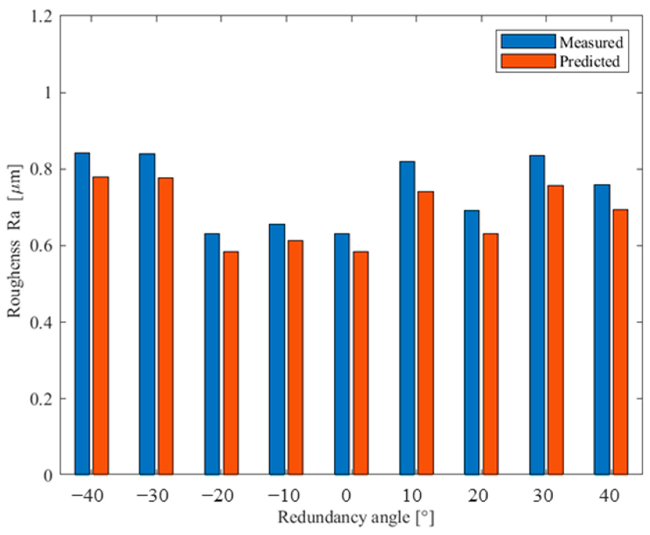
| γ | Surface Roughness within Each Measured Region (µm) | Predicted (µm) | Error (%) | |||
|---|---|---|---|---|---|---|
| 1 | 2 | 3 | Mean | |||
| −40° | 0.806 | 0.735 | 0.989 | 0.843 | 0.7786 | 7.64 |
| −30° | 0.723 | 0.878 | 0.921 | 0.841 | 0.7783 | 7.46 |
| −20° | 0.598 | 0.645 | 0.651 | 0.631 | 0.5835 | 7.53 |
| −10° | 0.481 | 0.863 | 0.622 | 0.655 | 0.6141 | 6.24 |
| 0° | 0.469 | 0.638 | 0.790 | 0.632 | 0.5848 | 7.47 |
| 10° | 0.864 | 0.856 | 0.740 | 0.820 | 0.7416 | 9.56 |
| 20° | 0.629 | 0.612 | 0.831 | 0.691 | 0.6308 | 8.71 |
| 30° | 0.999 | 0.705 | 0.802 | 0.835 | 0.7577 | 9.26 |
| 40° | 0.629 | 0.893 | 0.756 | 0.759 | 0.6952 | 8.41 |
Disclaimer/Publisher’s Note: The statements, opinions and data contained in all publications are solely those of the individual author(s) and contributor(s) and not of MDPI and/or the editor(s). MDPI and/or the editor(s) disclaim responsibility for any injury to people or property resulting from any ideas, methods, instructions or products referred to in the content. |
© 2024 by the authors. Licensee MDPI, Basel, Switzerland. This article is an open access article distributed under the terms and conditions of the Creative Commons Attribution (CC BY) license (https://creativecommons.org/licenses/by/4.0/).
Share and Cite
Liu, J.; Zhao, Y.; Niu, Y.; Cao, J.; Zhang, L.; Zhao, Y. Optimization of Redundant Degrees of Freedom in Robotic Flat-End Milling Based on Dynamic Response. Appl. Sci. 2024, 14, 1877. https://doi.org/10.3390/app14051877
Liu J, Zhao Y, Niu Y, Cao J, Zhang L, Zhao Y. Optimization of Redundant Degrees of Freedom in Robotic Flat-End Milling Based on Dynamic Response. Applied Sciences. 2024; 14(5):1877. https://doi.org/10.3390/app14051877
Chicago/Turabian StyleLiu, Jinyu, Yiyang Zhao, Yuqin Niu, Jiabin Cao, Lin Zhang, and Yanzheng Zhao. 2024. "Optimization of Redundant Degrees of Freedom in Robotic Flat-End Milling Based on Dynamic Response" Applied Sciences 14, no. 5: 1877. https://doi.org/10.3390/app14051877
APA StyleLiu, J., Zhao, Y., Niu, Y., Cao, J., Zhang, L., & Zhao, Y. (2024). Optimization of Redundant Degrees of Freedom in Robotic Flat-End Milling Based on Dynamic Response. Applied Sciences, 14(5), 1877. https://doi.org/10.3390/app14051877