Abstract
The central-symmetric time-fractional heat conduction equation with heat absorption is investigated in a solid with a spherical hole under time-harmonic heat flux at the boundary. The problem is solved using the auxiliary function, for which the Robin-type boundary condition with a prescribed value of a linear combination of a function and its normal derivative is fulfilled. The Laplace and Fourier sine–cosine integral transformations are employed. Graphical representations of numerical simulation results are given for typical values of the parameters.
1. Introduction
Fractional calculus has many advantages in various areas of investigation [1,2,3,4,5,6]. Abstract integro-differential equations have been discussed in fundamental monographs [7,8].
The classical theory of heat conduction is based on the assumption that the heat flux vector at a point at time t is proportional to the temperature gradient at the same point and at the same time t. This is the content of the standard (local) Fourier law
where k is the thermal conductivity coefficient.
The time-nonlocal generalization of the Fourier law describing “long-tail” memory is formulated as [9,10]
where is the gamma function and can be written in terms of the Riemann–Liouville time-fractional integrals and derivatives:
Here,
is the Riemann–Liouville fractional integral, and
is the Riemann–Liouville fractional derivative of order [11,12]. The Caputo fractional derivative is defined as
Recall the equations of the Laplace transform for fractional integrals and derivatives [11,12]:
where the asterisk marks the transform and s denotes the Laplace transform variable.
The constitutive equations for the heat flux (4) and (5) in combination with the law of conservation of energy lead to the time-fractional heat conduction equation with the Caputo derivative
where a can be taken as a counterpart of the thermal diffusivity coefficient, and the Caputo time-derivative is denoted as
The generalization of Equation (12)
has been considered in several publications [13,14,15,16,17,18]. Two special versions of Equation (13) with integer values of the time derivative are well known. The parabolic equation
describes, for example, bioheat transfer and lateral heat or mass exchange in a thin plate [19,20,21,22,23], whereas the hyperbolic Klein–Gordon equation
appears in quantum field theory, nonlinear optics, and solid state physics [24,25].
The solutions of the parabolic Equation (14) and time-fractional Equation (13) have different medical applications: hypothermia, ablation, thermotherapy (see, for example, [26,27,28,29,30] and the references therein).
Heat conduction in a medium with a spherical cavity was investigated in the literature under different generalized theories [31,32,33,34,35,36]. In this paper, we study the central-symmetric time-fractional heat conduction equation with heat absorption (13) in a solid with a spherical hole of radius R under time-harmonic heat flux boundary conditions. The problem is solved using the auxiliary function , for which the boundary condition of Robin type with the given boundary value of a linear combination of a function and its normal derivative is fulfilled. The Laplace and Fourier sine–cosine integral transformations are employed. Graphical representations of numerical simulation results are presented for typical values of the parameters. The present investigation extends and evolves the results of previous studies [37,38,39,40].
2. Statement and Solution of the Problem
Consider the central symmetric Equation (13) in an infinite medium with a spherical hole with radius R
with zero initial conditions
and time-harmonic heat flux at the boundary
where is a constant and denotes the angular frequency.
The zero condition at infinity is also assumed:
The auxiliary function and the auxiliary spatial variable are used. Then, instead of Equations (16)–(21), we obtain
The initial boundary value problem will be solved employing the integral transform tools. Using the rules (9)–(11), applying the Laplace transform to Equations (22)–(27) gives:
Provided the Robin boundary condition with the given boundary value of a linear combination of a function and its normal derivative, the Fourier sine–cosine transform is used [5,41]:
with the kernel
Here, the Fourier sine-cosine transform is denoted by the tilde, with being the transformation variable.
The Fourier sine–cosine transform of the second derivative of a function has the form:
Applying the Fourier sine–cosine transform with respect to the auxiliary spatial variable x to Equation (28) while taking into consideration the boundary condition (29), we get the solution in the transform domain:
Using the convolution theorem and the following formula [11,12]
where is the Mittag–Leffler function
after inverting both integral transforms, we obtain
and finally
Figure 1, Figure 2, Figure 3 and Figure 4 present the real part of the solution (39) for different values of the parameters appearing in this equation. In numerical simulations, the following non-dimensional quantities marked by the bar are used:

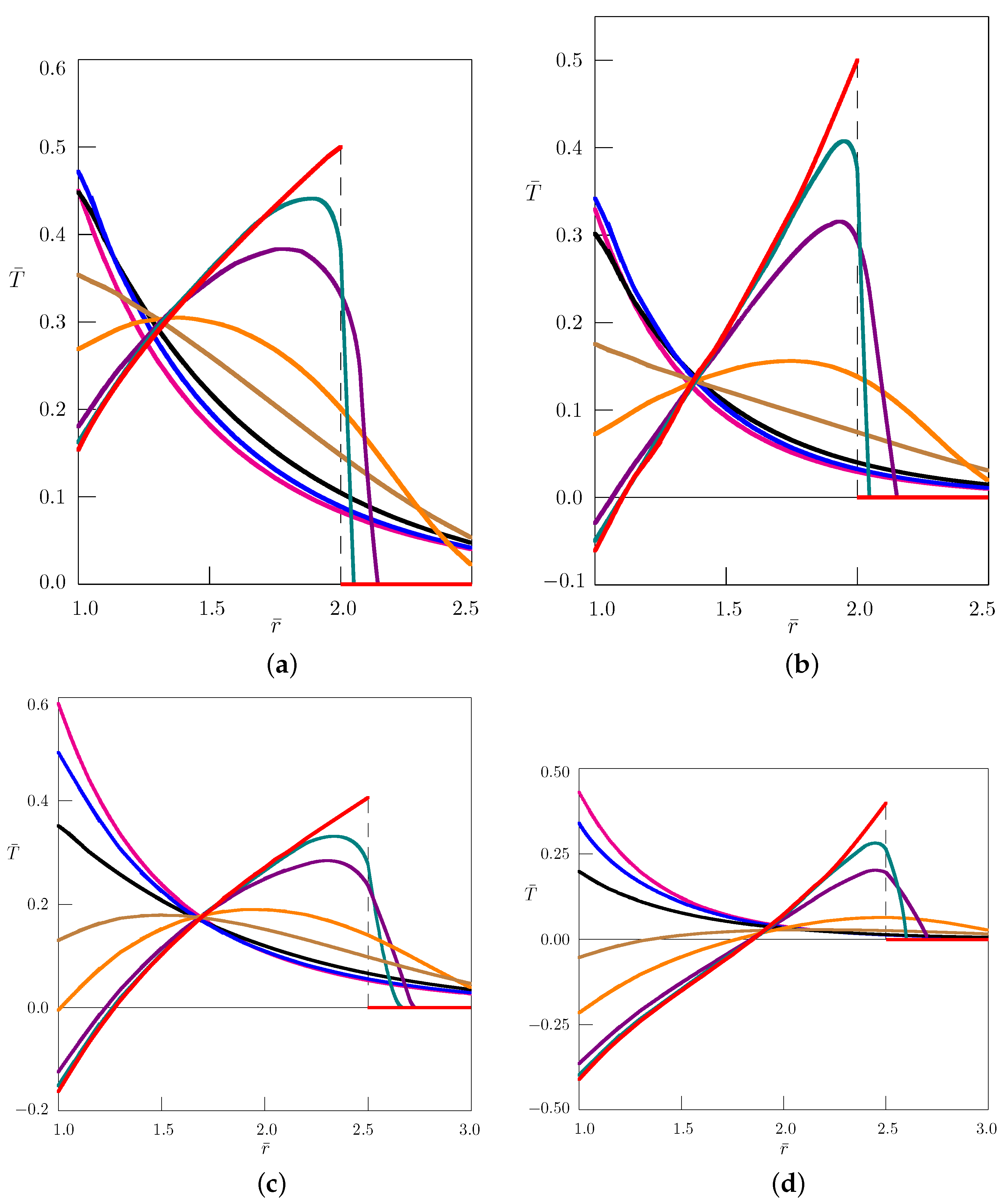
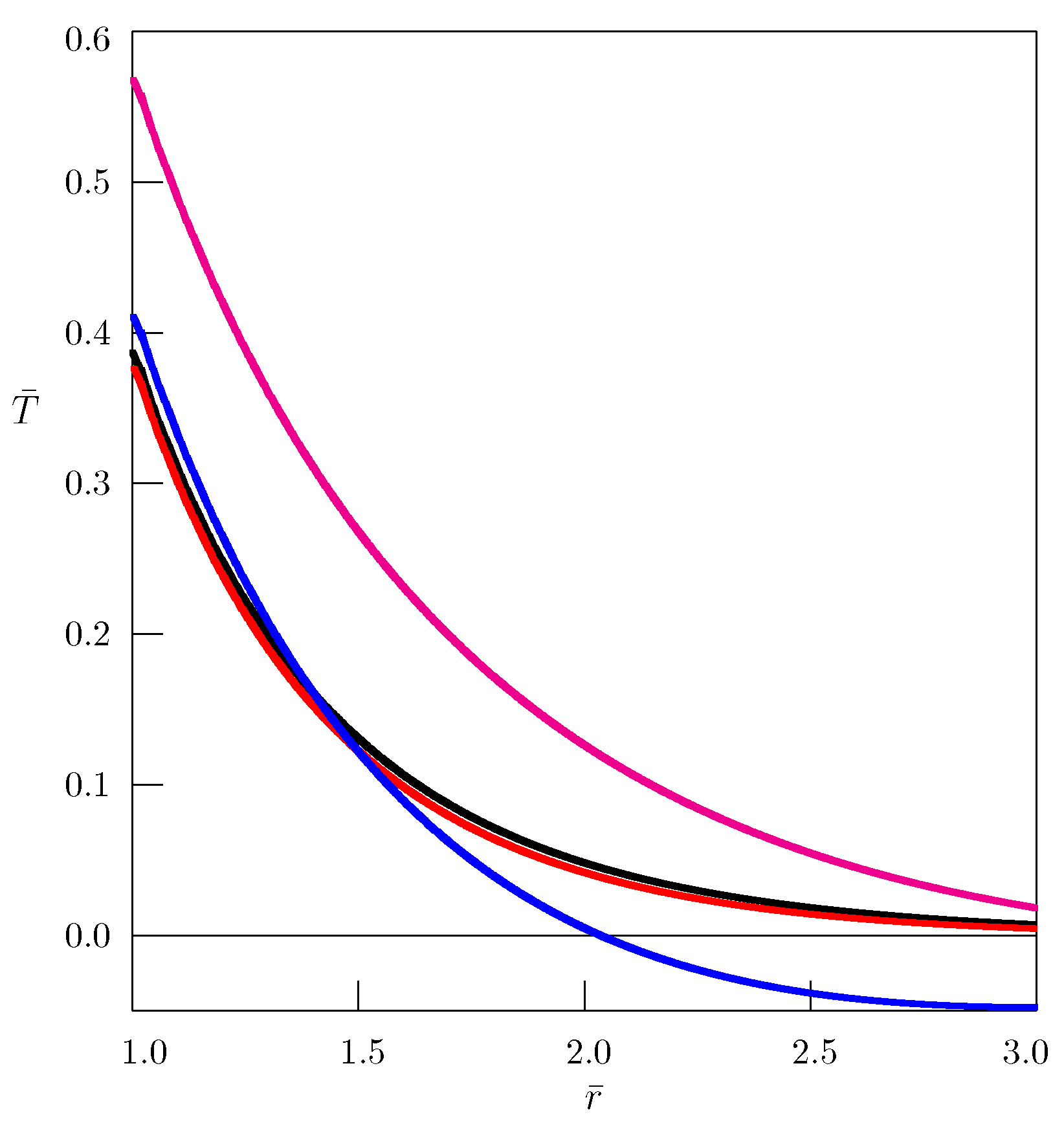
Figure 1.
Dependence of temperature on the radial coordinate . The results of computer simulations for the angular frequency and the values of parameters: , —(a); , —(b); , —(c); , —(d); —– = 0; —– = 0.5; —– = 1; —– = 1.5; —– = 1.75; —– = 1.95; —– = 1.99; —– = 2.
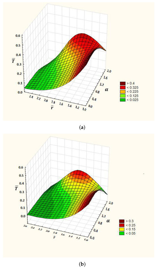
Figure 2.
Dependence of temperature on the radial coordinates and the order of fractional derivative for time and the values of the parameter: —(a); —(b).
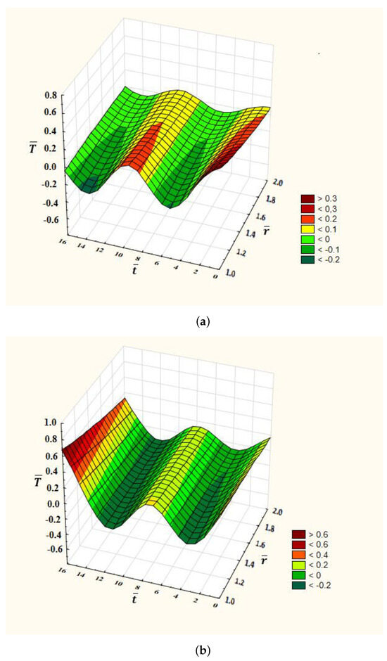
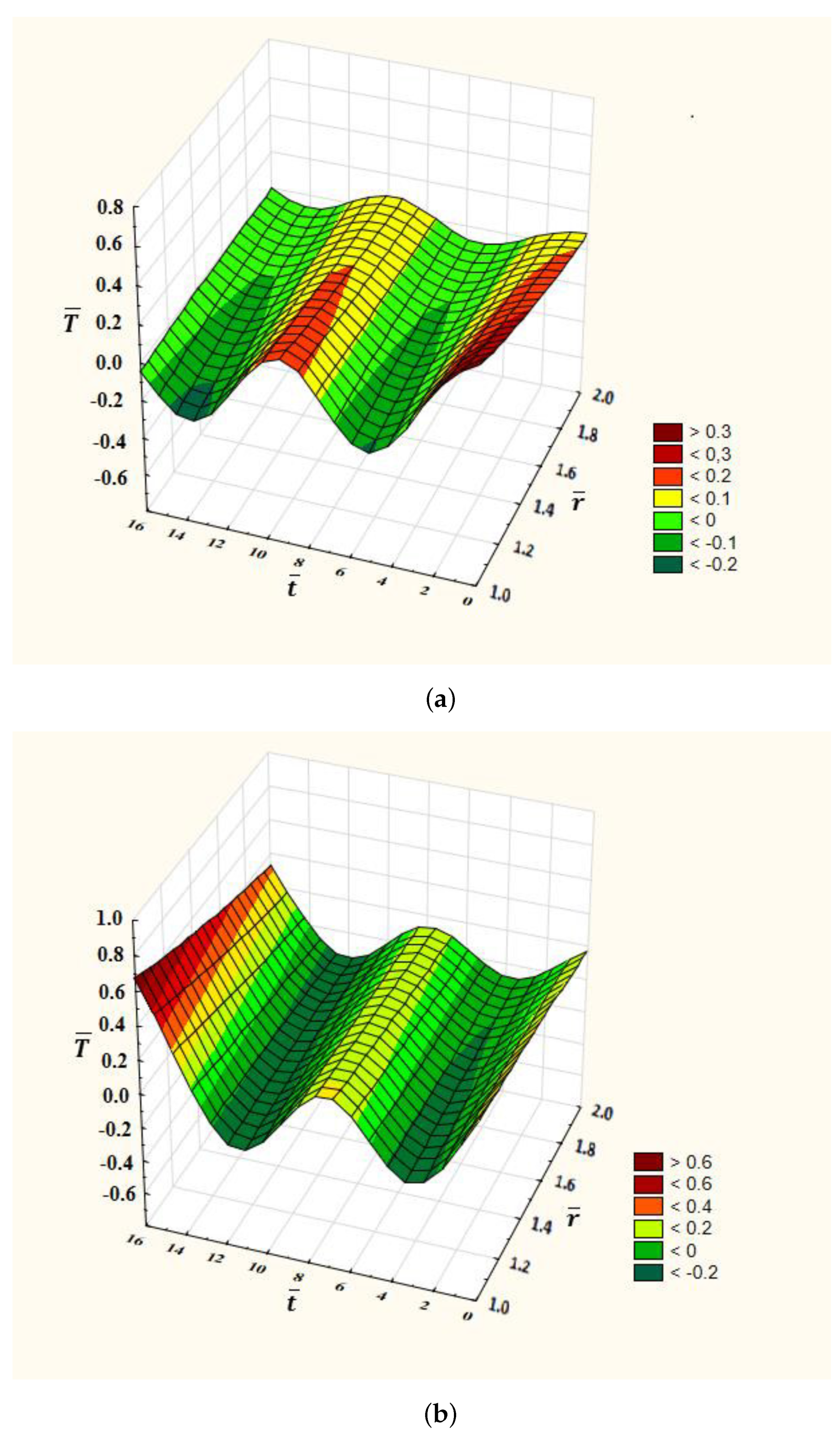
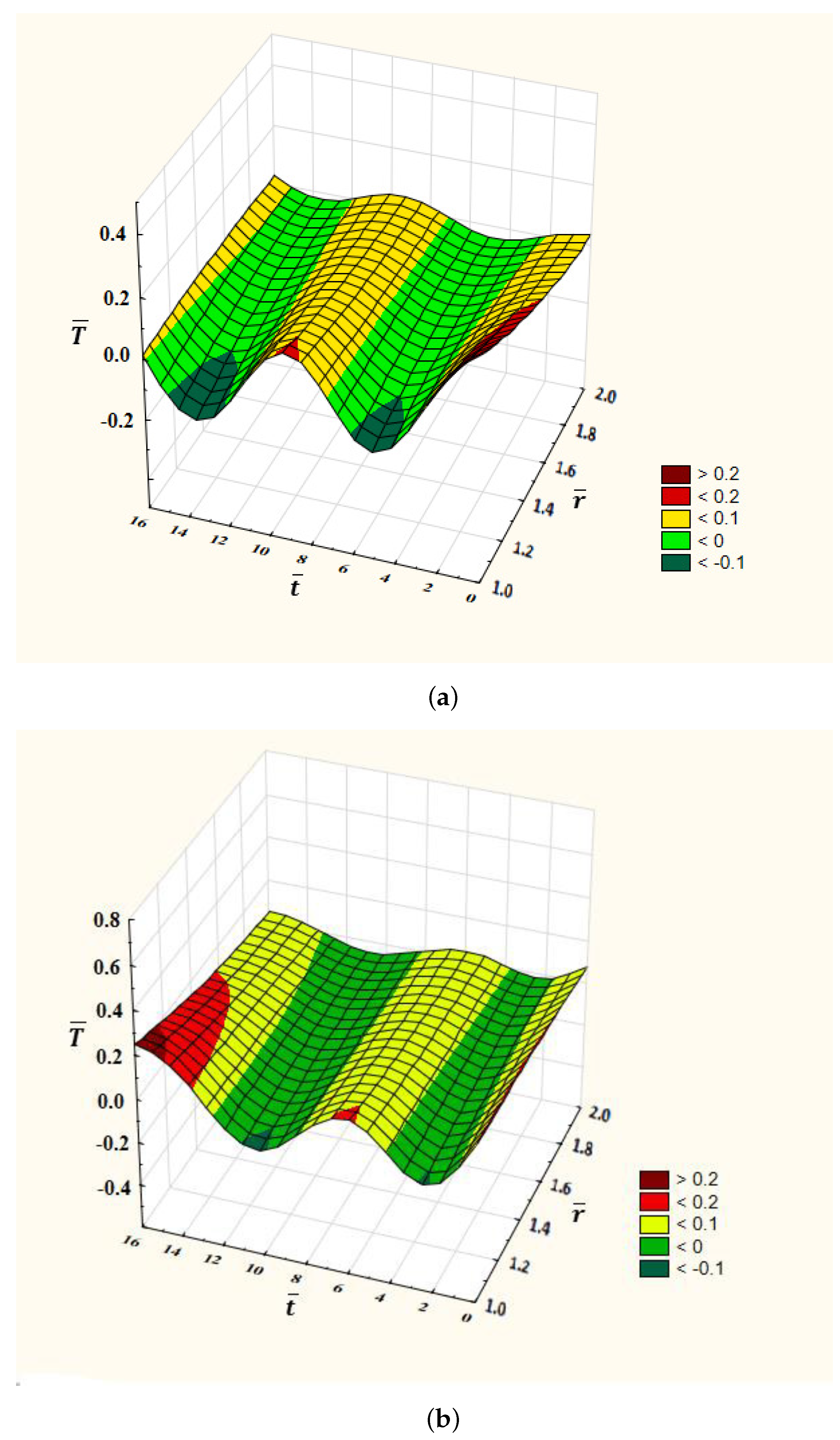
Figure 3.
Dependence of temperature on time and the radial coordinates for the angular frequency , and the order of time-fractional derivative: —(a); —(b).
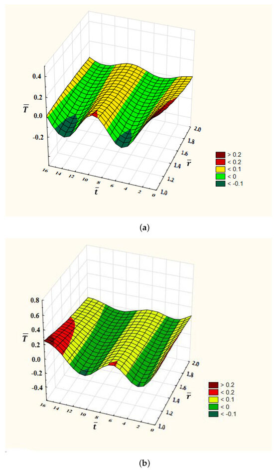
Figure 4.
Dependence of temperature on time and the radial coordinates for the angular frequency , and the order of time-fractional derivative: —(a); —(b).
3. Quasi-Steady-State Approach
In this section, we present the quasi-steady-state approach for two special cases represented by integer values of the order of time derivative. In this approach, only the boundary conditions are imposed; the initial conditions are not taken into account, but the solution is written as the product of the time-harmonic expression and unknown function of spatial variables:
3.1. Classical Heat Conduction ()
The problem is described by the equations
under the assumption
Hence,
Employing the auxiliary function and the auxiliary spatial variable , we get
The general solution of Equation (49) has the form
where the integration constants are determined from the boundary conditions (50) and (51):
The final result reads
Now, we analyze the particular case of the solution (39) for . Equation (35) for the value becomes:
and after inversion of the Laplace transform, we get
Next, we invert the Fourier sine–cosine transform and use the partial fraction decomposition
and integrals (A1)–(A4) from Appendix A. After some transformations, we obtain
where is the complementary error function.
The first summand in Equation (58) coincides with the quasi-steady-state expression (54) and the remaining terms describe the transition regime.
Figure 5 compares the real parts of the solutions (54) and (58) for the values of heat absorption parameter and .

Figure 5.
Dependence of the solution to the parabolic heat conduction Equation () on the radial coordinates. The results of computer simulations for the angular frequency and time . —– the quasi-steady-state approach for ; —– the general solution describing the transition process for ; —– the quasi-steady-state approach for ; —– the general solution describing the transition process for .
3.2. Ballistic Heat Conduction ()
The quasi-steady state approach is described by the equations
under the assumption
Hence,
Making use of the auxilliary function and the auxilliary spatial variable , we get
We confine our consideration to the case . Then,
and from the boundary conditions (67) and (68), it follows that
and consequently,
The general solution for ballistic heat conduction can be obtained from Equation (35) with :
After inverting the Laplace transform
and after evaluation of the integral in Equation (73), we obtain
Inversion of the Fourier sine–cosine transform gives
Reverting in Equation (77) to the variable r and temperature
we see that the first summand in the expression (78) coincides with the quasi-steady-state solution. For , the integrals in Equation (78) cannot be evaluated analytically and should be calculated numerically. For , the integrals in Equation (78) can be evaluated analytically using Equations (A5)–(A8) from Appendix A. In this case, Equation (78) leads to
Hence, there is the wave front at . Recall that in the Klein–Gordon Equation (59), the coefficient a can be taken as , where c is the wave velocity.
Figure 6 shows the real parts of solutions (71) and (78) taking the non-dimensional quantities (40) for .

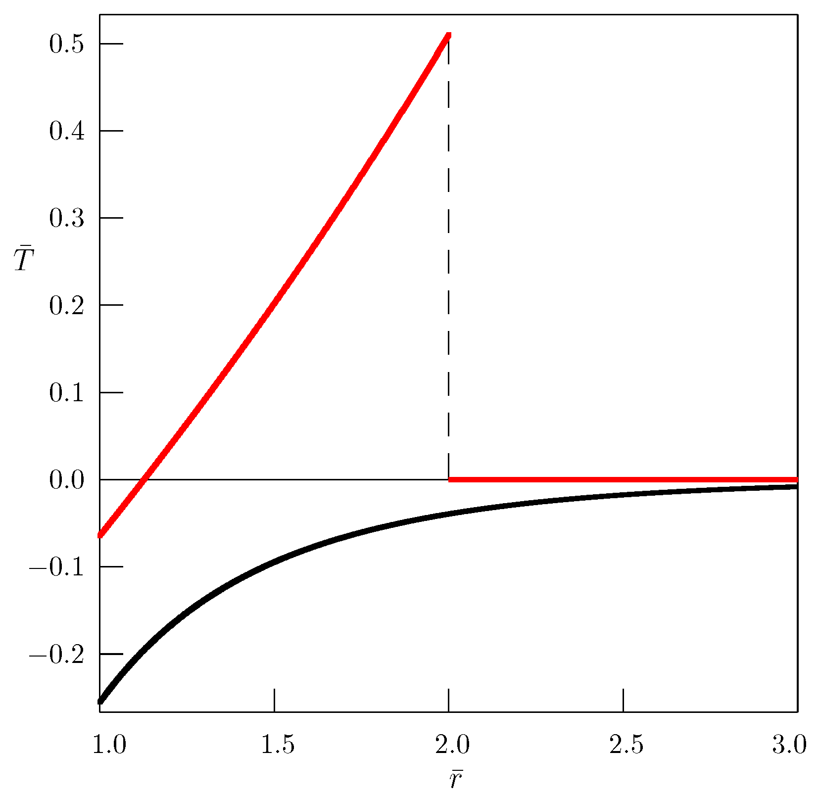
Figure 6.
Dependence of the solution to the hyperbolic Klein–Gordon Equation () on the spatial variable . The computer simulation results for the angular frequency , , and . —– the general solution describing the transition process; —– the quasi-steady-state approach (71).
4. Concluding Remarks
We have studied time-fractional heat conduction with heat absorption in an infinite medium with a spherical hole under time-harmonic heat flux at its boundary. In numerical simulations, we have utilized different values of non-dimensional parameters to show the distinguishing properties of solutions.
It should be pointed out that the quasi-steady-state approach can be considered only for integer orders of the time derivative and and cannot be studied for fractional orders of the Caputo derivative because for a non-integer [42],
It is observable from the figures that at different times, the absorption parameter can cause a change in the sign of the temperature on the cavity surface. Figure 1 shows that for , the temperature at the cavity surface is larger and for , it is smaller than that in the case of the standard heat conduction with . The situation changes and inverts at larger distances from the cavity, and there is a point at some distance where the temperature is approximately the same for all values of . In medical applications, it is possible to choose the necessary combination of the values of , b, and according to the goals of the procedure. In the literature, there is a discussion about the optimal choice of the order of the time-derivative in the fractional heat conduction model for bilayered spherical tissue in the hyperthermia experiment [43].
It is evident from Figure 5 that for the parabolic Equation (), the process is dissipative itself and the absorption parameter significantly decreases the difference between the quasi-steady-state solution and the general solution involving the transition process. In the case of the hyperbolic Klein–Gordon Equation (), the difference between the quasi-steady state approach and the general solution describing the transition regime is more visible (see Figure 6). In particular, the quasi-steady-state solution does not have a wave front. For , the wave front at (or in terms of non-dimensional quantities, at ) is also seen in Figure 1 for different values of non-dimensional time .
Our future work will focus on studying the space-time-fractional equations with the Caputo time derivative and Riesz fractional operator (fractional Laplacian).
Author Contributions
Conceptualization, Y.P. and T.K.; methodology, Y.P. and T.K.; validation, B.W.-S. and A.Y.; formal analysis, A.Y.; investigation, Y.P. and T.K.; software, T.K., B.W.-S. and A.Y.; supervision, B.W.-S.; writing—original draft preparation, T.K. and A.Y; writing—review and editing, Y.P. All authors have read and agreed to the published version of the manuscript.
Funding
This research received no external funding.
Institutional Review Board Statement
Not applicable.
Informed Consent Statement
Not applicable.
Data Availability Statement
Data are contained within the article.
Conflicts of Interest
The authors declare no conflicts of interest.
Appendix A
Integrals (A1)–(A6) used in the paper are taken from [44]:
References
- Tarasov, V.E. Fractional Dynamics: Applications of Fractional Calculus to Dynamics of Particles, Fields and Media; Springer: Berlin/Heidelberg, Germany, 2010. [Google Scholar]
- Uchaikin, V.V. Fractional Derivatives for Physicists and Engineers; Springer: Berlin, Germany, 2013. [Google Scholar]
- Herrmann, R. Fractional Calculus: An Introduction for Physicists, 2nd ed.; World Scientific: Singapore, 2014. [Google Scholar]
- Atanacković, T.M.; Pilipović, S.; Stanković, B.; Zorica, D. Fractional Calculus with Applications in Mechanics: Vibrations and Diffusion Processes; John Wiley & Sons: Hoboken, NJ, USA, 2014. [Google Scholar]
- Povstenko, Y. Linear Fractional Diffusion-Wave Equation for Scientists and Engineers; Birkhäuser: New York, NY, USA, 2015. [Google Scholar]
- Tarasov, V.E.; Tarasova, V.V. Economic Dynamics with Memory: Fractional Calculus Approach; de Gruyter: Berlin, Germany, 2021. [Google Scholar]
- Prüss, J. Evolutionary Integral Equations and Applications; Birkhäuser: Basel, Switzerland, 1993. [Google Scholar]
- Kostić, M. Abstract Volterra Integro-Differential Equations; CRC Press: Boca Raton, FL, USA, 2015. [Google Scholar]
- Povstenko, Y. Fractional heat conduction equation and associated thermal stresses. J. Therm. Stress. 2005, 28, 83–102. [Google Scholar] [CrossRef]
- Povstenko, Y. Non-axisymmetric solutions to time-fractional diffusion-wave equation in an infinite cylinder. Frac. Calc. Appl. Anal. 2011, 14, 418–435. [Google Scholar] [CrossRef]
- Podlubny, I. Fractional Differential Equations; Academic Press: San Diego, CA, USA, 1999. [Google Scholar]
- Kilbas, A.A.; Srivastava, H.M.; Trujillo, J.J. Theory and Applications of Fractional Differential Equations; Elsevier: Amsterdam, The Netherlands, 2006. [Google Scholar]
- Golmankhaneh, A.K.; Golmankhaneh, A.K.; Baleanu, D. On nolinear fractional Klein-Gordon equation. Signal Process. 2011, 91, 446–451. [Google Scholar] [CrossRef]
- Kheiri, H.; Shahi, S.; Mojaver, A. Analytical solutions for the fractional Klein-Gordon equation. Comput. Meth. Diff. Equ. 2014, 2, 99–114. [Google Scholar]
- Ferrás, L.L.; Ford, N.J.; Morgado, M.L.; Nóbrega, J.M.; Rebelo, M.S. Fractional Pennes’ bioheat equation: Theoretical and numerical studies. Fract. Calc. Appl. Anal. 2015, 18, 1080–1106. [Google Scholar] [CrossRef]
- Damor, R.S.; Kumar, S.; Shukla, A.K. Solution of fractional bioheat equation in terms of Fox’s H-Function. SpringerPlus 2016, 5, 111. [Google Scholar] [CrossRef]
- Qin, Y.; Wu, K. Numerical solution of fractional bioheat equation by quadratic spline collocation method. J. Nonlinear Sci. Appl. 2016, 9, 5061–5072. [Google Scholar] [CrossRef]
- Vitali, S.; Castellani, G.; Mainardi, F. Time fractional cable equation and applications in neurophysiology. Chaos Solitons Fractals 2017, 102, 467–472. [Google Scholar] [CrossRef]
- Pennes, H.H. Analysis of tissue and arterial blood temperatures in the resting human forearm. J. Appl. Physiol. 1948, 1, 93–122. [Google Scholar] [CrossRef]
- Gafiychuk, V.V.; Lubashevsky, I.A.; Datsko, B.Y. Fast heat propagation in living tissue caused by branching artery network. Phys. Rev. E 2005, 72, 051920. [Google Scholar] [CrossRef]
- Lakhssassi, A.; Kengne, E.; Semmaoui, H. Modifed Pennes’ equation modelling bio-heat transfer in living tissues: Analytical and numerical analysis. Nat. Sci. 2010, 2, 1375–1385. [Google Scholar] [CrossRef]
- Fasano, A.; Sequeira, A. Hemomath: The Mathematics of Blood; Springer: Cham, Switzerland, 2017. [Google Scholar]
- Polyanin, A.D. Handbook of Linear Partial Differential Equations for Engineers and Scientists; Chapman & Hall/CRC: Boca Raton, FL, USA, 2002. [Google Scholar]
- Wazwaz, A.-M. Partial Differential Equations and Solitary Waves Theory; Higher Education Press: Beijing, China; Springer: Berlin, Germany, 2009. [Google Scholar]
- Gravel, P.; Gauthier, C. Classical applications of the Klein-Gordon equation. Am. J. Phys. 2011, 79, 447–453. [Google Scholar] [CrossRef]
- Kumar, P.; Kumar, D.; Rai, K.N. Non-linear dual-phase-lag model for analyzing heat transfer phenomena in living tissues during thermal ablation. J. Therm. Biol. 2016, 60, 204–212. [Google Scholar] [CrossRef] [PubMed]
- Kumar, D.; Rai, K.N. Numerical simulation of time fractional dual-phase-lag model of heat transfer within skin tissue during thermal therapy. J. Therm. Biol. 2017, 67, 49–58. [Google Scholar] [CrossRef]
- Dutta, J.; Kundu, B. Thermal wave propagation in blood perfused tissues under hyperthermia treatment for unique oscillatory heat flux at skin surface and appropriate initial condition. Heat Mass Transfer 2018, 54, 3199–3217. [Google Scholar] [CrossRef]
- Kumar, M.; Rai, K.N. Numerical simulation of time-fractional bioheat transfer model during cryosurgical treatment of skin cancer. Comput. Therm. Sci. 2021, 13, 51–75. [Google Scholar] [CrossRef]
- Morega, A.; Morega, M.; Dobre, A. Computational Modeling in Biomedical Engineering and Medical Physics; Academic Press: London, UK, 2021. [Google Scholar]
- Mukhopadhyay, S. Thermoelastic interactions without energy dissipation in an unbounded body with a spherical cavity subjected to harmonically varying temperature. Mech. Res. Commun. 2004, 31, 81–89. [Google Scholar] [CrossRef]
- Aouadi, M. A problem for an infinite elastic body with a spherical cavityin the theory of generalized thermoelastic diffusion. Int. J. Solids Struct. 2007, 44, 5711–5722. [Google Scholar] [CrossRef]
- Liu, G.; Xie, K.; Zheng, R. Thermo-elastodynamic response of a spherical cavity in saturated poroelastic medium. Appl. Math. Model. 2010, 34, 2203–2222. [Google Scholar] [CrossRef]
- Zenkour, A.M.; Mashat, D.S.; Abouelregal, A.E. Generalized thermodiffusion for an unbounded body with a spherical cavity subjected to periodic loading. J. Mech. Sci. Technol. 2012, 26, 749–757. [Google Scholar] [CrossRef]
- Kumari, B.; Kumar, A.; Gupta, M.; Mukhopadhyay, S. Analysis of a recent heat conduction model with a delay for thermoelastic interactions in an unbounded medium with a spherical cavity. Appl. Appl. Math. 2018, 13, 863–891. [Google Scholar]
- Youssef, H.M.; Alghamdi, A.A. Influence of the fractional-order strain on an infinite material with a spherical cavity under Green-Naghdi hyperbolic two-temperature thermoelasticity theory. J. Eng. Therm. Sci. 2023, 3, 11–24. [Google Scholar] [CrossRef]
- Povstenko, Y.; Kyrylych, T. Time-fractional diffusion with mass absorption under harmonic impact. Fract. Calc. Appl. Anal. 2018, 21, 118–133. [Google Scholar] [CrossRef]
- Povstenko, Y.; Kyrylych, T. Time-fractional diffusion with mass absorption in a half-line domain due to boundary value of concentration varying harmonically in time. Entropy 2018, 19, 346. [Google Scholar] [CrossRef] [PubMed]
- Datsko, B.; Podlubny, I.; Povstenko, Y. Time-fractional diffusion-wave equation with mass absorption in a sphere under harmonic impact. Mathematics 2019, 7, 433. [Google Scholar] [CrossRef]
- Povstenko, Y.; Kyrylych, T. Axisymmetric fractional diffusion with mass absorption in a circle under time-harmonic impact. Entropy 2022, 24, 1002. [Google Scholar] [CrossRef]
- Galitsyn, A.S.; Zhukovsky, A.N. Integral Transforms and Special Functions in Heat Conduction Problems; Naukova Dumka: Kiev, Ukraine, 1976. (In Russian) [Google Scholar]
- Povstenko, Y. Fractional heat conduction in a space with a source varying harmonically in time and associated thermal stresses. J. Therm. Stress. 2016, 39, 1442–1450. [Google Scholar] [CrossRef]
- Yu, B.; Jiang, X. Temperature prediction by a fractional heat conduction model for the bilayered spherical tissue in the hyperthermia experiment. Int. J. Therm. Sci. 2019, 145, 105990. [Google Scholar] [CrossRef]
- Erdélyi, A.; Magnus, W.; Oberhettinger, F.; Tricomi, F. Tables of Integral Transforms; McGraw-Hill: New York, NY, USA, 1954; Volume 1. [Google Scholar]

Disclaimer/Publisher’s Note: The statements, opinions and data contained in all publications are solely those of the individual author(s) and contributor(s) and not of MDPI and/or the editor(s). MDPI and/or the editor(s) disclaim responsibility for any injury to people or property resulting from any ideas, methods, instructions or products referred to in the content. |
© 2024 by the authors. Licensee MDPI, Basel, Switzerland. This article is an open access article distributed under the terms and conditions of the Creative Commons Attribution (CC BY) license (https://creativecommons.org/licenses/by/4.0/).