Enhancing Dehumidification in the Cable Room of a Ring Main Unit through CFD-EMAG Coupling Simulation and Experimental Verification

Abstract

The cable room, located at the base of the ring main unit, is prone to water vapor due to its proximity to damp cable holes and its relatively enclosed structure. This may penetrate internally and ultimately affect operational safety. Therefore, a dehumidifier was introduced to utilize dry air for internal circulation. To enhance the dehumidification in the cable room, the cable room device was designed for experimental research. Meanwhile, computational fluid dynamics (CFD)-electromagnetic (EMAG) coupling simulation is used to calculate the power loss of heat sources and their influence on multiple physical fields in numerical simulations. The feasibility of this study was confirmed by comparing the relative humidity, temperature, and velocity values between the experimental and numerical approaches. Furthermore, the layout of the ventilation pipes was modified to a vertical distribution, with upward supply and downward suction, to improve the airflow. The results indicate that the maximum relative errors in temperature, relative humidity, and velocity are only 3.61%, 7.14%, and 7.14%, respectively, which fall within an acceptable range. On this basis, additional simulation analysis was conducted on the humidity, dew point temperature, and airflow within the cable room, using an optimized model with a more comprehensive internal structure and cables. After implementing an optimized ventilation pipe layout, the relative humidity at the corresponding measuring points can decrease by up to 10.6%. The dew point temperature has decreased by 2.61 °C and the airflow has become more stable.

1. Introduction

The ring main unit (RMU) is considered the primary distribution device in modern power systems [1]. The device also plays a significant role in stabilizing the system by controlling and protecting the power supply [2]. The reliability and stability of power equipment are crucial in outdoor electrical engineering. However, fluctuations in internal temperature and humidity can easily impact the maintenance and operational safety of the system, making reliable equipment crucial. For instance, if the surface temperature of the inner wall of metal equipment drops below the dew point temperature, water droplets will condense on the surface, leading to the corrosion of the metal components and a reduced insulation performance. This increases the risk of equipment arcing or breakdown, potentially resulting in safety accidents [3]. Therefore, preventing the aforementioned condensation phenomenon is crucial for the safety of the power system.

According to [4], the occurrence of condensation mainly depends on the relative humidity, temperature, and dew point temperature in the cabinet. Many studies have focused on explorative measures and preventive measures for condensation, combined with the causes, conditions, and hazards of high condensation pressure in cabinets, and proposed some technical measures to prevent condensation [5,6,7]. Ventilation holes are suggested to be added around the foundation of the RMU to solve this problem by reducing the humidity in the air [8]. However, increasing only ventilation holes without adding dehumidifiers results in limited dehumidification efficiency.

To reduce condensation, cabinets are usually equipped with dehumidifiers. Traditional dehumidifiers are divided into heating dehumidifiers and condensing dehumidifiers, but both dehumidification methods have obvious drawbacks. A method combining electric heating and an anti-condensation controller has been proposed for dehumidification and anti-condensation in 12 kV switchgear. Although the internal surface temperature increases and the relative humidity of the air decreases, condensation cannot be completely prevented. The position of the heater also has a significant impact on the dehumidification [9]; from another perspective, currently condensing dehumidifiers mainly use semiconductor refrigeration technology to reduce the temperature in humid air, and then condense the water vapor into water droplets, which are discharged from the switchgear to achieve the purpose of dehumidification [10]. However, the semiconductor condensation dehumidification method is only applicable to areas with slow environmental temperature changes.

In addition, the above two traditional methods did not consider the impact of ventilation. Research based on the projects encountered is conducted, which adopts a different method of dry air dehumidification to enhance anti-condensation. By installing inlet and outlet air ducts on the wall of the cable room of the RMU, the dehumidifier introduces dry air from the inlet duct and discharges the humid air inside the cabinet from the outlet duct, forming a good ventilation cycle to achieve the purpose of dehumidification. The different supply air temperatures and flow rates of dehumidifiers may affect the dehumidification. Using ANSYS Fluent 14 to simulate the flow field and thermal environment inside the cabinet is an effective model. Many studies use software for numerical simulation to accurately calculate the fluid flow and thermal field inside the cabinet. The ANSYS Maxwell 15 has been used to investigate the impact of copper resistivity on power loss in low-voltage switchgear [11]. Numerical simulation was conducted on switchgear to study the condensation phenomenon of humid air in switchgear under different relative humidity and boundary conditions [12]. Some studies have explored the use of the finite element analysis software Ansys 2015 to simulate the airflow field inside an outdoor ring-shaped main cabinet, and studied the effects of wind speed, shell size, and vent shape on ventilation effectiveness [13]. A measurement method has been developed for optimizing the temperature fluid flow field by considering grid control, boundary conditions, and heat sources as switch devices [14]. However, only a few recent studies have addressed the mechanical flow characteristics in RMUs [15]. Research has shown that different airflow distributions can be analyzed through numerical simulation of the thermal and humidity environment inside the switchgear [16]. However, due to its simplified structure, there was a lack of consideration for the heat source inside the room. Following this, Figure 1 illustrates the entire research process, focusing on two parts: experimental and simulation.

The novelty of this paper lies in using CFD-EMAG coupling simulation to study the distribution of multiple physical fields inside a cable room and providing support for the research through mutual verification between experiments and simulations. Based on experiments and simulations, optimized dehumidification methods and measures have been proposed, providing support for their safe operation. A simulation model containing cables was established for the CFD-EMAG coupling simulation, taking into account the unique cable compartment structure inside the RMU. Since the cable room cannot be opened for data collection after it is put into operation, a cable room device was made for a dehumidification experiment. Electric heating wires were used as heat sources to replace cables and influence the temperature and humidity fields. At the same time, a simplified simulation model containing electric heating wires was also established for comparison with the experiment. The accuracy was enhanced through mutual verification via experiments and simulations, and the pipeline layout was improved to achieve a more uniform internal gas flow. Based on this, and the literature [17,18,19], references have been provided for the cable structure, materials, and humidity settings inside the cable room, and the anti-condensation and gas flow distributions of the dehumidification method in the cable room were further simulated using a more comprehensive cable-containing model with a complete internal structure. Through experimental verification and analysis, optimization measures have been proposed to prevent condensation in cable rooms.

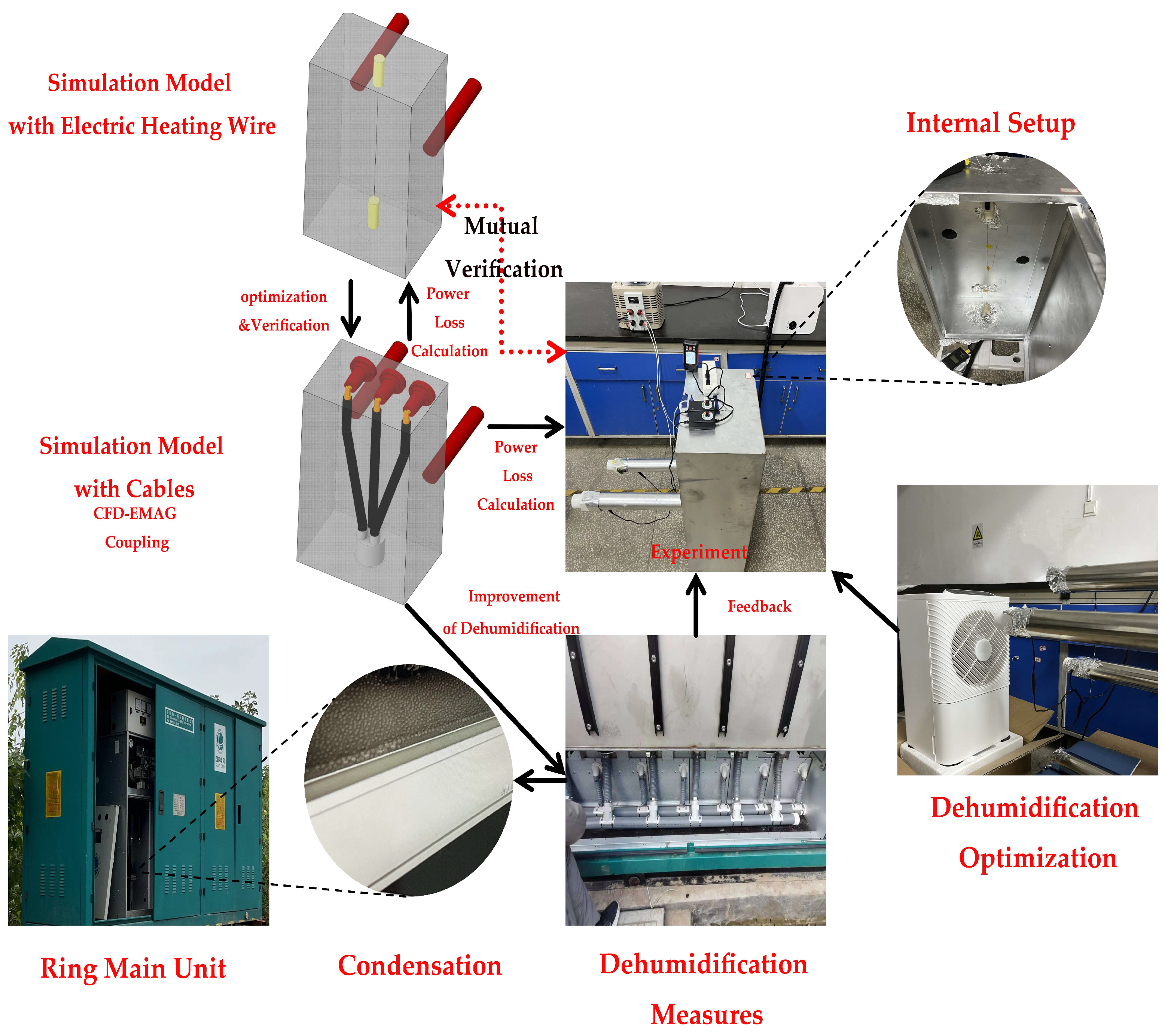
2. Materials and Methods

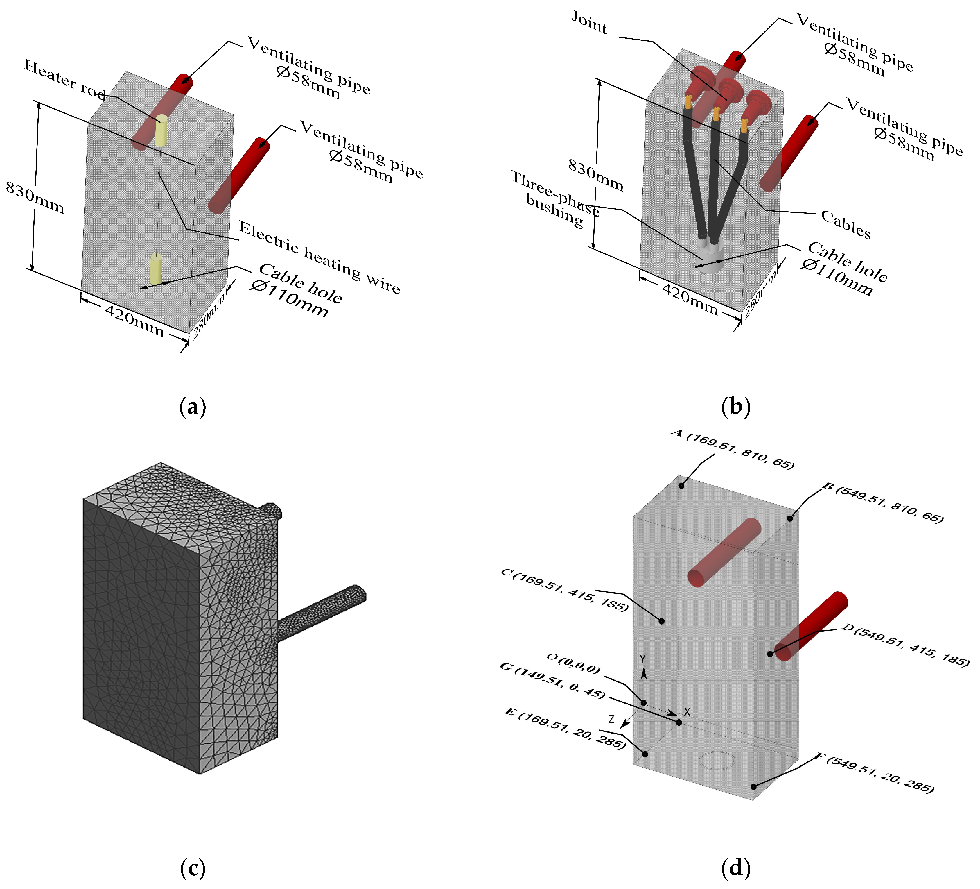
2.1. Structure and Modeling of the RMU

Based on the “10 kV AC outdoor box-type switchgear” commonly found in communities and along streets in China, a simplified model of its cable room was studied. The model has dimensions of 420 mm in length, 280 mm in width, and 830 mm in height. The dehumidifier has been simplified and is now represented by two ventilation pipes for the entry and exit of dry air. Each pipe has a length of 348 mm and a diameter of 58 mm, and they are connected to the back of the cable room. The geometric model and dimensions of the simplified cable room model with an electric heating wire are illustrated in Figure 2a. According to the configuration of the 10 kV RMU, three-phase copper core cables are chosen. In the cable room, 4.5 mm thick cross-linked polyethylene is used to create three single-phase cables, each with a radius of 11.9 mm [17]. The length of the middle cable is 565 mm, while the lengths of the left and right cables are slightly longer, approximately 570 mm. Additionally, to experimentally validate the simulation’s accuracy and assess the feasibility of the experiment, a simple cable room was constructed in a 1:1 ratio. An electric heating wire was used as the heat source for thermal analysis instead of a central cable. The wire had a length of 565 mm and a radius of 0.5 mm. Corresponding simulations were conducted to validate the results. Based on the verification results, the structure and dimensions of the simulation model with cables are depicted in Figure 2b. Due to experimental limitations, it is difficult to directly validate the case presented in Figure 2b in the laboratory. In Figure 2b, the simulation first calculates the heating power of the cable, and then adds it to the case in Figure 2a. The further optimization of the case in Figure 2b is supported through mutual verification between experiments and the case in Figure 2a. Finally, Figure 2c depicts the model grid, which will be explained in Section 2.2, while Figure 2d illustrates the positions and coordinates of the monitoring points in the model, which will be discussed in Section 2.5.

Optimization of pipe layout is one of the main optimization methods in this study. The layout of the left and right pipes is based on the original structure of the dehumidification equipment, and the pipes are located in the middle of the wall, which is referred to as Layout 1 in the following text. We are considering the layout of the cable room structure and attempting to improve it on the basis of the original layout to make the internal flow more uniform and sufficient, in order to improve the dehumidification. The schematic diagram of the pipeline layout is shown in Figure 3a,b, which includes Layout 2: exchanging the air supply and air outlet on the basis of Layout 1; Layout 3: vertically arranging ventilation ducts, taking into account the internal structure of the original cable room, adjusting the position appropriately, with the lower ducts supplying air and the upper ducts extracting air; and Layout 4: swapping the air supply and air outlet on the basis of Layout 3.

Pipes 1 and 2 are separated on the right and left sides, while pipes 3 and 4 are vertically distributed on the wall, one above the other. The layout is referred to as Layout 1, where air is supplied through Pipe 1 and extracted through Pipe 2. Layout 2 supplies air to Pipe 2 and extracts air from Pipe 1. Layouts 1 and 2 are depicted in Figure 3a. Layout 3 supplies air to Pipe 4 and extracts air from pipe 3; Layout 4 supplies air to Pipe 3 and extracts air from Pipe 4. Layouts 3 and 4 are shown in Figure 3b.

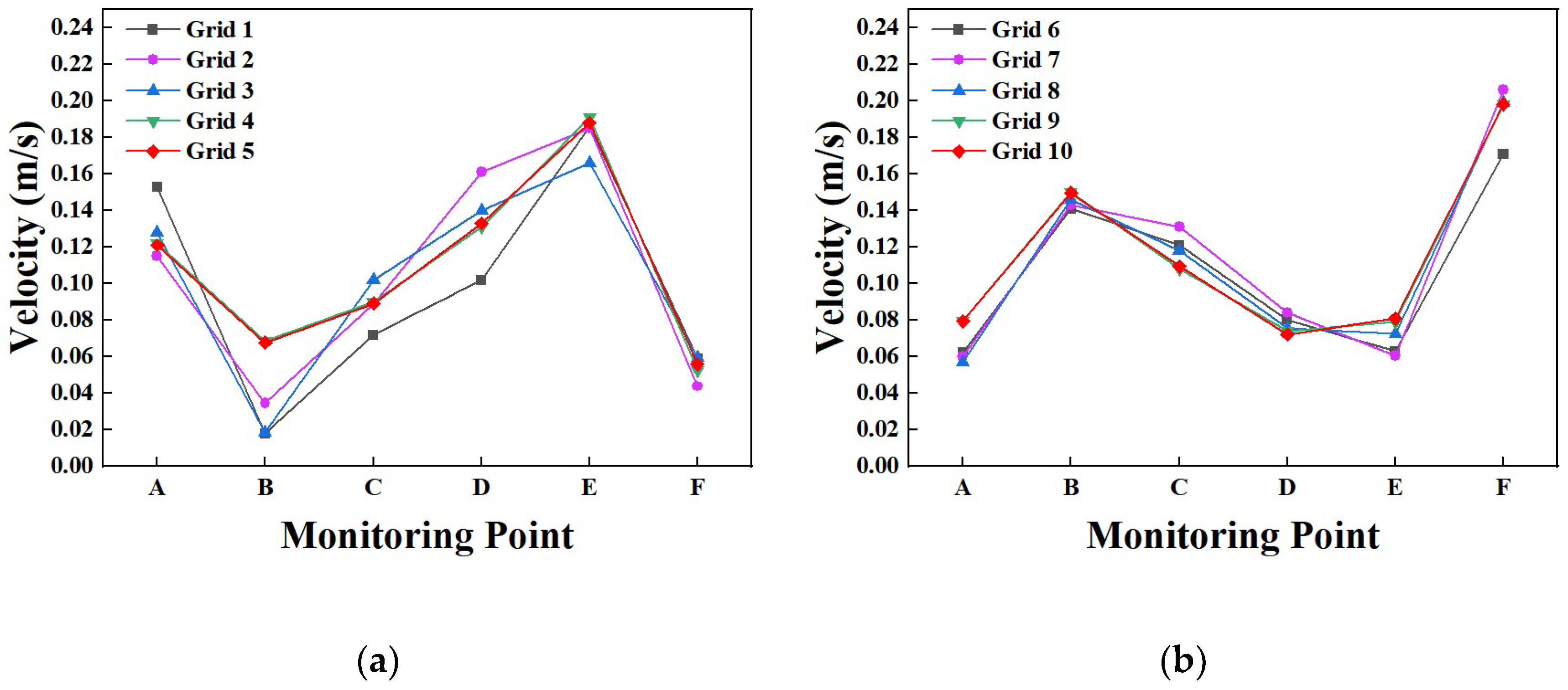
2.2. Simulation Grid

The model is divided into unstructured grids using Ansys meshing, with a total of 1,533,790 and 919,621 grids corresponding to the simulation model and a simplified model of the cable room in the validation experiment. The schematic diagram of the main grid of the cable compartment is shown in Figure 2c.

2.3. Governing Equations

2.3.1. Mathematical Model of Flow Field

In fluent simulation, the steady-state calculation of the fluid module is mainly based on the rotational flow inside the box when dry air is introduced into the secondary chamber by the dehumidifier. Therefore, a realizable $k-\epsilon$ model is used. The model should include gravity conditions according to the actual situation. The main governing equations of its mathematical model can be described as:

$$\frac{\partial \rho }{\partial t}+\rho (u\cdot \nabla )u=\nabla \cdot \left[-pI+\left(\mu +{\mu }_T\right).\right.\left.\left(\nabla u+(\nabla u{)}^T\right)\right]+F+\rho g,$$

(1)

$$\frac{\partial \rho }{\partial t}+\rho \nabla \cdot (u)=0,$$

(2)

$$\frac{\partial (\rho k)}{\partial t}+\rho (u\cdot \nabla {)}_{\mathrm{k}}=\nabla \cdot \left[\left(\mu +\frac{{\mu }_t}{{\sigma }_k}\right){\nabla }_{\mathrm{k}}\right]+G_k-\rho \epsilon ,$$

(3)

$$\frac{\partial (\rho \epsilon )}{\partial t}+\rho (u\cdot \nabla {)}_{\mathsf{\epsilon }}=\nabla \cdot \left[\left(\mu +\frac{{\mu }_t}{{\sigma }_{\epsilon }}\right){\nabla }_{\mathsf{\epsilon }}\right]+\rho C_{1}E\epsilon -\rho C_2\frac{{\epsilon }^2}{k+\sqrt{\nu \epsilon }},$$

(4)

where ρ, t, $u$, $p$, g, I, $\mu$, $T$, $F$, $k$, $\epsilon$, and $G_k$ are the density, the time, the vector, the pressure, the gravitational constant, the identity matrix, the fluid dynamic viscosity, the temperature, the volume force vector, the kinetic energy of the flow field, the dissipation rate of the flow field, and the generation term of turbulent kinetic energy k caused by buoyancy, respectively; ${\sigma }_k$, ${\sigma }_{\epsilon }$, $C_1$, E, and $C_2$ are all empirical constants.

2.3.2. Heat Conduction Model

Considering the heat exchange inside and outside the RMU, the energy equation is selected, and its mathematical model is:

$$\frac{\partial (\rho E)}{\partial t}+\nabla \cdot \left(u_i\left(\rho E+p\right)\right)=\nabla \cdot \left[k_{eff}\nabla T-{\sum }_j{h}_j{J}_j+ u_j{\left({\tau }_{ij}\right)}_{eff}\right]+S_h,$$

(5)

where E, $k_{eff}$, h, $J_j$, $\tau$, and $S_h$ are the energy, the effective heat transfer coefficient, the apparent enthalpy of an ideal gas, the diffusion flow rate of component, the shear stress, and the customize source items for users, respectively.

2.3.3. EMAG Model

The electromagnetic process of the preliminarily considered cable is described by Maxwell equations to describe the generation of power loss.

$$\nabla \cdot \mathit{H}=\mathit{J}+\frac{\partial \mathit{D}}{\partial t},$$

(6)

$$\nabla \cdot \mathit{E}=-\frac{\partial \mathit{B}}{\partial t},$$

(7)

$$\nabla \cdot \mathit{D}={\rho }_{den},$$

(8)

$$\nabla \cdot \mathit{B}=0,$$

(9)

where $\mathit{H}$, $\mathit{J}$, $\mathit{D}$, $\mathit{E}$, $\mathit{B}$, and ${\rho }_{den}$ are the magnetic filed intensity vector, the total current density vector, the electric field intensity vector, the magnetic induction vector, and the charge density, respectively.

2.4. Physical Properties and Boundary Conditions

The boundary conditions of this model mainly include the following factors: external atmospheric pressure, flow rate, temperature, outlet gauge pressure of the dehumidifier in and out of the dry air pipeline, bottom humidity source temperature, humidity, and flow rate, as well as the cable room heat transfer coefficient of the RMU model.

In the boundary condition setting in the simulation, the viscous model selects the k-epsilon realizable model, and the enhanced wall function EWF is turned on. The bottom humidity source uses a velocity inlet, with an area equivalent velocity set to 0.4 m/s, and a relative humidity set to 75%, 80%, 85%, and 100%, depending on the situation. The air supply duct velocity is set to 1.5 m/s, and after dehumidification by a dehumidifier, the relative humidity is set to 48% and the temperature is 29 °C. The outlet pressure is set to −0.91 Pa and the temperature is 28 °C; a 1.0 mm electric heating wire is used as an internal heat source to achieve a steady-state average temperature of 100 °C under fully enclosed conditions. According to [18], the heat transfer coefficient was 9.445 W/(m².K). The shear condition should be no-slip. The specific physical parameters and boundary conditions are shown in

Table 1. Boundary conditions are set.

Boundary Condition	Type	Value
Solution domain	Fluent/Maxwell	/
Fluid	Air	/
Solid 1	Copper	Thermal conductivity: 387.6 W/(m K); Bulk conductivity: 58,000,000 siemens/m;
Solid 2	Ni-Cr	Thermal conductivity: 15 W/(m K);
Solid 3	Epoxy resin	Thermal conductivity: 0.276 W/(m K);
Solid 4	Steel	Thermal conductivity: 10.27 W/(m K);
Solid 5	Cross-linked polyethylene	Thermal conductivity: 0.29 W/(m K);
Mixture	Water-vapor; Air	/
Wall	Convection	heat-transfer coefficient: 9.445 W/(m2K)
Inlet	Velocity-inlet 1; Velocity-inlet 2	Velocity: 1.5 m/s, Temperature: 29 °C, Component mass fraction (H2O): 0.01204; Velocity: 0.4 m/s, Temperature: 28 °C, Component mass fraction (H2O):0.01791/0.01904/0.02038/2387
Outlet	Pressure outer	−0.91 Pa, backflow temperature: 28 °C
Target residual	/	10−4

.

Additionally, for the sake of simplicity, certain assumptions are made: the heat release of components in the cable compartment other than cables or heating wires is neglected; the structure and heat release of three-phase cables that have not been separated are also neglected; the reverse effect of temperature on conductivity in Maxwell is not being considered in current research.

2.5. Grid Independence Verification

Five different grids are selected for each of the two models in the validation experiment. The corresponding grids for the cable room model with an electric heat wire are as follows—Grid 1: 1,177,001, Grid 2: 1,225,717, Grid 3: 1,358,326, Grid 4: 1,533,790, and Grid 5: 1,600,172. The cable room model with cables includes Grid 6: 782,880, Grid 7: 816,663, Grid 8: 831,633, Grid 9: 919,621, and Grid 10: 935,666. Six monitoring points are positioned along the XYZ coordinate axis in the cable room, as shown in Figure 2d. The measurement points A (169.51, 810, 65) and B (549.51, 810, 65) are located near the rear of the cable room at the top. Measurement points C (169.51, 415, 185) and D (549.51, 415, 185) are situated at the midpoint of the walls on opposite sides of the cable room. Measurement points E (169.51, 20, 285) and F (549.51, 20, 285) are situated near the main door at the bottom. The velocity variation trend of monitoring points in different grids is shown in Figure 4a,b. It can be observed that the velocity change trend is consistent across all detection points in various grids. In Figure 4a, when utilizing Grid 4 and Grid 5, and in Figure 4b on the right, using Grid 9 and Grid 10, the numerical stability is adequate to fulfill the calculation requirements. This confirms that the calculation results are independent of the grid.

3. Experimental Results and Simulation Analysis

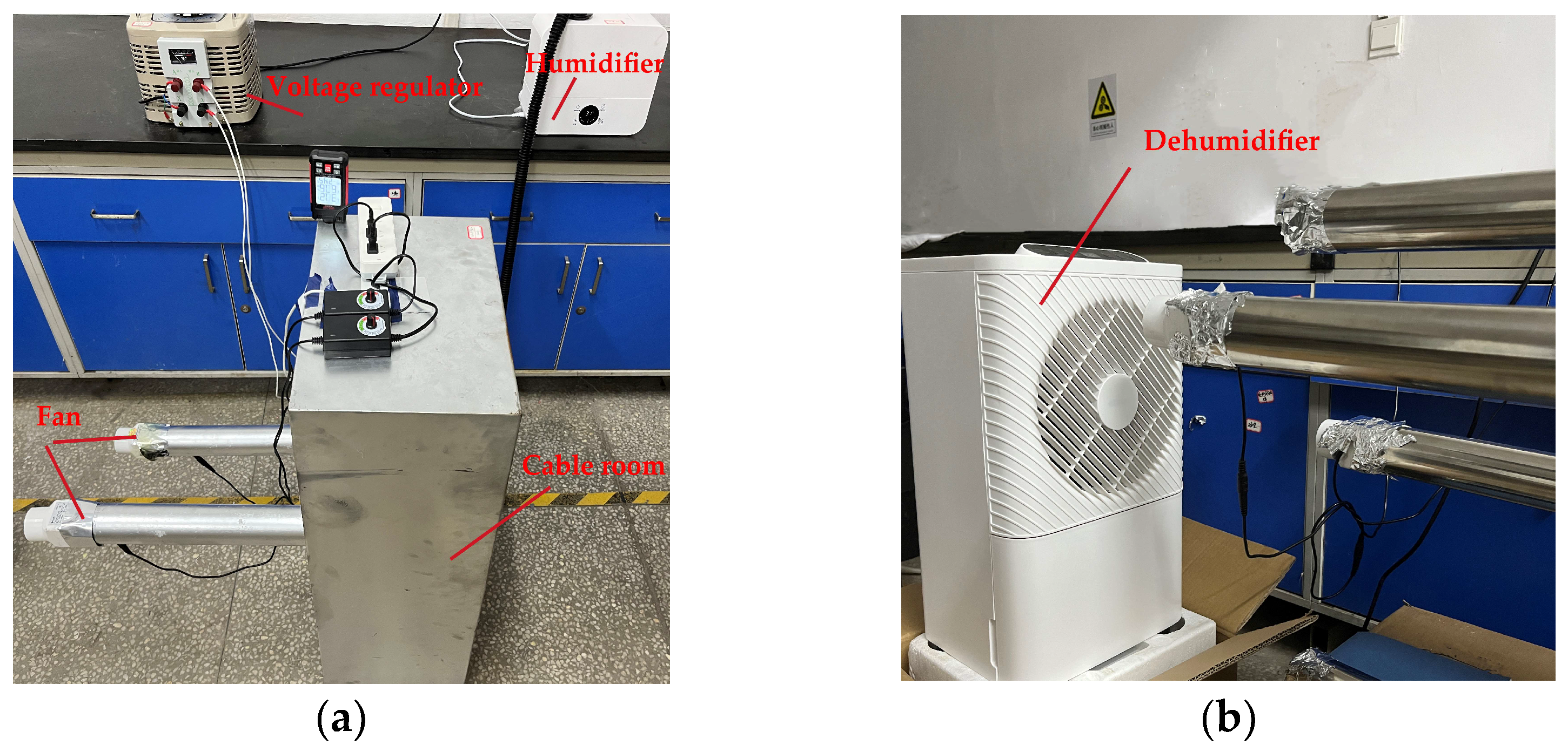
3.1. Experimental Conditions

The laboratory was kept at a room temperature of 28 °C, and the humidity was controlled at 50% for the experiment. A 1.0 mm diameter electric heating wire was placed vertically inside the cable room for temperature field research. Based on the simplified cable room model, a 630 A current excitation is applied to three individual cables, resulting in thermal powers of 4.98 W, 4.94 W, and 4.98 W, totaling 14.88 W. In total, 4.94 W of power was applied to the middle cable of the electric heating wire through a voltage regulator. When the cable room door was kept closed, the average temperature of the electric heating wire, as measured by the K-type thermocouple, was 100 °C. Figure 5a shows the initial experimental cable compartment and related equipment during the preliminary experiment. On this basis, two ventilating pipes were added, doubled in length for better measurement, and a dehumidifier was placed in front of the air supply pipeline, as shown in Figure 5b. The positions of the experiments corresponding to the above six points are depicted in Figure 6a. Moreover, as shown in Figure 6b, after doubling the length of the pipes, a hole was opened in the middle to facilitate the measurement and verification of inlet and outlet velocity values, such as G, H, I, and J.

The detailed descriptions and uncertainties of the experimental equipment are shown in

Table 2. Summary table of experimental equipment.

Equipment	Parameter	Measuring Accuracy
experimental cable room	420 × 280 × 830 mm	/
electric heating wires	Length: 565 mm Radius: 0.5 mm	/
humidifier	Evaporation capacity: 200 mL/h, Power: 28 W,	/
single-phase voltage regulator	Voltage: 220 V Power: 5000 W	/
12 L drying dehumidifier	Power: 230 W Dehumidification capacity: 0.29 kg/h Maximum air volume: 100 m3/h	/
pipeline axial flow fan	Power: 6 W, Maximum air volume: 36 m3/h	/
K-type thermocouple	Measuring range: −200 °C~+1372 °C	Temperature Accuracy: ±0.2% + 0.7 °C
anemometer	Use range: 0~0.99 m/s	Velocity accuracy: ±0.02 m/s
pressure gauge	Use range: 0~10 Pa	Pressure accuracy: ±0.1 Pa
hygrothermograph	Temperature range: −20~60 °C Humidity range: 0~100% Dew point temperature range: −50 °C~60 °C	Temperature accuracy: ±1.5 °C; Humidity accuracy: ±3.0%; Dew point temperature accuracy: ±1.5 °C

.

Experimental setup:

Before the experiment, the gaps were sealed in the door of the experimental cable room with tin foil. The electric heating wire was adjusted to a stable temperature through a voltage regulator; a certain temperature and humidity (28 °C, 50%) were maintained in the laboratory; the humidifier humidified the enclosed cable room through a pipe from the bottom (the humidity at the nozzle is approximately 100%), and then the supply and exhaust fan were turned on. In front of the air supply fan, the dehumidifier was opened to dry the air, and the airflow of the dehumidifier was controlled to be much greater than that of the fan to avoid affecting the flow rate inside the pipe; the corresponding temperature, relative humidity, velocity, and pressure data at the six monitoring points on the selected cabinet and the monitoring points on the supply and exhaust duct after stabilization were measured. At the same time, the average temperature of the electric heating wire after stabilization using a k-type thermocouple was measured. Lastly, the data were arranged and examined.

Measurement uncertainties:

Slow changes in indoor temperature and humidity; random variation in repeated measurements under the same conditions; measuring devices; measurers; and the measurement sample may not fully represent the defined object being measured.

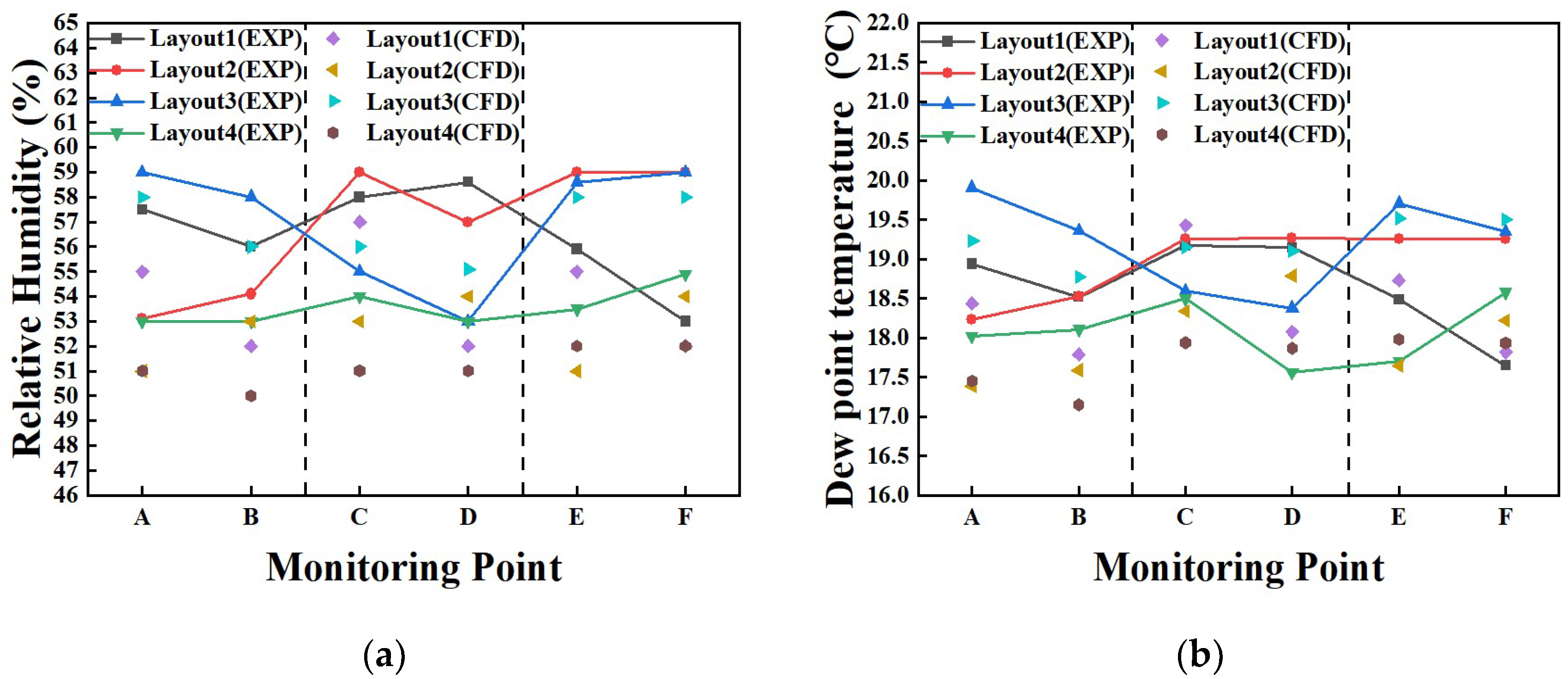
3.2. Experimental and Simulation Analysis

The data between simulation and experiment was compared, and the overall variations in temperature, relative humidity, and velocity among the six monitoring points were analyzed.

Table 3. Comparison of temperature data between experimental and simulated monitoring points for each layout.

Points	Layout 1				Layout 2				Layout 3				Layout 4
	Temperature				Temperature				Temperature				Temperature
	EXP (°C)	CFD (°C)	RE (%)	MAPE	EXP (°C)	CFD (°C)	RE (%)	MAPE	EXP (°C)	CFD (°C)	RE (%)	MAPE	EXP (°C)	CFD (°C)	RE (%)	MAPE
A	28.10	28.32	0.78	1.92%	28.70	28.48	0.77	1.76%	28.70	28.26	1.53	0.78%	28.50	28.55	−0.18	1.49%
B	28.10	28.58	1.71		28.70	28.37	1.15		28.40	28.37	0.11		28.60	28.56	0.14
C	28.20	28.78	2.10		28.00	28.85	−3.04		28.50	28.78	−0.98		28.70	29.08	−1.32
D	28.00	28.90	3.21		28.60	29.02	−1.47		28.90	29.00	−0.35		28.00	29.01	−3.61
E	28.10	28.64	1.92		28.00	28.76	−2.71		28.60	28.57	0.10		28.00	28.79	−2.82
F	28.10	28.61	1.81		28.00	28.40	−1.43		28.10	28.55	−1.60		28.50	28.74	−0.84

,

Table 4. Comparison of relative humidity data between layout experiments and simulation monitoring points.

Points	Layout 1				Layout 2				Layout 3				Layout 4
	RH				RH				RH				RH
	EXP (%)	CFD (%)	RE (%)	MAPE	EXP (%)	CFD (%)	RE (%)	MAPE	EXP (%)	CFD (%)	RE (%)	MAPE	EXP (%)	CFD (%)	RE (%)	MAPE
A	57.5	55.0	−4.35	3.95%	53.1	51.0	3.95	5.87%	59.0	58.0	1.69	2.27%	53.0	51.0	3.77	4.47%
B	56.0	52.0	−7.14		54.1	53.0	2.03		58.0	56.0	3.45		53.0	50.0	5.66
C	58.0	57.0	−1.72		58.0	54.0	6.90		55.0	56.0	−1.82		54.0	51.0	5.56
D	57.0	53.0	−7.02		57.0	54.0	5.26		53.0	55.1	−3.96		53.0	51.0	3.77
E	55.9	55.0	−1.61		58.0	53.0	8.62		58.6	58.0	1.02		53.5	52.0	2.80
F	53.0	52.0	−1.89		59.0	54.0	8.47		59.0	58.0	1.69		54.9	52.0	5.28

and

Table 5. Comparison of velocity data between layout experiments and simulation monitoring points.

Points	Layout 1				Layout 2				Layout 3				Layout 4
	Velocity				Velocity				Velocity				Velocity
	EXP (m/s)	CFD (m/s)	RE (%)	MAPE	EXP (m/s)	CFD (m/s)	RE (%)	MAPE	EXP (m/s)	CFD (m/s)	RE (%)	MAPE	EXP (m/s)	CFD (m/s)	RE (%)	MAPE
A	0.02	0.02	0.00	0.67%	0.13	0.12	7.69	3.31%	0.02	0.02	0.00	2.86%	0.09	0.09	0.00	1.49%
B	0.13	0.12	−7.14		0.01	0.01	0.00		0.02	0.02	0.00		0.08	0.08	0.00
C	0.15	0.14	−6.66		0.09	0.09	0.00		0.18	0.17	5.56		0.21	0.20	4.76
D	0.09	0.09	0.00		0.14	0.13	7.14		0.24	0.23	4.17		0.24	0.23	4.17
E	0.14	0.15	−7.14		0.20	0.19	5.00		0.29	0.28	3.45		0.10	0.10	0.00
F	0.25	0.26	4.00		0.05	0.05	0.00		0.25	0.24	4.00		0.09	0.09	0.00

compare the temperature, relative humidity, and velocity data for each layout between the experimental and simulation monitoring locations. Firstly, the initial layout (Layout 1) is analyzed, and detailed information on other layouts will be mentioned below. The maximum relative errors between experimental and simulation monitoring points for Layout 1 are only 3.21%, 7.14%, and 7.14%, which are within an acceptable range. At the same time, after the simulated electric heating wire reaches a steady state, the average temperature of the electric heating wire in the experiment is 75 °C, and the simulated average temperature is 73 °C, with a relative error of 2.7%. On this basis, further research will be conducted on the distribution of multiple physical fields in cable rooms under different layouts.

Then, each layout was simulated, the same boundary condition parameters at the entrance and exit positions as Layout 1 were set, and experimental verification was conducted, repeating the previous experimental process of Layout 1. According to Table 3, Table 4 and Table 5, the maximum relative error (RE) between the temperature of the corresponding monitoring points in each layout experiment and simulation is only 3.61%, the maximum RE between the relative humidity of the experimental and simulation monitoring points is only 7.14%, and the maximum RE between the speed of the experimental and simulation monitoring points is only 7.69%. Additionally, the average absolute percentage error (MAPE) of each layout and data did not exceed 5.87%. The error between the simulation and experiment is within an acceptable range, which further verifies the reliability of the simulation.

Simultaneously, a similar trend between the experiment and simulation was discovered in each layout by comparing the total data of each measurement point. Figure 7a,b display the relative humidity and dew point temperature trend charts for each configuration. The data distribution map is divided into three sections by two vertical dashed lines. The left area includes points A and B, located on both sides of the top of the cable room and near the back area; the central area comprises measuring points C and D, located at the midpoint of the walls on both sides of the cable room; and the right area is located at the bottom of the cable room and near the cable room door, and includes measurement points D and E.

Moving to Figure 7, we can observe that, overall, from the top of the cable room to the cable room door, and from the wall surface of the air supply and extraction outlet to the door, among the four layouts, the relative humidity and dew point temperature of Layout 2 have improved to some extent compared to the initial Layout 1. Layout 3 shows a certain degree of increase in relative humidity and dew point temperature compared to the original layout.

Figure 7a,b show that Layout 4 is relatively low in relative humidity compared to the other layouts, with a maximum reduction of 5.6% and the lowest being 53%, and by comparing the dew point temperature Layout 4, it still has advantages in dehumidification, with a decrease of 2 °C in the experimental section and as low as 17.56 °C. Figure 8a,b display that Layout 4 is relatively low in relative humidity compared to other layouts, with a maximum reduction of 7% in the simulation section and the lowest being 50%, and by comparing the dew point temperature of Layout 4, it still has advantages in dehumidification, with a maximum reduction of 1.78 °C in the experimental section and as low as 17.15 °C.

The primary reason why Layout 2 and Layout 4 yield better results may be attributed to their use of Pipe 1 and Pipe 4 as exhaust ducts, with the bottom of the cable room serving as the inlet for the humidity source. The exhaust duct is positioned closer to the bottom in both layouts, and a portion of the humid air is quickly extracted from the duct upon entering the cable room. Simultaneously, the ventilation system operation also ensures a more uniform gas flow inside the cable room. Layout 4 currently offers the most effective overall dehumidification compared to all other layouts.

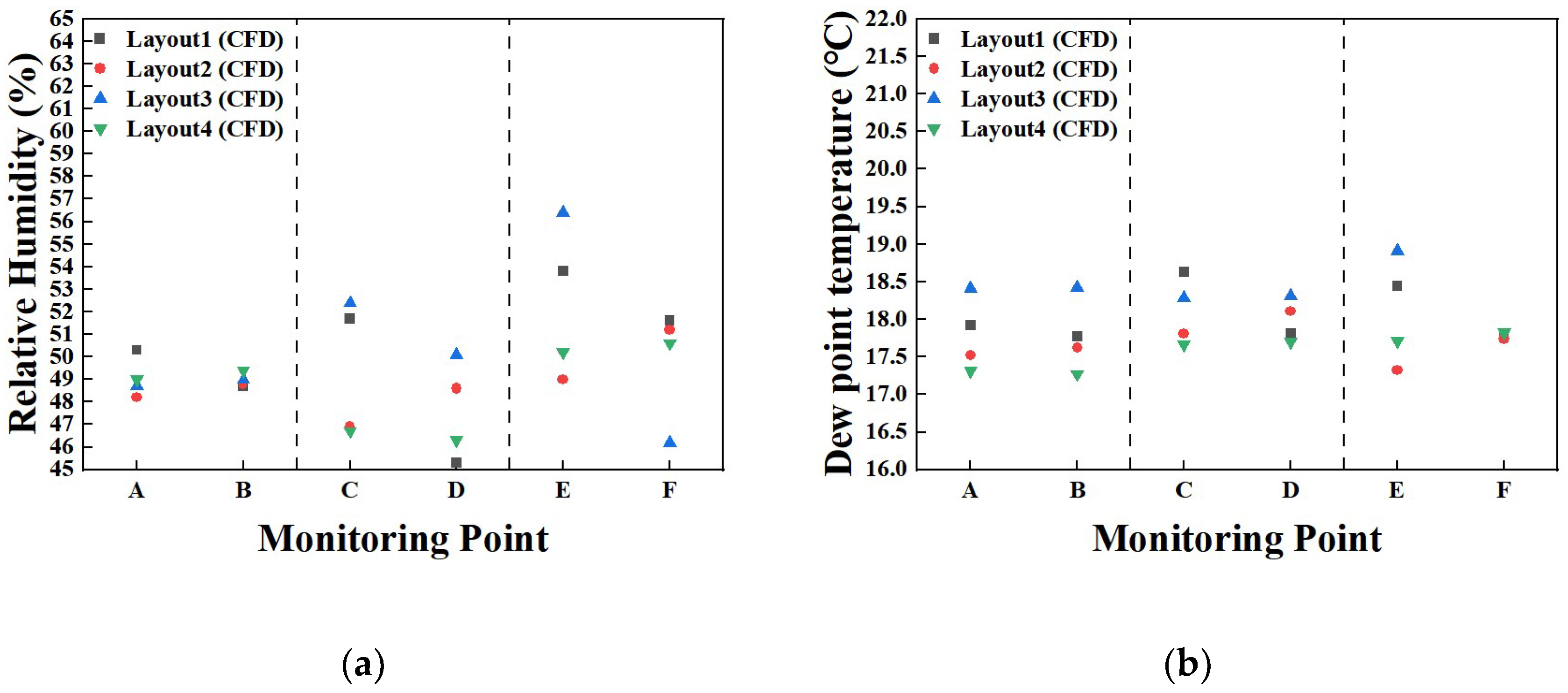
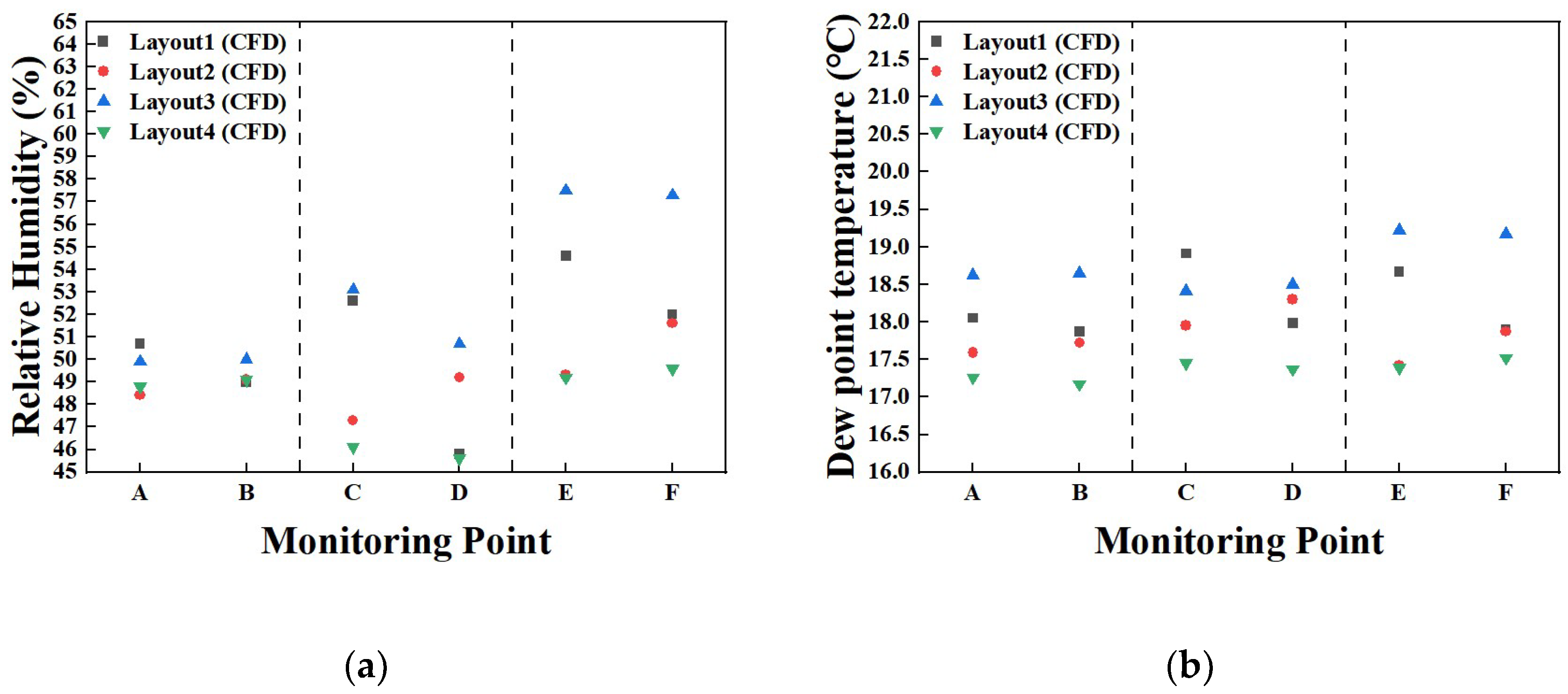
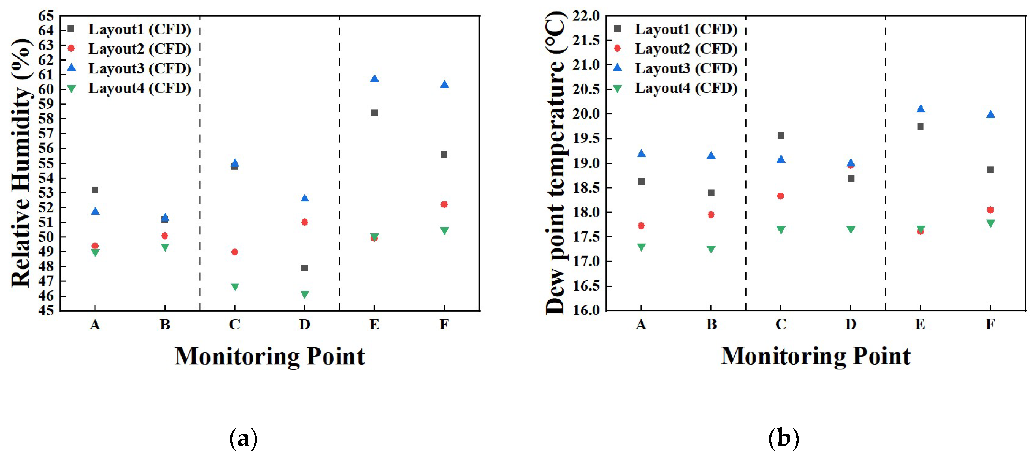
3.3. Simulation Optimization Analysis

3.3.1. Model Optimization

To more accurately reflect the multi-physical field situation inside the cable room, the simulation model was improved to consider the influence of internal structure on the multi-physical field of the cable cabinet. Based on mutual verification experiments, only the internal electric heating wire and heating rod were replaced with three-phase cables and sleeve joints, while the outer cabinet remained unchanged. The geometric structure and dimensions of the simplified cable room model are shown in Figure 2b.

3.3.2. The Impact of Different Humidity Sources on Dehumidification Efficiency

According to [19], the relative humidity at the bottom of the cable trench is mostly maintained in the range of 70–80% during equipment operation. At this point, by changing the humidity of the humidity source, the dehumidification of each layout under different humidity levels can be analyzed. The bottom inlet humidity was set to 75%, 80%, 85%, and 100% as controls. The dehumidification process was examined by comparing the data distributions of different layouts in varying humidity conditions. The relative humidity and dew point temperature under various humidity conditions are illustrated in the following figures.

Firstly, the bottom inlet humidity is 75%, and the data distribution diagram is shown in Figure 8a,b. Layout 4 still has advantages in terms of relative humidity and dew point temperature after steady state, with the lowest relative humidity being 45.1% and the highest only being 49%; the lowest dew point temperature is 17.2 °C, and the highest is only 17.3 °C. Secondly, the bottom inlet humidity is 80%, and the data distribution diagram is shown in Figure 9a,b. Layout 4 still has advantages in terms of relative humidity and dew point temperature after steady state, with the lowest relative humidity being 46.3% and the highest only being 50.6%; the lowest dew point temperature is 17.3 °C, and the highest is only 17.8 °C. Additionally, the bottom inlet humidity was 85%, and the data distribution diagram is shown in Figure 10a,b. Layout 4 still has advantages in both relative humidity and dew point temperature after steady state, with the lowest relative humidity being 45.6% and the highest only being 49.6%; the lowest dew point temperature is 17.2 °C, and the highest is only 17.5 °C. Finally, with the bottom inlet humidity of 100% as the control, the data distribution diagram is shown in Figure 11a,b. Layout 4 has more advantages in both relative humidity and dew point temperature after steady state, with the lowest relative humidity of 46.2% and the highest only 50.5%; the lowest dew point temperature is 17.3 °C, and the highest is only 17.8 °C

In summary, after model optimization, even when the humidity of the humidity source is different, the overall dehumidification of each layout has a similar trend as the previous experiments and simulations before optimization. Layouts 2 and 4 are better than Layout 1, while Layout 3 has the worst effect; Layout 4 has the best dehumidification overall compared to other layouts when the humidity of the humidity source is different. Referring to the condition of 100% relative humidity of the humidity source, under three humidity conditions of 75% and 85%, after Layout 4 reaches steady state, the relative humidity at the measuring point can be reduced by up to 10.6%, reaching as low as 45.1%; the dew point temperature decreased by 2.61 °C, dropping to 17.2 °C. Under different humidity conditions, the maximum difference between the maximum relative humidity values at each measuring point is only 1%, and the maximum difference between the minimum values is only 1.6%; the maximum difference between the maximum dew point temperatures is only 0.1 °C, and the maximum difference between the minimum values is only 0.5 °C, indicating that the dehumidification of Layout 4 is sufficiently stable.

3.3.3. The Impact of Pipeline Layout on the Flow Field of Cable Chambers

A flow field analysis was conducted on the original pipeline layout and the optimal typical interface at Y = 50 mm, and the coordinates on the map represent the X and Z directions of the cable room. The central cavity is a cable hole with a diameter of 110 mm, and it is solid in the positive Y direction. At this point, the three separate cables are wrapped in insulated sleeves and there is no significant change in surface temperature. The negative Y direction leads to the exterior of the cable room, with a sleeve diameter of 100 mm. The humidity supply inlet is a circular ring with an inner diameter of 100 mm and an outer diameter of 110 mm, designed to simulate the pores of the cable hole. By comparing the temperature distribution, relative humidity distribution, and velocity distribution cloud maps of typical cross-sections between Layout 1 and Layout 4 are obtained, as shown in Figure 12 and Figure 13. Comparing the temperature distribution cloud maps in Figure 12a and Figure 13a, on a typical cross-section, the overall temperature of Layout 1 is lower at 301 K, while the local temperature in the upper left corner is slightly higher at 302 K; Layout 4 has an overall temperature of 302 K, with a more uniform distribution. Comparing the temperature distribution cloud maps in Figure 12b and Figure 13b, on a typical cross-section, the overall relative humidity of Layout 1 is above 60%, with higher humidity in the central area near the cable trench; The overall relative humidity of Layout 4 is above 50%, and the fluctuation area near the cable trench is smaller. Comparing the temperature distribution cloud maps in Figure 12c and Figure 13c, on a typical cross-section, Layout 1 has a larger range of velocity fluctuations, with velocities varying around 0.3 m/s in the middle, upper right corner, lower right corner, and directly below; the velocity distribution of Layout 4 is more uniform, with only the middle part and the lower part having a speed close to 0.3 m/s, while there is little change in other parts.

Overall, the flow field distribution in Layout 4 is more stable compared to Layout 1, which affirms the positive significance of optimizing the pipeline layout.

4. Conclusions

In conclusion, a dehumidifier applied to a 10 kV AC outdoor box-type switchgear is studied, which uses dry air for internal circulation. The temperature, humidity, and flow field of the cable compartment inside the switchgear are simulated through CFD-EMAG coupling, and the dehumidification is analyzed through experimental verification with a self-made cable room. Based on the simulation results of the cable room’s humidity, temperature, and velocity fields, optimization measures are proposed to achieve better dehumidification and anti-condensation of RMUs.

Following are some conclusions that can be drawn:

(1)

Based on mutual verification between simulation and experiment, the maximum relative errors of temperature, relative humidity, and velocity at the six monitoring points set in all layout experiments and simulations are only 3.61%, 7.14%, and 7.14%. Meanwhile, the average temperature relative error between experiment and simulation is 2.7% in the electric heating wire, and the errors are both within an acceptable range.

(2)

Based on mutual verification of experimental and simulation results, after optimizing the model, the overall dehumidification has the same trend. Layout 2 and Layout 4 have better dehumidification compared to the original layout. Layout 4 is the optimal layout. After reaching a steady state, compared with other layouts, the relative humidity of the corresponding measurement points is reduced by up to 10.6% with a minimum relative humidity of 45.1%; the dew point temperature can be reduced by up to 2.61 °C, with a minimum dew point temperature of 17.2 °C.

(3)

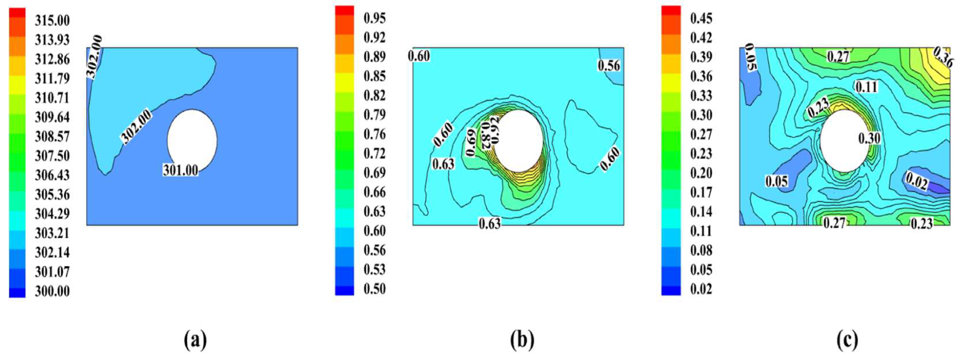
The new layout has a more uniform flow distribution compared to the original layout, with an overall temperature of around 301 K and a relative humidity of 50% on typical cross-sections. The overall distribution of flow velocity is also more uniform, with a maximum of no more than 0.3 m/s. Based on the above experiments and simulations, optimized dehumidification methods and measures have been proposed, providing support for their safe operation. However, this study is mainly based on the experimental environment of 28 °C and 50% humidity, which has certain limitations, and the bidirectional coupling of electric-thermal needs to be further considered. In the future, further research will be conducted based on more environmental conditions, providing more references for the prevention of condensation in RMU.

References

1. Cheng, H.; Zhang, X.; Tang, J.; Xiao, S. The application of fluorescent optical fiber in partial discharge detection of Ring Main Unit. Measurement 2021, 174, 108979. [Google Scholar] [CrossRef]
2. Bharat Heavy Electricals Limited. Handbook of Switchgears; McGraw-Hill: New Delphi, India, 2006. [Google Scholar]
3. Jiang, T.; Sun, W. Analysis and solution of dewing problems for the looped-network switchgear. Rural. Electr. 2011, 19, 28. [Google Scholar]
4. Xu, X.Y. 110–500 kV analysis of composite insulator flashover on transmission line and countermeasure of China. China Power 2000, 33, 54–56. [Google Scholar]
5. Zeng, W. Study and practice of anti-condensation technology for high-voltage switchgear. Metall. Power 2016, 32, 49–50. [Google Scholar]
6. Lin, F. Indoor dewing phenomenon and strategy in metal-enclosed switchgear. Premiere 2017, 28, 196. [Google Scholar]
7. Pan, Q.Z.; Yang, F.; Tang, X.L.; Yang, L.; Liu, S.L. Simulation environment design for the investigation of damping and dewing mechanisms in the 12 kV high-voltage switchgear. E3S Web Conf. 2018, 53, 03001. [Google Scholar] [CrossRef]
8. Geng, J.H.; Guo, Q.; Xu, Z.; Liu, R. Research of outdoor equipment condensation development process based on improved morphology and optimization of condensation prevention measures. Sci. Technol. Eng. 2016, 22, 213–218. [Google Scholar]
9. Yue, X.F. Discussion about the heating and dehumidification system in 12 kV switchgear. High Volt. Appar. 2002, 38, 57–58. [Google Scholar]
10. Wang, Y.; Ding, Y.; Li, W. Humidity control of RMU based on COMSOL simulation analysis. Electr. Power 2020, 53, 206–213. [Google Scholar] [CrossRef]
11. Bedkowski, M.; Smolka, J.; Banasiak, K.; Bulinski, Z.; Nowak, A.; Tomanek, T.; Adam, W. Coupled numerical modelling of power loss generation in busbar system of low-voltage switchgear. Int. J. Therm. Sci. 2014, 82, 122–129. [Google Scholar] [CrossRef]
12. Chen, R.; Yan, X.; Yan, W.; Zhang, C.; Liu, W.; Yang, K. Numerical simulation on condensation phenomenon in the switch cabinet. Resour. Sav. Environ. Prot. 2015, 5, 21–23. [Google Scholar] [CrossRef]
13. Zhang, W.; Yan, Z.; Wang, Y. Anti-condensation method for outdoor RMU based on finite element analysis. High Volt. Appar. 2017, 53, 101–106, 113. [Google Scholar] [CrossRef]
14. Wu, Y.; Ruan, J.; Li, P. Optimum simulation of thermal field for switchgear. Electr. Mach. Control. 2020, 24, 1. [Google Scholar] [CrossRef]
15. Pan, Q.Z.; Yang, F.; Yang, Z. Discussion on mechanism of the dampness and dewing inside 12 kV high-voltage switchgear and its key control techniques. Power Syst. Prot. Control. 2019, 47, 160–172. [Google Scholar] [CrossRef]
16. Zheng, X.; Hu, F.; Wang, Y.; Zhang, H.; You, S.; Shi, R.; Shi, K. Optimization on airflow distribution for anti-condensation of high-voltage switchgear using CFD method. Case Stud. Therm. Eng. 2021, 28, 101479. [Google Scholar] [CrossRef]
17. Pan, M.L. Research on Influence Law of Force on the Bushing Affected by Cable Bending in 10 kV RMU. Master’s Thesis, Three Gorges University, Yichang, China, 2018. [Google Scholar]
18. Li, Z.W. Temperature Field Modeling and Thermal Analysis of Medium Voltage Switchgear Based on ANSYS. Master’s Thesis, Shanghai University of Engineering Science, Shanghai, China, 2020. [Google Scholar]
19. Luo, W.Z.; Xiong, X.X.; Chen, C.; Lin, P. Research on Dehumidification Scheme of Cable Treanch in 35 kV Switchgear Room. Electr. Eng. 2022, 573, 145–147. [Google Scholar] [CrossRef]
Figure 1. The flowchart of research.
Applsci 14 01602 g001
Figure 2. (a) Geometric structure and dimensions of cable room model with electric heating wire, (b) geometric structure and dimensions of simulation model with cables, (c) schematic diagram of the main grid of the cable room and (d) XYZ coordinates and reference points of the main monitoring points.
Applsci 14 01602 g002
Figure 3. (a) Ventilating pipes layout 1 and 2; (b) ventilating pipes layout 3 and 4.
Applsci 14 01602 g003
Figure 4. (a) The velocity variation trend of different grid monitoring points in the cable room model with electric heat wire of the verification experiment; (b) the velocity variation trend of different grid monitoring points in the cable room model with cables.
Applsci 14 01602 g004
Figure 5. (a) Diagram of the initial experimental cable room and related experimental equipment; (b) diagram of a 12 L drying dehumidifier used in the experiment in front of the ventilating pipe.
Applsci 14 01602 g005
Figure 6. (a) Diagram of the internal structure and measurement points of the experimental cable room; (b) diagram of the ventilation duct and corresponding measurement points in the improved experimental cable room.
Applsci 14 01602 g006
Figure 7. (a) Distribution of monitoring points’ relative humidity data for each layout in the experiment and simulation; (b) distribution of monitoring points’ dew point temperature data for each layout in the experiment and simulation.
Applsci 14 01602 g007
Figure 8. (a) Distribution of relative humidity data at 75% bottom inlet humidity; (b) distribution of dew point temperature data at 75% bottom inlet humidity.
Applsci 14 01602 g008
Figure 9. (a) Distribution of relative humidity data at 80% bottom inlet humidity; (b) distribution of dew point temperature data at 80% bottom inlet humidity.
Applsci 14 01602 g009
Figure 10. (a) Distribution of relative humidity data at 85% bottom inlet humidity; (b) distribution of dew point temperature data at 85% bottom inlet humidity.
Applsci 14 01602 g010
Figure 11. (a) Distribution of relative humidity data at 100% source humidity; (b) distribution of dew point temperature data at 100% bottom inlet humidity.
Applsci 14 01602 g011
Figure 12. (a) Temperature (K), (b) relative humidity, and (c) velocity (m/s) fields of layout 1 at Y = 50 mm cross-section when the humidity source is 100%.
Applsci 14 01602 g012
Figure 13. (a) Temperature (K), (b) relative humidity, and (c) velocity (m/s) fields of layout 4 at Y = 50 mm cross-section when the humidity source is 100%.
Applsci 14 01602 g013