Numerical Investigation of a Novel Grinding Device for the One-Pot Production of Ferromagnetic Nanoparticles

Featured Application

The proposed procedure allows for the simple, efficient, and sustainable production of magnetic nanoparticles, which can be readily used in one-pot purification processes.

Abstract

The use of nanoparticles (NPs) in industrial applications is consistently increasing given their peculiar properties compared to bulk precursor materials. As a result, there is a growing need to develop alternative technical strategies for the synthesis of such NPs using processes that are not only environmentally friendly but also easy and inexpensive to implement on an industrial scale. In this regard, a novel approach has recently been proposed for the safe and sustainable production of metal NPs directly from a bulky solid by magnetically driven low-energy wet milling, which overcomes the limits of applicability to ferromagnetic materials through a unique device configuration. In the present contribution, the understanding of this alternative configuration is deepened by computational investigation. Discrete Element Method (DEM) simulations were used to model the dynamics of the system, highlighting the role of the various parameters involved in the setup and operation of the process. The collisions between grinding and primary particles are analyzed in terms of frequency, impact angle, and energy. Comparing the results with the standard device configuration, the general trend is preserved, though collisions at higher impact angle and energy are also detected.

1. Introduction

Nanoparticles (NPs) and nanostructured materials are now playing a central role in the global scientific landscape due to their versatility in a wide variety of technical applications [1]. Their use relies on features such as enhanced chemical reactivity resulting from the high surface-to-volume ratio [2,3]. Examples include industrial [4], medical [5,6], and environmental [7,8] applications. In addition, the combination of different nanomaterials, such as metallic nanoparticles and carbon nanostructures, makes it possible to produce new hybrid composites with interesting properties that combine the advantages of both [9].

The synthesis procedure, selected depending on the specific compound and its application, can basically follow one of two opposite strategies, namely bottom-up and top-down, the former being more widespread [10]. Indeed, it is easier to monitor the synthesis by progressive aggregation around seeds than during disaggregation, but very often these methods require the use of various chemicals that can be harmful to humans and the environment [11,12].

In response to increasingly stringent constraints on the environmental sustainability of products and processes [13], research is constantly focused on the development of new approaches and procedures generally known as ‘green nanotechnologies’ [14,15]. Among them, top-down synthesis methods, which involve the physical comminution of macroscopic elements or compounds without any chemical reaction, are attracting increasing interest [16].

Several disaggregation techniques have been proposed [17], including the use of grinding media such as beads [18,19]. However, a known shortcoming of these methods is the poor control over the particle size distribution that requires the adoption of specific strategies [20], including the use of stabilizing agents to prevent the tendency of the produced NPs to reaggregate [21,22].

A novel custom device under development for the top-down physical synthesis of NPs via wet mechanical refining is described in Reverberi et al. [10]. Such a device offers several advantages in terms of safety, convenience, and environmental friendliness, since it allows NPs to be produced in a one-pot operation, i.e., directly as a suspended phase in the process solvent and directly from a bulky solid such as millimeter-sized metal spheres. Due to the establishment of special operating conditions, it has been observed that this configuration allows the production of NPs with a size reduction factor of up to 1/10⁵ compared to the precursor beads. This makes it possible to overcome the well-known rule of thumb that sets the limit of the reduction factor for this type of processes at 1/1000 [10].

To expand the application potential of the discussed approach while preserving its advantages, an alternative configuration of the device has also been developed and tested for the production of Ag glyconanoparticles with a narrow size distribution in the range 10–20 nm [16]. In this new setup, the stirring is performed by an impeller that is driven by a magnetic bar kept outside the fluid containing the precursor beads. As a result, in the case of ferromagnetic NPs, particle magnetization and consequent aggregation are avoided, in contrast to the original configuration, thus favoring a more stable and homogeneous dispersion. The complete confinement of the impeller shaft inside the vessel enables operation under pressure and/or with volatile solvents. In addition, it is also suitable for one-pot purification processes, where the NPs are used as soon as they are produced, with obvious advantages in terms of safety, cost, and the environment.

Considering the same synthesis of silver NPs previously studied in the standard apparatus [23], a first attempt to investigate the new configuration by means of numerical simulations was made in Trofa et al. [24].

The aim of the present work is to deepen the analysis by considering additional operating conditions, including different stirring speeds and loading configurations. The process is modeled through the Discrete Element Method (DEM), which can reproduce the movement and collisions of the precursor and grinding beads. Although no direct information about the produced NPs can be obtained from DEM simulations, such an approach provides access to key system features, such as impact frequency, energy, and angle. This makes it possible to understand how changes in the experimental setup affect the dynamics of the system and, ultimately, the efficiency of the abrasion process underlying the generation of NPs.

2. Materials and Methods

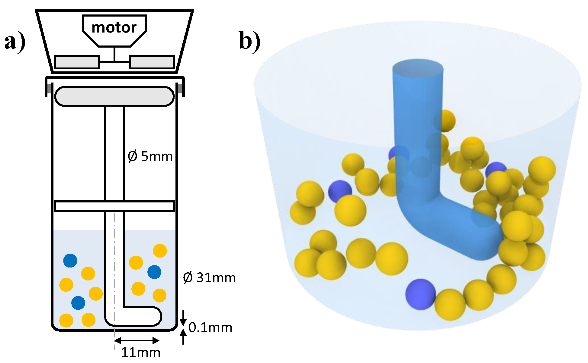
2.1. Experimental Setup

The scheme of the novel custom-made wet milling device is reported in Figure 1a. As in [24], the main components are the following:

• A cylindrical container (height 120 mm, internal diameter 31 mm, glass);
• A cylindrical magnetic bar (hemispherical ends, length 30 mm, diameter 5 mm, PTFE coating);
• An L-bent rotating shaft (hemispherical end, diameter 5 mm, L-arm length 11 mm, glass);
• 4 metal precursor beads (diameter 3 mm, Ag 99.9% (American Elements, Los Angeles, CA, USA));
• 40 grinding beads (diameter 3 mm, ZrO₂ 95%, Y₂O₃ 5% (MSE Supplies, Tucson, AZ, USA), materials known for their high surface hardness and anti-scratch properties).

The position of the magnetic bar represents the fundamental innovation compared to previous configuration [23]. Since the bar is kept outside the liquid containing the beads, this apparatus is known as outer-bar wet miller (OWM) as opposed to the original inner-bar wet miller (IWM) [16]. The aforementioned magnetic bar drives an L-bent glass shaft, coated at the bottom with PTFE to minimize attrition, which keeps the grinding and precursor beads in motion. The rotation causes the beads to collide and the metal precursor to wear off, releasing NPs. A detailed description of the aforementioned experimental setup is available elsewhere [16].

Note that when the torque applied by the magnetic drive is overcome by the resisting torque of the beads, the process stops abruptly. This occurs, for example, when the number of beads in the vessel exceeds a certain critical threshold, which is determined by system geometric parameters such as bead size, container shape, and impeller shape and position. In this regard, the OWM has a lower tendency to jam because it is able to exploit all of the available torque with a magnetic bar that rotates parallel to the motor. Conversely, the IWM wastes part of the torque due to the inclined magnetic bar. This advantage makes the OWM configuration more suitable for autogenous grinding, i.e., when only metal precursor beads are used (which generally have a higher density and therefore a higher inertia). On the other hand, to prevent shaft blockage and breakage, the OWM requires careful design and control of the impeller. This constraint adds complexity to the design but is more than compensated by the benefits it provides, resulting in a much higher hourly output of metallic NPs [16].

Most importantly, the ability to abrade ferromagnetic materials to produce the corresponding NPs is a unique advantage of the OWM setup. Indeed, the IWM is unable to achieve this result since the precursor beads and produced NPs would be attracted by the magnetic field generated by both the stirring bar and the external motor, resulting in magnetic-induced NP aggregation and a severe reduction in grinding efficiency.

2.2. Numerical Setup

The computational domain used to perform the numerical study is schematically reported in Figure 1b. ZrO₂ grinding beads are yellow, and Ag precursor beads are blue. The stirring movement is imposed by the counterclockwise rotation around the container axis of the L-bent glass shaft.

The motion and collisions of the beads in the grinding system are modeled through the Discrete Element Method [25]. For each particle i, the translational ${\mathit{u}}_i$ and angular ${\mathit{\omega }}_i$ velocities are computed from Euler’s laws of motion (i.e., the force and torque equations for rigid-body motion):

$$m_i\frac{d{\mathit{u}}_i}{dt}=\sum _j{\mathit{F}}_{\mathrm{c}}+m_i\mathit{g}{I}_i\frac{d{\mathit{\omega }}_i}{dt}=\sum _j{\mathit{T}}_{\mathrm{c}}$$

(1)

where $m_i$ and $I_i$ are the particle mass and moment of inertia and $\mathit{g}$ is the gravity vector. The force ${\mathit{F}}_{\mathrm{c}}$ and the torque ${\mathit{T}}_{\mathrm{c}}$ are due to the j contacts with other particles or the container and are calculated through the Hertz–Mindlin model [23]:

$$\begin{array}{c}{\mathit{F}}_{\mathrm{c}}=F_{\mathrm{c},\mathrm{n}}\mathit{n}+F_{\mathrm{c},\mathrm{t}}\mathit{t}=\left(k_{\mathrm{n}}{\delta }_{\mathrm{n}}+{\gamma }_{\mathrm{n}}\frac{d{\delta }_{\mathrm{n}}}{dt}\right)\mathit{n}-\left(k_{\mathrm{t}}{\delta }_{\mathrm{t}}+{\gamma }_{\mathrm{t}}\frac{d{\delta }_{\mathrm{t}}}{dt}\right)\mathit{t}\end{array}$$

(2)

$$\begin{array}{c}{\mathit{T}}_{\mathrm{c}}=-r_i{F}_{\mathrm{c},\mathrm{t}}\mathit{n}\times \mathit{t}\end{array}$$

(3)

In the previous equations, $\mathit{n}$ is the unit normal vector to the contact plane (pointing from j to i), and $\mathit{t}$ is the direction of tangential motion between the contacting surfaces. The symbols ${\delta }_{\mathrm{n}}$ and ${\delta }_{\mathrm{t}}$ denote the normal and tangential overlaps, $k_{\mathrm{n}}$ and $k_{\mathrm{t}}$ are the normal and tangential stiffnesses, and ${\gamma }_{\mathrm{n}}$ and ${\gamma }_{\mathrm{t}}$ are the normal and tangential damping coefficients. The tangential component of the contact force is limited by the Coulomb law of sliding friction $\left|F_{\mathrm{c},\mathrm{t}}\right|\le {\mu }_{\mathrm{F}}\left|F_{\mathrm{c},\mathrm{n}}\right|$, with ${\mu }_{\mathrm{F}}$ the sliding friction coefficient. These quantities depend on particle dimensions and material properties such as density, Young’s modulus, and Poisson ratio. The values employed in the present study have been taken from the literature and are listed in

Table 1. Model parameters and material properties (see [27] for zirconia and glass, [28] for silver, and [29] for PTFE). Reprinted with permission from Ref. [24], 2023, AIDIC Servizi S.r.l.

	Zirconia, ZrO2	Silver, Ag	Glass	PTFE
Density [kg/m3]	6067	10,490	2510	2200
Young’s Modulus [GPa]	210.0	82.0	70.0	0.50
Poisson ratio	0.31	0.36	0.24	0.46
Coefficient of restitution	0.92	0.80	0.99	0.80
Coefficient of friction	0.15	0.55	0.27	0.08

. Note that the values of the restitution and friction coefficients are subject to some uncertainty, since they depend on several parameters (e.g., temperature, contact geometry, and applied force) specific to the system they were measured with [26]. In addition, the adopted model assumes a fixed restitution coefficient (independent of the impact velocity) and considers the average value of the friction coefficients for the material pairs.

The particle trajectory is finally obtained by integrating the following kinematic equations for position ${\mathit{x}}_i$ and orientation ${\mathit{\theta }}_i$, starting from the initial values ${\mathit{u}}_{i,0}={\mathit{\theta }}_{i,0}={\mathit{\omega }}_{i,0}=\mathbf{0}$ and a random non-overlapping position inside the domain:

$$\frac{d{\mathit{x}}_i}{dt}={\mathit{u}}_i\frac{d{\mathit{\theta }}_i}{dt}={\mathit{\omega }}_i$$

(4)

More details about the DEM model used here and the related parameters can be found in [23].

The analysis of the collisions requires examination of the relative velocity between the contacting particle surfaces ${\mathit{v}}_{\mathrm{c}}={\mathit{v}}_i-{\mathit{v}}_j$, where the velocity of the $i-$th particle surface ${\mathit{v}}_i={\mathit{u}}_i+{\mathit{\omega }}_i\times {\mathit{r}}_i$ is computed from the quantities in Equation (4) and the position vector from the particle center to the contact point ${\mathit{r}}_i$. From the relative velocity at the beginning of the contact (which has normal and tangential components $v_{\mathrm{c},\mathrm{n}}$ and $v_{\mathrm{c},\mathrm{t}}$), it is possible to compute the impact kinetic energy $k{e}_{\mathrm{r}}$ and the impact angle ${\theta }_{\mathrm{impact}}$:

$$\begin{array}{c}k{e}_{\mathrm{r}}=\frac{1}{2}{\mathit{v}}_{\mathrm{c}}^{\mathrm{T}}·\mathit{M}·{\mathit{v}}_{\mathrm{c}}=\frac{1}{2}\left(v_{\mathrm{c},\mathrm{t}}{v}_{\mathrm{c},\mathrm{n}}\right)·{\left(\frac{1}{m_i}+\frac{1}{m_j}\right)}^{-1}\left(\begin{array}{cc}2/7& 0\\ 0& 1\end{array}\right)·\left(\genfrac{}{}{0pt}{}{v_{\mathrm{c},\mathrm{t}}}{v_{\mathrm{c},\mathrm{n}}}\right)\end{array}$$

(5)

$$\begin{array}{c}{\theta }_{\mathrm{impact}}=arctan\left(\frac{v_{\mathrm{c},\mathrm{n}}}{v_{\mathrm{c},\mathrm{t}}}\right)\end{array}$$

(6)

where $\mathit{M}$ is the inertia matrix of the system of two spherical particles [30]. Such matrix is symmetric, positive definite, and contains the coefficient 2/7 connected to the gyration radius of spheres.

The simulations are initialized by randomly placing the beads in the vessel and allowing them to settle for 0.5 s, reaching a pseudo-steady-state condition. The contact sampling is then performed in the following 5 s, corresponding to 50 complete revolutions of the impeller at 600 rpm. A customized procedure, by monitoring the changes in particle–particle and particle–wall contacts at every time step, allows the identification of new contacts (i.e., collisions) and detachments and consequently collision frequency and duration [31].

The numerical integration is performed with a time step of 10⁻⁷ s, sufficiently smaller than the actual collision time (whose scale is given by Rayleigh and Hertz times) [25]. This value ensures the stability of the numerical simulations and a proper resolution of the impact dynamics. To ensure the statistical invariance of the insertion method, the results reported in the following section are obtained by averaging over 6 simulations with distinct random seeds, which determine the particle starting positioning in the computational domain.

To implement and execute the code, the open-source software LIGGGHTS^® 3.8.0 was used (further information can be found in [32]).

3. Results

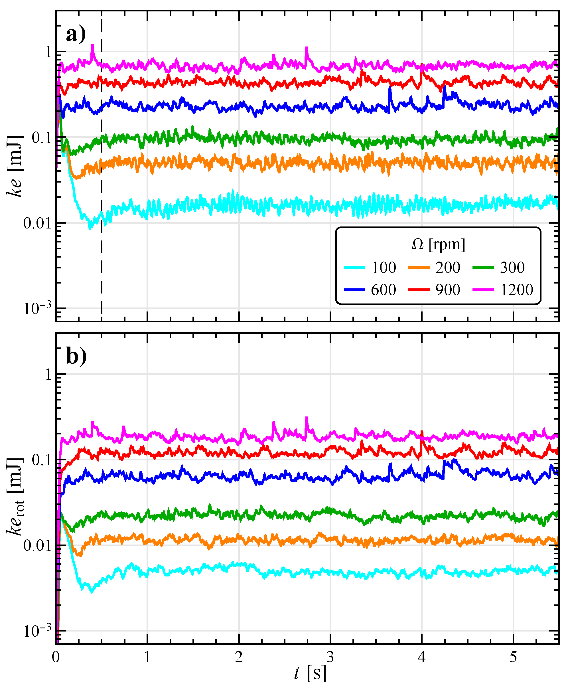
3.1. Preliminary Stability Analysis

Figure 2 shows the temporal trend of the total translational and rotational kinetic energy of all the particles in the system ($ke=0.5\sum m_i{\mathit{u}}_i^2$ and $k{e}_{\mathrm{rot}}=0.5\sum I_i{\mathit{\omega }}_i^2$) at different stirring velocities Ω. As explained in the previous section, each curve represents the average over six simulations with different random seeds. Moreover, the fast fluctuations have been filtered with a moving average of radius 5.

In all the cases, it is possible to distinguish a fast initial transient and a pseudo-steady-state regime. The former is connected to the initialization procedure and lasts less than 0.5 s (dashed gray line in Figure 2a). The latter is apparent from a nearly constant value proportional to the stirring velocity (${ke}_{\mathrm{steady}}\propto {\mathsf{\Omega }}^{1.5}$).

Comparing both kinetic energies with the related values of the corresponding IWM configuration [23], an increase by a factor of around 2 was found, ascribable to the longer stirring arm and consequent higher tip speed.

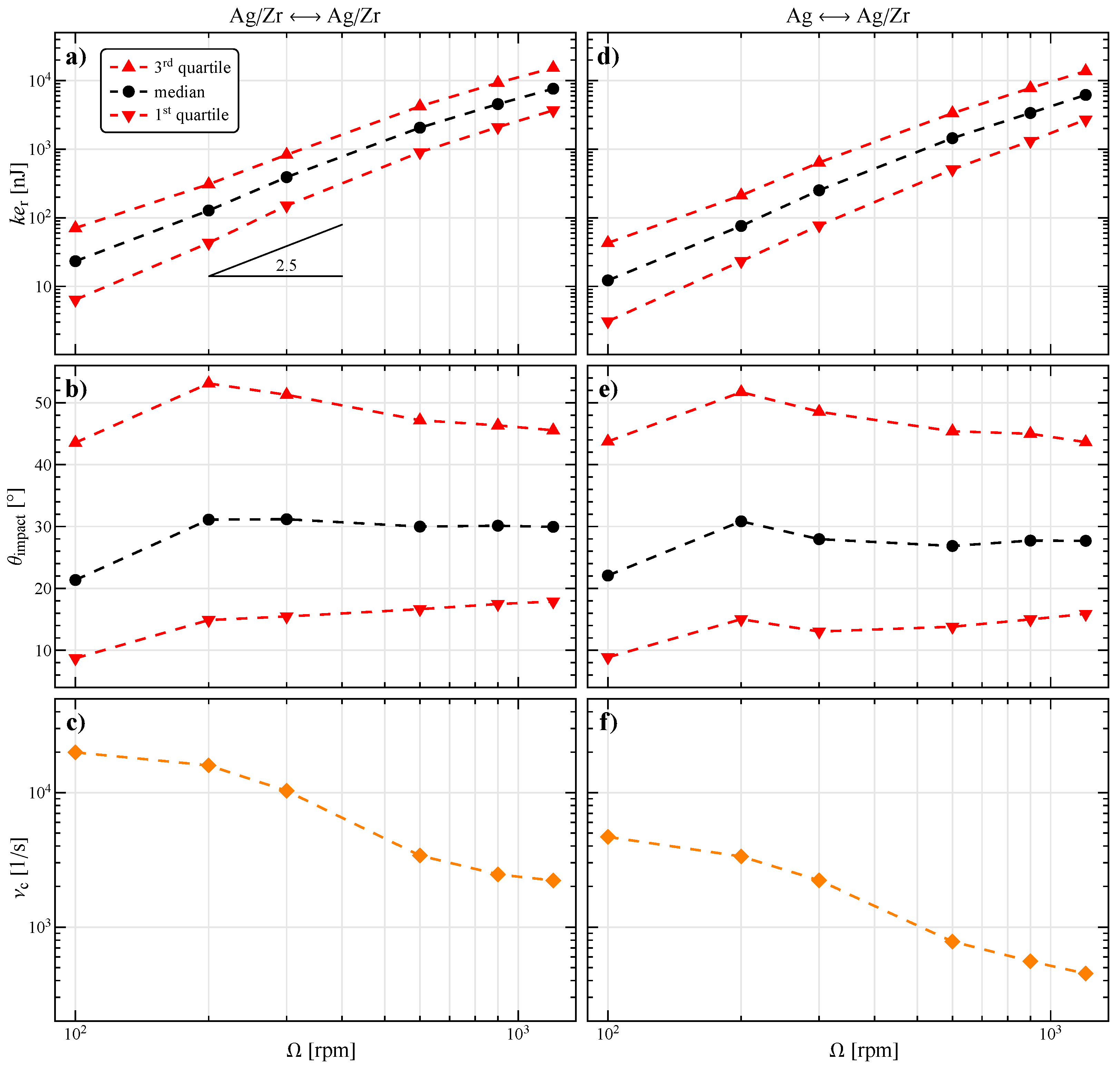
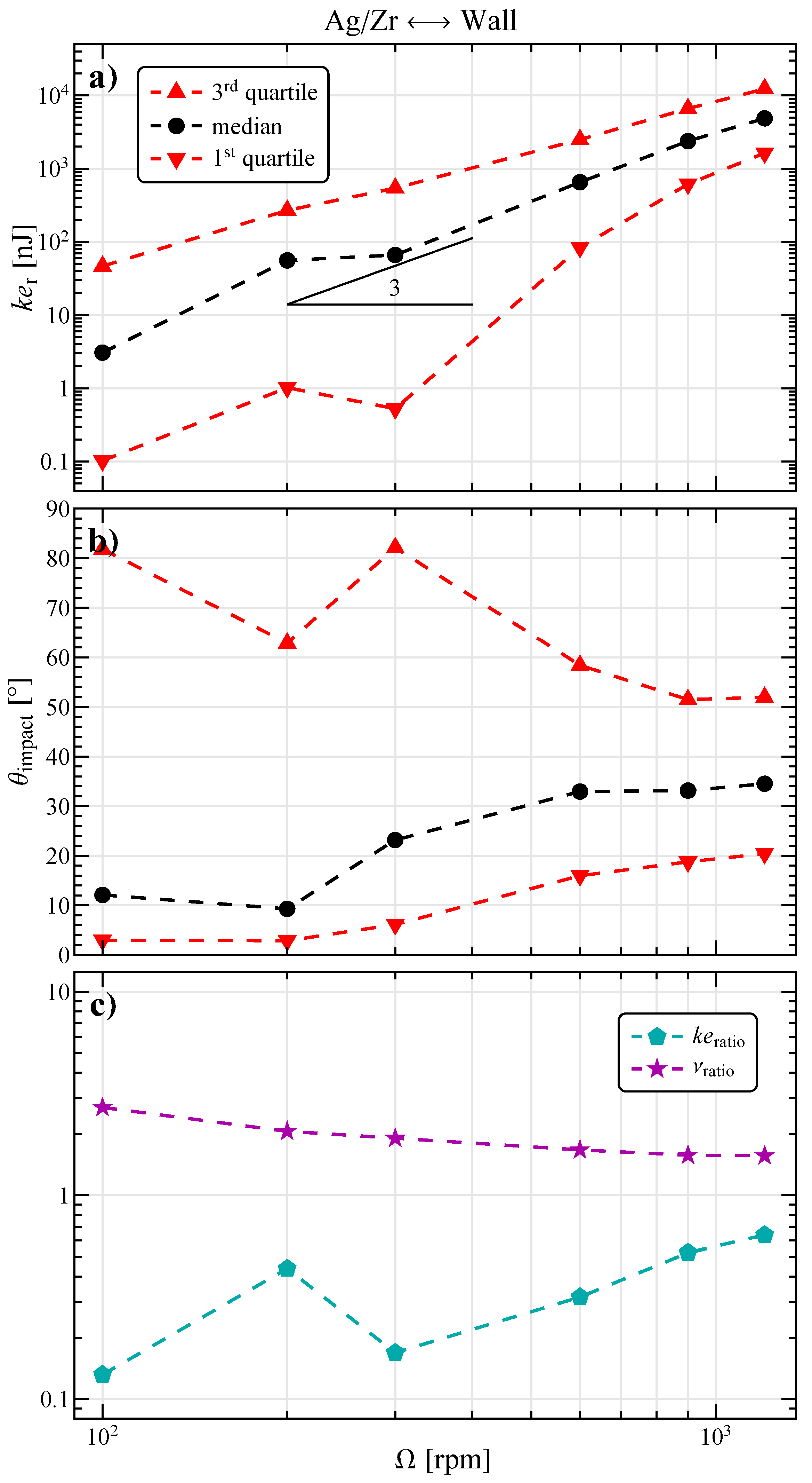
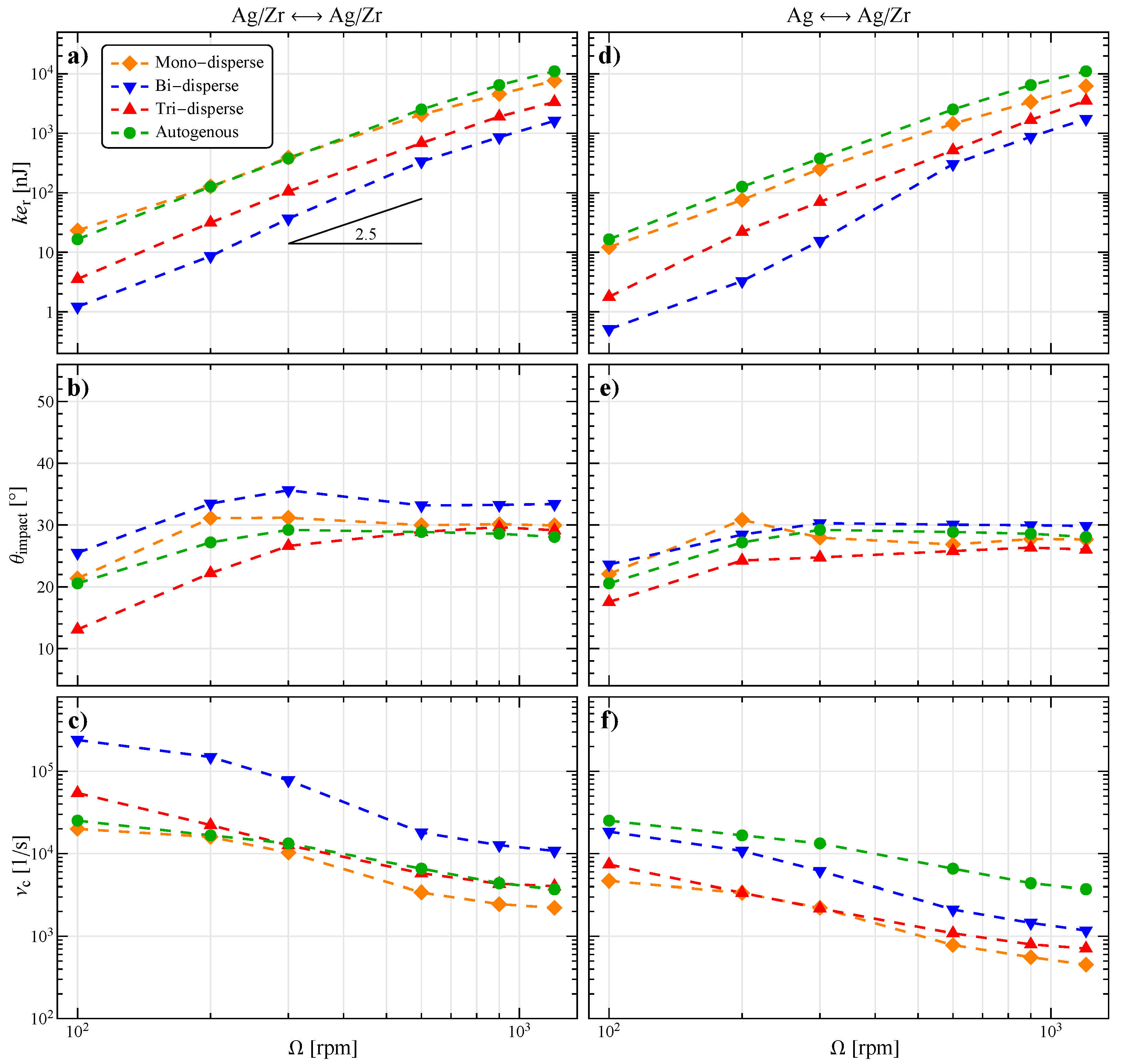
3.2. General Characterization of Collisions

The milling process involves thousands of collisions per second, with a variety of impact dynamics. To better understand the general behavior of the system, it is useful to look at the descriptors of the distributions that characterize the variables of interest. In particular, considering particle–particle collisions, the quartiles of the distribution of impact kinetic energy $k{e}_{\mathrm{r}}$ and impact angle ${\theta }_{\mathrm{impact}}$ are shown in the first two rows of Figure 3, whereas the last row contains the average collision frequency ${\nu }_{\mathrm{c}}$. While the left-hand column (panels a, b, and c) refers to the impacts between all the beads (either Ag or ZrO₂), the right-hand column (panels d, e, and f) is for those involving at least one Ag particle.

The impact kinetic energy, which spans different orders of magnitude, as one can expect, increases with the stirring velocity. Interestingly, the trend of the distribution median can be fairly described by a power-law with an exponent around 2.5 (i.e., $k{e}_{\mathrm{r}}\propto {\mathsf{\Omega }}^{2.5}$).

The median of the impact angle, excluding the 100 rpm case, has an almost constant value of 30°, revealing a prevalent tangential component in the collision velocity. The interquartile range is also almost constant and roughly spans 30°. These results are positive for the production of NPs, since ductile materials (such as Ag) have been shown to exhibit maximum abrasion efficiency at low impact angles [33,34,35].

At low Ω, all the particles are confined on the bottom of the vessel and present a quasi-rigid collective motion determined by the impeller. At higher Ω, the distance among the particles increases, and the collisions become more rare, thus lowering the impact frequency (see Figure 3c).

Similar trends can be encountered by looking at the right-hand column of Figure 3, which illustrates the collisions of the Ag particles (i.e., the NP precursors). Despite the greater density of silver with respect to zirconia, the impact kinetic energy is reduced by a factor of around 2 at 100 rpm and 1.2 at 1200 rpm. Therefore, the impact velocity must be lower. Since Ag only accounts for 4 out of the total 44 particles, one would expect a corresponding reduction in the impact frequency, but this is not the case, as only a reduction to 1/5 was found at all stirring speeds. This is probably because each particle has a different collision frequency, with the Ag ones having higher values, and the curve shown in the figure just represents the total. Notwithstanding such a positive aspect, the decreasing trend of ${\nu }_{\mathrm{c}}$ with Ω remains.

To maximize NP production, it is necessary to balance all the three relevant quantities described above. Notice that, as shown experimentally in the case of IWM [23], there is an optimal operating range for the impact kinetic energy. Indeed, abrasion (i.e., the removal of small surface portions) does not occur below a critical value of $k{e}_{\mathrm{r}}$, and plastic deformations or the production of macroparticles takes place when this is too high. Therefore, since ${\theta }_{\mathrm{impact}}$ is only slightly affected by Ω and it is desirable to maximize ${\nu }_{\mathrm{c}}$, the optimal stirring speed is the minimum that is sufficiently energetic to produce NPs.

Comparing the data in Figure 3 with the corresponding one for the IWM [23], it emerges that the OWM configuration with the same number of particles presents an higher but constant impact angle, an increase in impact kinetic energy of an order of magnitude, and a similar reduction in the impact frequency. Similarly to the total kinetic energy, this difference is probably related to the higher tip speed and reduced confinement.

The collisions between the beads and the container wall are also taken into account, and the corresponding data are reported in Figure 4. The last panel shows the ratio of impact kinetic energy $k{e}_{\mathrm{r},\mathrm{w}}/k{e}_{\mathrm{r},\mathrm{pp}}$ and impact frequency ${\nu }_{\mathrm{c},\mathrm{w}}/{\nu }_{\mathrm{c},\mathrm{pp}}$ between the collision with the wall and those among the beads.

The general trends are similar to those of Figure 3a,b for the collisions among particles; however, here, there is a non-monotonous behavior around 200 rpm. This is likely due to a regime change in the particle motion.

Indeed, at low Ω (i.e., 100 rpm), all the beads remain at the bottom of the vessel and are displaced by the stirring arm in a quasi-rigid collective motion. The friction with the container floor induces rolling and increases the tangential component of collisions, thus determining a low median of ${\theta }_{\mathrm{impact}}$. At the same time, the interquartile range is wide, revealing the presence of almost purely normal collisions, likely those with the vessel lateral wall.

At 200 rpm, the increased centrifugal force pushes the beads from the center to the periphery, where the tangential velocity of rotation around the axis is greater, and some beads start to jump over the impeller. This results in fewer low-energy, high-angle collisions, as evidenced by the shift in the distributions.

As Ω continues to grow (300 rpm and above), the beads are more frequently lifted off the ground by the stirring arm and repopulate the center, the collisions become less tangential, and the median of ${\theta }_{\mathrm{impact}}$ first increases then stabilizes slightly above 30°.

Figure 4c evidences that the collisions with the container wall are more frequent but significantly less energetic than those among the beads. This difference decreases with Ω as the impact velocity with the stationary wall grows more than the one among the beads.

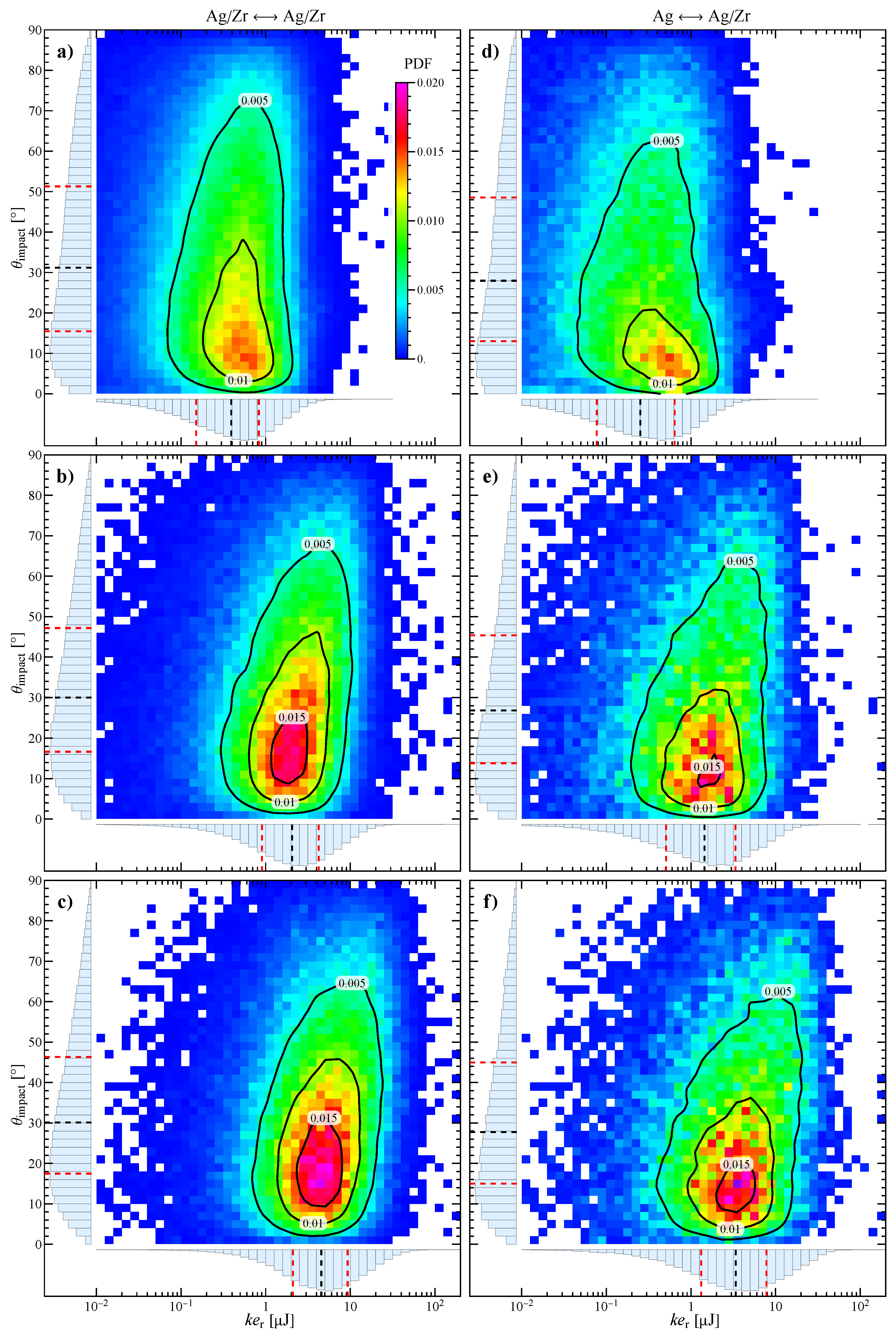
3.3. Detailed Distribution of Collisions

Figure 5 shows the joint probability density function (PDF, with color map and contours) for the impact angle and the logarithm of the impact kinetic energy to further characterize the collisions and identify the optimal operating conditions. The marginal probability density functions and corresponding quartiles (the same as in Figure 3a,b) are also reported on the edges of each map. The joint distribution is built with a binning size of 2° for ${\theta }_{\mathrm{impact}}$ and 0.1 for ${log}_{10}\left(k{e}_{\mathrm{r}}\right)$. Thus, the probability of finding a collision with its parameters in a specific 2D bin (i.e., a ‘pixel’ of the figure) is the value of the bin multiplied by its area, i.e., 0.2. By further multiplying by the impact frequency and the operation time, the total number of collisions with a specific set of parameters is determined. Based on the optimization constraints discussed earlier, the in-depth analysis is limited to the cases of experimental interest with Ω spanning from 300 to 900 rpm.

The joint distributions in Figure 5 are all unimodal, and the most likely collisions have slightly higher kinetic energy and lower impact angle than the corresponding medians (as evident in panel a). At variance with the IWM that presented a negative correlation between ${\theta }_{\mathrm{impact}}$ and $k{e}_{\mathrm{r}}$, these variables are almost uncorrelated at 300 rpm and have a weak positive correlation at higher Ω. In addition, the marginal distribution of ${\theta }_{\mathrm{impact}}$ has an evident positive skewness (with a long tail at high angles). Thus, although most impacts are mainly tangential, some normal ones do occur.

By increasing Ω (from top to bottom in figure) the joint distribution shifts to the right (i.e., the impact kinetic energy increases) and becomes more compact and uniform with respect to the impact angle, as seen in Figure 3.

As concerns the collisions of Ag (right column in Figure 5), the distributions are more scattered due to the lower number of data, marginally more spread for both variables, and slightly shifted at lower $k{e}_{\mathrm{r}}$.

It is possible to determine the optimal operating conditions experimentally (e.g., Ω) to maximize the quality and quantity of NPs. Combining this information with the distributions shown here, the optimization can be related to specific impact conditions (angle and energy) that can then be applied to any given bead mill system.

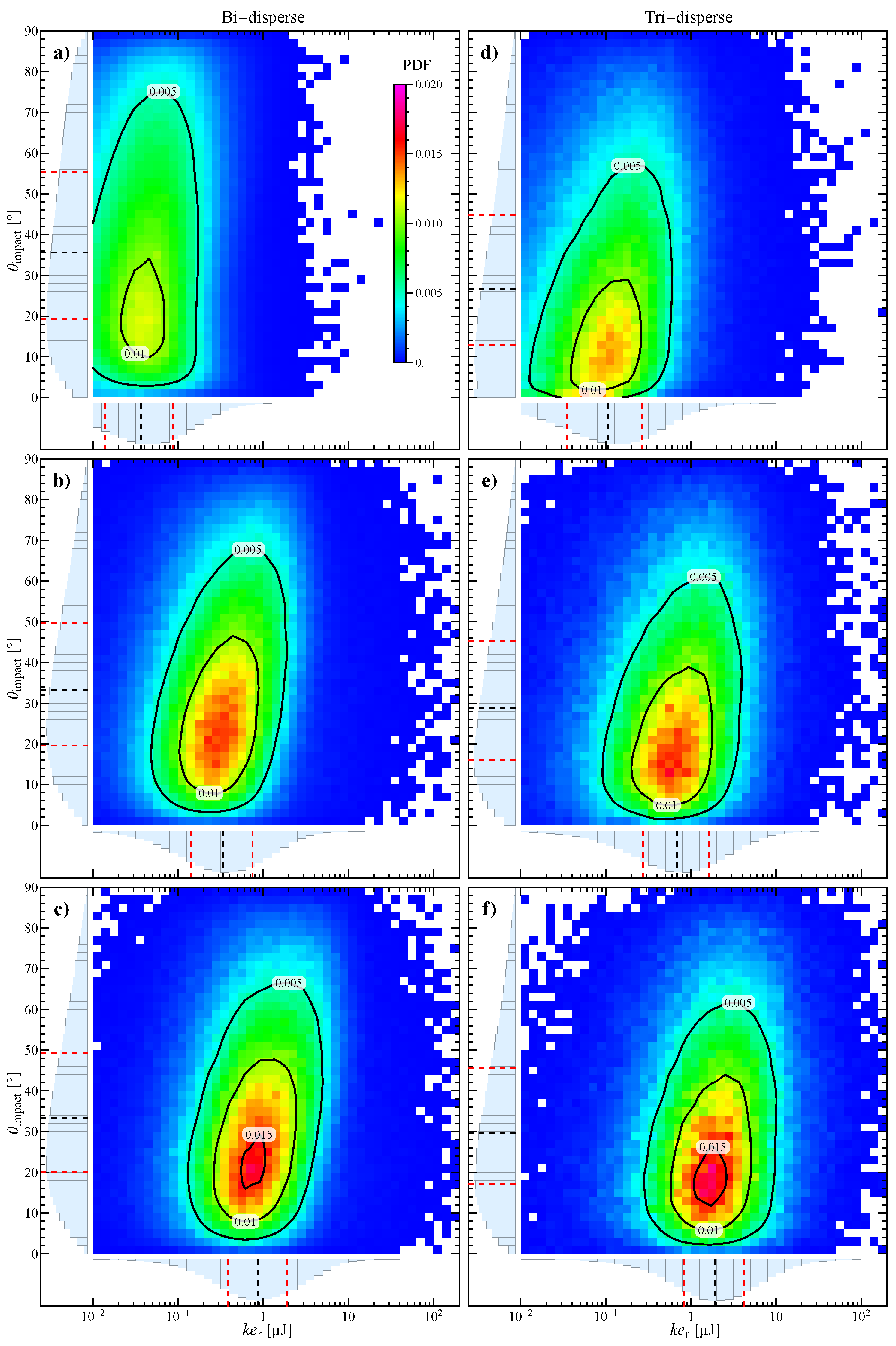
3.4. Effect of Grinding Bead Size

The balance between the size of precursor and grinding beads is a critical aspect of bead milling processes. Indeed, a relatively large inter-bead space in a close packing configuration can dramatically reduce the milling efficiency [10].

In order to reproduce different bed configurations, further simulations were carried out by varying the size and number of grinding beads. In particular, three other systems with fixed total solid volume fraction were considered:

• Bi-disperse, 4 Ag beads of 3 mm and 135 ZrO₂ beads of 2 mm diameter;
• Tri-disperse, 4 Ag beads of 3 mm and 55 ZrO₂ beads of 2 mm and 10 ZrO₂ beads of 4 mm diameter;
• Autogenous, 44 Ag beads of 3 mm diameter.

The comparison among these new systems and the reference in terms of impact kinetic energy, impact angle, and collision frequency is shown in Figure 6, where, for the sake of simplicity, only the median values are reported.

Furthermore, the joint probability density functions of the bi- and tri-disperse systems are shown in Figure 7, while the PDFs of the autogenous system are not reported since they are very similar to the standard case for the overall collisions (left-hand column of Figure 5).

The impact angle was found to be almost independent of the filling configuration, with the greatest variation at low Ω (see, e.g., Figure 7a,d corresponding to Figure 6b at 300 rpm). The detected median value of 30° in the experimental operative regime is then characteristic of the geometry under investigation.

The smaller and more numerous grinding beads of the bi-disperse system induce a reduction in the impact kinetic energy and an increase in the impact frequency (Figure 6). The joint distribution is slightly more spread towards higher ${\theta }_{\mathrm{impact}}$ values (Figure 7).

The tri-disperse system, with fewer small and some large particles, partially recovers in terms of $k{e}_{\mathrm{r}}$, but ${\nu }_{\mathrm{c}}$ is reduced almost to the standard configuration value. The shape of the PDF, which is more similar to the standard case than the bi-disperse one, is in agreement with this observation.

Assuming that a certain level of impact energy must be reached in order to induce abrasion and produce NPs, neither the bi- nor the tri-disperse systems seems to be optimal. Indeed, the same energy level of the standard system can be achieved by increasing the stirring speed, but this determines a reduction in the impact frequency to approximately the same value of the mono-disperse system, thus nullifying the benefits.

A different discussion applies to the autogenous system. Since all the beads are precursors and Ag has a higher density than ZrO₂, if compared to the reference case, the autogenous system has a slightly higher impact energy (Figure 6d) but a much higher useful collision frequency (Figure 6f). Therefore, the autogenous configuration, which presents limitations in the IWM case, turns out to be the optimal choice.

4. Conclusions

In this contribution, a DEM numerical investigation on a novel wet-operating ball mill apparatus for the production of metal NPs has been performed. The innovative configuration of the system allows the synthesis of ferromagnetic NPs despite the magnetically induced agitation. Different stirring velocities and grinding bead sizes at fixed volume fraction have been considered. In particular, their effect on collision energy, angle, and frequency have been analyzed in-depth.

In all the investigated conditions, the system exhibits stable dynamics, characterized by a nearly constant total kinetic energy and collision frequency, with values depending on the stirring velocity. The median of the impact kinetic energy distribution was found to depend on the stirring speed by a power-law with an exponent around 2.5 and is higher for larger beads. On the other hand, the impact angle has an almost constant value of 30°, regardless of the stirring speed and filling configuration. This indicates that, although to a lesser extent than in the inner-bar wet miller (IWM) case, the collision velocity has a predominant tangential component, which has been shown to be more effective in the abrasion of metal particles.

The need to investigate various parameters such as device configurations, materials, and operating conditions makes optimization of this complex system an experimentally difficult, time-consuming, and costly task. In this context, although the adopted approach is limited to the bead scale and thus does not provide direct information on the produced nanoparticles, the obtained results can be a useful resource to guide the design towards the development of more efficient and sustainable NP production processes.

References

1. Khan, I.; Saeed, K.; Khan, I. Nanoparticles: Properties, applications and toxicities. Arab. J. Chem. 2019, 12, 908–931. [Google Scholar] [CrossRef]
2. Viñes, F.; Gomes, J.R.B.; Illas, F. Understanding the reactivity of metallic nanoparticles: Beyond the extended surface model for catalysis. Chem. Soc. Rev. 2014, 43, 4922–4939. [Google Scholar] [CrossRef] [PubMed]
3. Wang, J.; Gu, H. Novel Metal Nanomaterials and Their Catalytic Applications. Molecules 2015, 20, 17070–17092. [Google Scholar] [CrossRef] [PubMed]
4. Stark, W.J.; Stoessel, P.R.; Wohlleben, W.; Hafner, A. Industrial applications of nanoparticles. Chem. Soc. Rev. 2015, 44, 5793–5805. [Google Scholar] [CrossRef]
5. Bao, G.; Mitragotri, S.; Tong, S. Multifunctional Nanoparticles for Drug Delivery and Molecular Imaging. Annu. Rev. Biomed. Eng. 2013, 15, 253–282. [Google Scholar] [CrossRef]
6. Sun, T.; Zhang, Y.S.; Pang, B.; Hyun, D.C.; Yang, M.; Xia, Y. Engineered Nanoparticles for Drug Delivery in Cancer Therapy. Angew. Chem. Int. Ed. 2014, 53, 12320–12364. [Google Scholar] [CrossRef]
7. Nowack, B.; Bucheli, T.D. Occurrence, behavior and effects of nanoparticles in the environment. Environ. Pollut. 2007, 150, 5–22. [Google Scholar] [CrossRef]
8. Yu, L.; Ruan, S.; Xu, X.; Zou, R.; Hu, J. One-dimensional nanomaterial-assembled macroscopic membranes for water treatment. Nano Today 2017, 17, 79–95. [Google Scholar] [CrossRef]
9. Guerra, J.; Herrero, M.A. Hybrid materials based on Pd nanoparticles on carbon nanostructures for environmentally benign C–C coupling chemistry. Nanoscale 2010, 2, 1390. [Google Scholar] [CrossRef]
10. Reverberi, A.P.; Vocciante, M.; Salerno, M.; Ferretti, M.; Fabiano, B. Green Synthesis of Silver Nanoparticles by Low-Energy Wet Bead Milling of Metal Spheres. Materials 2020, 13, 63. [Google Scholar] [CrossRef]
11. Sajid, M.; Ilyas, M.; Basheer, C.; Tariq, M.; Daud, M.; Baig, N.; Shehzad, F. Impact of nanoparticles on human and environment: Review of toxicity factors, exposures, control strategies, and future prospects. Environ. Sci. Pollut. R. 2014, 22, 4122–4143. [Google Scholar] [CrossRef] [PubMed]
12. Alnarabiji, M.S.; Yahya, N.; Hamed, Y.; Ardakani, S.E.M.; Azizi, K.; Klemeš, J.J.; Abdullah, B.; Tasfy, S.F.H.; Hamid, S.B.A.; Nashed, O. Scalable bio-friendly method for production of homogeneous metal oxide nanoparticles using green bovine skin gelatin. J. Clean. Prod. 2017, 162, 186–194. [Google Scholar] [CrossRef]
13. Meramo, S.I.; Bonfante-Alvarez, H.; De Avila-Montiel, G.; Herrera-Barros, A.; Gonzalez-Delgado, A.D. Environmental assessment of a large-scale production of TiO2 nanoparticles via green chemistry. Chem. Eng. Trans. 2018, 70, 1063–1068. [Google Scholar] [CrossRef]
14. Nagar, N.; Devra, V. Green synthesis and characterization of copper nanoparticles using Azadirachta indica leaves. Mater. Chem. Phys. 2018, 213, 44–51. [Google Scholar] [CrossRef]
15. Korir, D.K.; Gwalani, B.; Joseph, A.; Kamras, B.; Arvapally, R.K.; Omary, M.A.; Marpu, S.B. Facile Photochemical Syntheses of Conjoined Nanotwin Gold-Silver Particles within a Biologically-Benign Chitosan Polymer. Nanomaterials 2019, 9, 596. [Google Scholar] [CrossRef] [PubMed]
16. Reverberi, A.; Vocciante, M.; Salerno, M.; Soda, O.; Fabiano, B. A sustainable, top-down mechanosynthesis of carbohydrate-functionalized silver nanoparticles. React. Chem. Eng. 2022, 7, 888–897. [Google Scholar] [CrossRef]
17. Ogi, T.; Zulhijah, R.; Iwaki, T.; Okuyama, K. Recent Progress in Nanoparticle Dispersion Using Bead Mill. KONA Powder Part. J. 2017, 34, 3–23. [Google Scholar] [CrossRef]
18. Beinert, S.; Fragnière, G.; Schilde, C.; Kwade, A. Analysis and modelling of bead contacts in wet-operating stirred media and planetary ball mills with CFD–DEM simulations. Chem. Eng. Sci. 2015, 134, 648–662. [Google Scholar] [CrossRef]
19. Beinert, S.; Fragnière, G.; Schilde, C.; Kwade, A. Multiscale simulation of fine grinding and dispersing processes: Stressing probability, stressing energy and resultant breakage rate. Adv. Powder Technol. 2018, 29, 573–583. [Google Scholar] [CrossRef]
20. Fu, X.; Cai, J.; Zhang, X.; Li, W.D.; Ge, H.; Hu, Y. Top-down fabrication of shape-controlled, monodisperse nanoparticles for biomedical applications. Adv. Drug Deliver. Rev. 2018, 132, 169–187. [Google Scholar] [CrossRef] [PubMed]
21. Ali, M.E.; Ullah, M.; Maamor, A.; Hamid, S.B.A. Surfactant Assisted Ball Milling: A Simple Top down Approach for the Synthesis of Controlled Structure Nanoparticle. Adv. Mat. Res. 2013, 832, 356–361. [Google Scholar] [CrossRef]
22. Ullah, M.; Ali, M.; Hamid, S.B.A. Surfactant-assisted ball milling: A novel route to novel materials with controlled nanostructure—A review. Rev. Adv. Mater. Sci. 2014, 37, 1–14. [Google Scholar]
23. Trofa, M.; D’Avino, G.; Fabiano, B.; Vocciante, M. Nanoparticles Synthesis in Wet-Operating Stirred Media: Investigation on the Grinding Efficiency. Materials 2020, 13, 4281. [Google Scholar] [CrossRef] [PubMed]
24. Trofa, M.; Reverberi, A.P.; Vocciante, M. Discrete Element Method Simulations of an Innovative Magnetic Stirred Device for the Top-down Production of Ferromagnetic Nanoparticles. Chem. Eng. Trans. 2023, 100, 121–126. [Google Scholar] [CrossRef]
25. Marshall, J.S.; Li, S. Adhesive Particle Flows: A Discrete-Element Approach; Cambridge University Press: New York, NY, USA, 2014. [Google Scholar] [CrossRef]
26. Blau, P.J. The significance and use of the friction coefficient. Tribol. Int. 2001, 34, 585–591. [Google Scholar] [CrossRef]
27. Fragnière, G.; Beinert, S.; Overbeck, A.; Kampen, I.; Schilde, C.; Kwade, A. Predicting effects of operating condition variations on breakage rates in stirred media mills. Chem. Eng. Res. Des. 2018, 138, 433–443. [Google Scholar] [CrossRef]
28. Smith, D.R.; Fickett, F.R. Low-Temperature Properties of Silver. J. Res. Natl. Inst. Stand. Technol. 1995, 100, 119. [Google Scholar] [CrossRef]
29. Gondret, P.; Lance, M.; Petit, L. Bouncing motion of spherical particles in fluids. Phys. Fluids 2002, 14, 643–652. [Google Scholar] [CrossRef]
30. Stronge, W.J. Impact Mechanics; Cambridge University Press: Cambridge, UK, 2018. [Google Scholar] [CrossRef]
31. Vocciante, M.; Trofa, M.; D’Avino, G.; Reverberi, A.P. Nanoparticles Synthesis in Wet-operating Stirred Media: Preliminary Investigation with Dem Simulations. Chem. Eng. Trans. 2019, 73, 31–36. [Google Scholar] [CrossRef]
32. Kloss, C.; Goniva, C.; Hager, A.; Amberger, S.; Pirker, S. Models, algorithms and validation for opensource DEM and CFD–DEM. Prog. Comput. Fluid Dyn. 2012, 12, 140–152. [Google Scholar] [CrossRef]
33. Bitter, J.G.A. A study of erosion phenomena. Wear 1963, 6, 169–190. [Google Scholar] [CrossRef]
34. Sheldon, G.L. Similarities and Differences in the Erosion Behavior of Materials. J. Basic Eng. ASME 1970, 92, 619–626. [Google Scholar] [CrossRef]
35. Hutchings, I.; Shipway, P. Tribology: Friction and Wear of Engineering Materials; Butterworth-Heinemann, an imprint of Elsevier: Oxford, UK, 2017; p. 412. [Google Scholar]
Figure 1. (a) Schematic representation of the outer-bar wet miller (OWM). (b) Simulation domain showing the L-bent rotating glass shaft and the ZrO2 (yellow) and Ag (blue) beads. Adapted from [24].
Applsci 14 01550 g001
Figure 2. Total (a) translational and (b) rotational kinetic energy at different stirring velocities. Each curve is the average of six simulations with different random seeds.
Applsci 14 01550 g002
Figure 3. (a,d) Impact kinetic energy, (b,e) impact angle, and (c,f) collision frequency as a function of the stirring velocity. The left column refers to collisions between all particles in the system, while the right column refers to those involving at least one Ag particle. In the first and second row, the median, first, and third quartiles of the distribution are shown.
Applsci 14 01550 g003
Figure 4. (a) Impact kinetic energy, (b) impact angle, and (c) ratios of kinetic energy and frequency as a function of the stirring velocity for the collisions between the beads and the container wall. In the first and second panel, the median, first, and third quartiles of the distribution are shown.
Applsci 14 01550 g004
Figure 5. Density histogram and contour plot of the joint probability density function for impact angle and impact kinetic energy at (a,d) 300 rpm, (b,e) 600 rpm, and (c,f) 900 rpm. The left column refers to collisions between all particles in the system, while the right column refers to those involving at least one Ag particle. On the edges of each map, the marginal probability density functions and the corresponding quartiles are also shown (the median in black and the first and third quartiles in red).
Applsci 14 01550 g005
Figure 6. Comparison of the investigated grinding systems in terms of (a,d) impact kinetic energy, (b,e) impact angle, and (c,f) collision frequency as a function of the stirring velocity. The left column refers to collisions between all particles in the system, while the right column refers to those involving at least one Ag particle.
Applsci 14 01550 g006
Figure 7. Density histogram and contour plot of the joint probability density function for impact angle and impact kinetic energy at (a,d) 300 rpm, (b,e) 600 rpm, and (c,f) 900 rpm for the bi-disperse (left column) and tri-disperse (right column) system. On the edges of each map, the marginal probability density functions and the corresponding quartiles are also shown (the median in black and the first and third quartiles in red).
Applsci 14 01550 g007