TSE-UNet: Temporal and Spatial Feature-Enhanced Point Cloud Super-Resolution Model for Mechanical LiDAR

Abstract

The mechanical LiDAR sensor is crucial in autonomous vehicles. After projecting a 3D point cloud onto a 2D plane and employing a deep learning model for computation, accurate environmental perception information can be supplied to autonomous vehicles. Nevertheless, the vertical angular resolution of inexpensive multi-beam LiDAR is limited, constraining the perceptual and mobility range of mobile entities. To address this problem, we propose a point cloud super-resolution model in this paper. This model enhances the density of sparse point clouds acquired by LiDAR, consequently offering more precise environmental information for autonomous vehicles. Firstly, we collect two datasets for point cloud super-resolution, encompassing CARLA32-128in simulated environments and Ruby32-128 in real-world scenarios. Secondly, we propose a novel temporal and spatial feature-enhanced point cloud super-resolution model. This model leverages temporal feature attention aggregation modules and spatial feature enhancement modules to fully exploit point cloud features from adjacent timestamps, enhancing super-resolution accuracy. Ultimately, we validate the effectiveness of the proposed method through comparison experiments, ablation studies, and qualitative visualization experiments conducted on the CARLA32-128 and Ruby32-128 datasets. Notably, our method achieves a PSNR of 27.52 on CARLA32-128 and a PSNR of 24.82 on Ruby32-128, both of which are better than previous methods.

1. Introduction

LiDAR (light detection and ranging) plays a pivotal role in intelligent robots, autonomous vehicles, and unmanned aerial vehicles (UAVs), as it provides precise distance measurements of the surrounding environments, making it one of the most essential sensors. It is fundamental to the operation of these advanced technologies, enabling them to navigate safely, avoid obstacles, and make informed decisions about their movements. Without LiDAR, these machines would lack the necessary data to function properly, severely limiting their capabilities and reliability. Therefore, LiDAR’s role in fields such as robotics, autonomous driving, and unmanned aerial vehicles is crucial, making it a vital component for the development of advanced and safe technologies [1,2].

Currently, LiDAR sensors available off-the-shelf can be classified into two main categories: mechanical LiDAR and solid-state LiDAR [3]. Over the past few decades, mechanical LiDAR has been extensively utilized in various applications and environments because of its design, which incorporates a 360-degree horizontal field of view (FOV). This broad FOV allows mechanical LiDAR to capture comprehensive information about the surrounding environment within a single scan. The vertical FOV is determined by the number of included laser beams and the angle between adjacent laser beams, which is also referred to as angular resolution. Mechanical LiDAR offers numerous advantages, such as its ability to obtain all surrounding information within a single scan. This design enables it to acquire data quickly and efficiently, making it suitable for a range of applications, including autonomous vehicles, robotics, and surveying. However, the predefined angular resolutions in both the horizontal and vertical directions can limit the resolution of perception, particularly in the horizontal angular resolution. As the distance increases, the spacing between each laser beam also increases, resulting in sparse features in the final 3D point cloud. To address these limitations, solid-state LiDAR was developed using non-repetitive scanning technology. This technology concentrates all the laser beams within a limited field of view, enabling dense scanning over a specific time interval. By focusing the laser beams in a limited FOV, solid-state LiDAR can achieve dense scanning without sacrificing the overall field of view range. This approach offers improved resolution compared to mechanical LiDAR, as it utilizes non-repetitive scanning patterns. Despite its advantages, solid-state LiDAR also has certain trade-offs. To achieve non-repetitive scanning, complex mechanical structures are required, which can reduce the final ranging accuracy of the sensor. Additionally, the limited field of view can be a constraint in some applications where a wide FOV is essential. To achieve a full 360-degree horizontal sensing capability, multiple LiDAR sensors, sophisticated installation structures, and synchronization algorithms are often required [4].

To overcome the shortcomings of mechanical liDAR in practical applications, we delve into recent advances in point cloud [5,6,7], image-based super-resolution technology [8,9], and deep-learning-based modeling [10,11], which can provide new ideas and methods to solve the limitations of mechanical LiDAR. First of all, as the main data form of LiDAR environment perception, the point cloud has accurate 3D information. However, because of the scanning method of mechanical LiDAR, the obtained point clouds are usually very sparse, which poses challenges for subsequent algorithms. Therefore, we consider using point cloud super-resolution technology. By using multi-frame continuous LiDAR scanning data combined with image processing and machine learning methods, the point cloud is interpolated and upsampled. This can improve the density of the point cloud to a certain extent and provide more accurate environmental information for the subsequent perception algorithm. The traditional point cloud super-resolution technology has the problems of heavy computation and poor real-time performance. By building a deep neural network model to learn and predict the point cloud data, a denser point cloud can be restored to a certain extent. In order to better adapt to the scanning line characteristics of mechanical LiDAR, we propose a new mechanical LiDAR point cloud super-resolution model, TSE-UNet. The model combines the U-Net structure and the characteristics of temporal and spatial feature-enhanced modules to optimize the scanning line characteristics of mechanical LiDAR. TSE-UNet can capture the time dynamics of the point cloud effectively and recover the high-density point cloud with spatial feature-enhanced skip connection and upsampling operations. In addition, TSE-UNet uses a lightweight network structure and efficient convolution algorithm to achieve efficient point cloud super-resolution in real time with lightweight edge computing devices. With our model, sparse point clouds captured by low-cost liDAR (i.e., Robosense-32) can be enhanced in real time with lightweight edge computing devices. In addition, upsampled point clouds can achieve similar results compared to point clouds of high-cost LiDAR (i.e., Robosense-128). Our TSE-UNet model can easily scale sparse point clouds from low-cost LiDAR sensors to dense point clouds with dense laser beams, thereby improving the performance of subsequent point cloud-based perception modules.

The contributions of this paper are as follows:

• To address the shortage of available open-source datasets in the field, we construct and release a simulation dataset, CARLA32-128, for a laser beam LiDAR point cloud super-resolution task. Additionally, a real-world dataset, Ruby32-128, is provided for the 32-to-128 laser beam LiDAR point cloud super-resolution task.
• Based on the semantic segmentation model UNet, we propose a temporal and spatial feature-enhanced point cloud super-resolution model called TSE-UNet. It utilizes a temporal feature attention aggregation module and a spatial feature enhancement module to fully leverage point cloud features from neighboring timestamps, improving super-resolution accuracy.
• We validate the effectiveness of the proposed method through extensive comparative experiments, ablation experiments, and visual qualitative experiments.

The rest of this paper is organized as follows. Section 2 reviews the related works on image super-resolution and point cloud super-resolution. Section 3 presents the detailed design of the TSE-UNet model, and Section 4 evaluates the model on both synthetic data captured in the CARLA simulator and real-world data collected from a local vehicle platform. Section 5 summarizes this work.

2. Related Works

2.1. Image Super-Resolution

Image super-resolution is a traditional task in computer vision involving the use of algorithms to enhance low-resolution images to high-resolution ones. This technique finds applications in various fields, such as surveillance, medical imaging, and media. Its advantage lies in the ability to effectively improve the outcomes of subsequent tasks, such as face recognition and semantic segmentation, without increasing sensor hardware costs. In past research, various techniques have been developed, encompassing regularization techniques [12], neighborhood embedding-based algorithms [13], and the utilization of similar patches that exhibit redundancy in low-resolution images when compared to their higher-resolution counterparts. Nonetheless, these methods are not optimal and encounter challenges when applied to tasks involving higher-scale images.

Simultaneously, with the continuous development of deep learning technology, [14] were the first to apply convolutional neural networks (CNNs) to this task. They employed a lightweight deep CNN for end-to-end learning on the data, achieving state-of-the-art results in both quality and speed. The observation that deeper networks for super-resolution (SR) are challenging to train, coupled with the underutilization of abundant information in feature maps across various layers, led to the proposition of residual channel attention networks (RCANs) [15]. The residual-in-residual (RIR) structure facilitates the bypassing of copious low-frequency information through multiple skip connections, enabling the primary network to concentrate on learning high-frequency information. Moreover, attention mechanisms [16,17] targeting spatial or channel dimensions have been incorporated to enhance the model’s capacity for improved representation. Recently, the Transformer [18] has shown remarkable performance in high-level vision tasks. It reveals that both spatial and channel information are important for performance. Pre-trained Transformer models [19,20] have also been proposed, and their effectiveness has been validated in the context of SR tasks. ESSAformer [21] was proposed as a Transformer network embedded with ESSA attention for single hyperspectral image super-resolution, featuring an iterative refining structure. Remarkably, ESSA achieved significant improvements in both visual quality and quantitative results in experiments, all without the necessity of pretraining on large datasets.

2.2. Point Cloud Super-Resolution

Point cloud super-resolution is similar to image super-resolution, employing super-resolution techniques to increase the density of points in a low-density point cloud. T-UNet [22] was designed as a point cloud super-resolution network utilizing an encoder–decoder framework that integrates temporal features. However, it simply incorporates temporal information directly without fully exploiting its potential. Therefore, there is room for improvement by introducing advanced feature processing methods [23,24] into the encoder to enhance feature extraction capabilities. Consequently, there is still potential for improvement in fully utilizing temporal and spatial features. Pu-net [25] explores multi-level features for each point by implicitly expanding the point set through a multi-branch convolution unit in feature space. The augmented feature is subsequently partitioned into numerous features, which are later reconstructed to form a super-resolution point set. PUGeo-Net [26] is a deep learning method based on geometric transformations that learns local parameters and normals for each point. Through sampling in the 2D parameter domain and utilizing the learned 3D transformations, the point cloud is upsampled, achieving precise and efficient results at super-resolution rates ranging from 4 to 16 times. Sspu-net [27] for self-supervised point cloud upsampling leverages the coherence between the initial sparse point cloud and the resultant dense point cloud in terms of shapes and rendered images. Meta-PU [28] is the first implementation supporting arbitrary-scale point cloud upsampling using a single model. This model integrates residual graph convolution blocks, a meta-subnetwork, and the farthest sampling block. Notably, Meta-PU surpasses the performance of existing methods, which are typically trained for specific scale factors. While these approaches do offer qualitative results for LiDAR point clouds, their emphasis is on augmenting the overall 3D point density of point clouds pertaining to individual objects rather than addressing larger scenes. LiDAR super-resolution aims to replicate a realistic point cloud resembling that of a high-beams LiDAR, given the point cloud from a low-beams LiDAR. As a result, its objective differs from the aforementioned approaches.

Given the challenges and substantial computational requirements associated with upsampling LiDAR point clouds in 3D space, the majority of studies opt to represent the point cloud as a range image. Consequently, the LiDAR super-resolutions task is conducted within the confines of 2D image space. Ref. [29] employed a CNN with a U-Net architecture. Furthermore, it incorporates a Monte-Carlo dropout post-processing step to mitigate the presence of noisy points in the predictions. Local implicit image function (LIIF) [30] treats an image as a continuous function, positing that the RGB values of discrete pixel points are calculated by a function taking pixel position and depth as inputs. This function is approximated using a multi-layer perceptron. The model proposed in ref. [31] takes a range image from a point cloud as input and undergoes operations, including encoding, to predict parameters. The model also incorporates a self-attention mechanism. In comparison to directly using LIIF for image prediction, it exhibits fewer noise artifacts. HALS [32] also takes a range image as input after several rounds of dilated residual blocks (DRBs) for feature extraction and diverges into two paths. One path directly undergoes upsampling to generate the final result, while the other path continues with DRBs to generate deeper features before further upsampling. These two paths represent shadow and deep information, and they are finally combined through point-wise addition.

3. Method

The cost of multi-beam LiDAR has always been a significant obstacle to the widespread adoption of autonomous driving and mobile intelligent robots. The point clouds captured by low-cost LiDAR are typically sparse and have low resolution, which limits the performance of deep learning models and makes data annotation more challenging. Furthermore, we consider that the collection of point clouds comes from moving autonomous vehicles or mobile intelligent robots, which means that the point cloud data with spatial information also possesses temporal information. Our objective is to generate stable and accurate dense point clouds of road scenes from consecutive sparse point clouds with temporal features. To achieve this, we propose a TSE-UNet model designed for upsampling the point cloud from low-cost LiDAR, specifically for the task of point cloud super-resolution.

The entire pipeline of the proposed method is illustrated in Figure 1. Firstly, datasets for training and evaluating the model performance are collected on both the CARLA simulator and our real-world platform, including CARLA32-128 (with 128 laser beams, RS-128) and Ruby32-128 (with 128 laser beams, RS-128). Subsequently, we transform the point cloud super-resolution task from a 3D spatial interpolation problem to a 2D image super-resolution problem, reducing the computational complexity of the deep learning model and enabling real-time application. Specifically, based on coordinate mapping, we project 3D sparse point clouds onto 2D projection sequential images and then encode the 2D images into feature maps using transposed convolution layers. Following this, we process the feature maps using the proposed TSE-UNet model. This model, built upon the encoder–decoder structure of UNet, takes multiple consecutive frames as input, representing multiple consecutive feature maps. We combine feature maps from two adjacent frames, enhance important features temporally using channel attention modules, and reinforce spatial correlations between adjacent frames using spatial attention modules, providing more accurate object localization and semantic information. The encoder further increases spatial receptive fields and downsamples features through dilated convolution layers, progressively extracting high-level semantic features. The decoder starts from the highest-level semantic feature map of the encoder to restore low-level semantics, ultimately outputting the super-resolution prediction for the current frame. Finally, the obtained prediction results are mapped back to 3D space through reverse projection. Subsequent sections provide detailed explanations of each part of the pipeline.

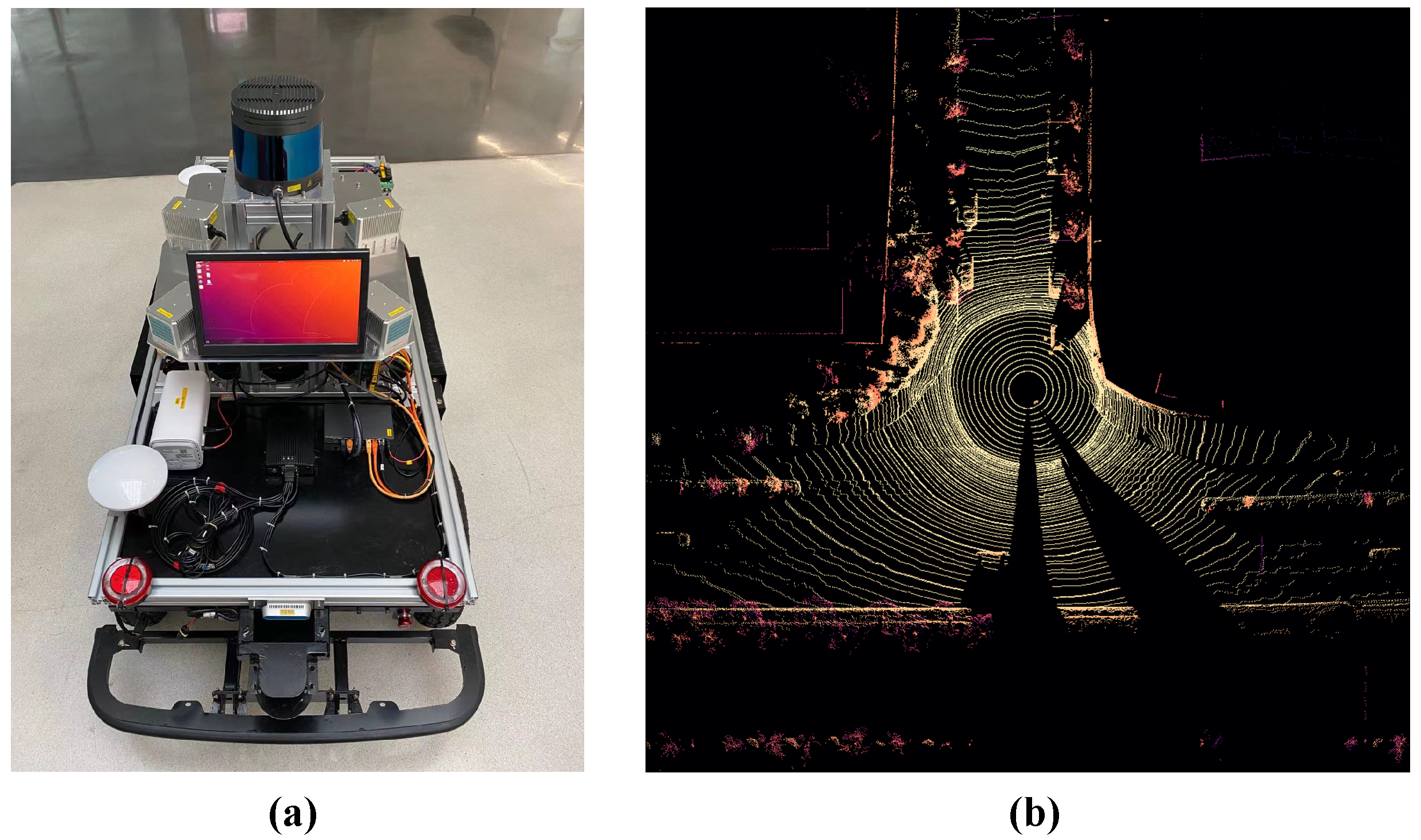
3.1. Data Collection

We introduce the two datasets we constructed for the point cloud super-resolution task. One dataset was collected from the CARLA [33] driving simulator, named CARLA32-128, and the other was collected from real scenes, called Ruby32-128. The detailed information of the datasets is shown in

Table 1. Detailed information for the CARLA32-128 and Ruby32-128 datasets. Note that CARLA32-128 comprises CARLA32 and CARLA128; Ruby32-128 is composed of Ruby32 and Ruby128.

Names	Number of Frames	Laser Beams	FOV (Vertical)
CARLA32	7025	32	(−25°, 15°)
CARLA128	7025	128	(−25°, 15°)
Ruby-32	2402	32	(−25°, 15°)
Ruby-128	2402	128	(−25°, 15°)

.

3.1.1. Simulation Scenario

CARLA (Car Learning to Act) is an open-source simulator used for the development and testing of autonomous driving systems. It provides a highly configurable virtual urban environment with real road networks, diverse traffic participants, various weather conditions, and rich urban scenes and is shown in Figure 2a. The CARLA simulator simulates the working principle of LiDAR accurately, including the process of laser beam emission and reception, as well as the vertically defined sensor field of view (FOV) and 360-degree horizontal FOV. We used the LiDAR in the simulator to collect 7025 frames of 128-line point cloud data. The bird’s eye view of the point cloud is shown in Figure 2b. Then, we downsampled the 128-line point cloud data 4 times to obtain 32-line point cloud data, thus creating 32-line and 128-line point cloud data pairs. Each pair of data is a data sample of the point cloud super-resolution task. The collected dataset is named CARLA32-128. Detailed information about the number of frames, laser beams, and vertical perspective is shown in Table 1.

3.1.2. Real Scenario

In addition to collecting data in simulation scenarios, we also built a LiDAR point cloud acquisition platform based on real scenes with a RoboSense Ruby (with 128 laser beams, RS-128). According to different azimuth and vertical angle settings, the non-uniform laser beam LiDAR used in our platform makes the projection point cloud acquisition very flexible. Figure 3a shows the experimental vehicle platform with RS-32/RS-128 and other equipment. We used this platform to collect synchronized 128-line data and downsampled the 128-line point cloud data 4 times to obtain 32-line point cloud data, constructing a dataset called Ruby32-128 for the 2402 pairs of 32-line to 128-line point cloud super-resolution task. Detailed information about the number of frames, laser beams, and vertical perspective is shown in Table 1, and the bird-view images of the collected point cloud are shown in Figure 3b.

3.2. Point Cloud Projection and Back-Projection

The density of point clouds varies with different laser beams and rotating speeds of LiDAR, resulting in different vertical angular resolution and horizontal angular resolution. Based on the 3D coordinates ($x,y,z$) of point clouds and the vertical angle ($\omega$), azimuth angle ($\alpha$), and offset ($\delta$), we project the point clouds in 3D space onto a two-dimensional plane according to Equation (1), making it easier to process these data using deep learning methods based on two-dimensional images. Subsequently, we use Equation (2) to back-project the processed prediction results from the model into 3D space.

$$\begin{array}{c}r=\sqrt[]{x^2+y^2+z^2},\hfill \\ \alpha +\delta =arctan(y/x),\hfill \\ \omega =arcsin(z/r).\hfill \end{array}$$

(1)

$$\begin{array}{c}x=rcos\left(\omega \right)sin(\alpha +\delta ),\hfill \\ y=rcos\left(\omega \right)cos(\alpha +\delta ),\hfill \\ z=rsin\left(\omega \right).\hfill \end{array}$$

(2)

Figure 4 illustrates the results of projecting 3D point cloud data from CARLA32-128 and Ruby32-128 onto 2D images. It can be observed that the widths of the corresponding 2D images are the same for CARLA-32 and CARLA-128 because of their identical horizontal FOV and angular resolution during data acquisition. However, the difference lies in the heights of the 2D images, with the image for CARLA-128 being four times taller than that for CARLA-32, as shown in the first and second rows of Figure 4. Similarly, Ruby-32 and Ruby-128, shown in the third and fourth rows of Figure 4, share the same characteristics. Therefore, our TSE-UNet model aims to recover dense point clouds from sparse ones.

3.3. TSE-UNet Model

To reconstruct a dense point cloud from a sparse point cloud, the model needs to have the ability to extract features and high-level semantic understanding from the sparse point cloud, as well as the ability to reconstruct high-level semantics into fine-grained low-level information, to achieve point cloud super-resolution. This process coincides with the design idea of the semantic segmentation model UNet. In addition, because the point cloud is dynamically collected by an autonomous vehicle, the semantic information of a certain frame of point cloud has a strong correlation with the semantic information of the previous frames of point cloud; at the same time, a certain point on the current frame of point cloud has a strong spatial correlation with the surrounding point cloud. Therefore, we propose a method combining the TSE module with UNet, namely TSE-UNet, to achieve the task of point cloud super-resolution. Figure 5 shows the architecture of the TSE-UNet.

TSE-UNet incorporates the encoder–decoder structure and skip connections of UNet while introducing temporal feature attention aggregation modules and spatial feature enhancement modules.

The encoder is responsible for extracting high-level semantic features from point cloud data. The encoder consists of a pre-processing layer and four stages.

The input to the pre-processing layer includes the current frame and the projected images of the previous 15 frames, denoted as $T=\{T_i\mid i\in \{0,1,\dots ,15\}\}$, where the dimension of $T_i$ is $H\times W\times C$. The pre-processing layer applies the following formula to each input image:

$$\begin{array}{c}\hfill T_i^{\prime }=\mathit{TConv}\left(\mathit{TConv}\left(T_i\right)\right),\end{array}$$

(3)

where $\mathit{TConv}$ represents the transposed convolution operation with a stride of 2 in the height dimension. The dimension of $T_i^{\prime }$ is $D\times W\times C$, where $D=4\times H$. The purpose of the pre-processing is to increase the height of the sparse point cloud image to four times its original size, aligning it with the height of the dense point cloud for pixel-level predictions.

The structure is consistent across the four stages, comprising adjacent temporal feature aggregation, temporal and spatial feature-enhanced modules, and a down-sampling large-scale dilated convolution. Taking the operations on $T_0$ and $T_1$ in stage 1 as an example, the computation for the adjacent temporal feature aggregation operation is given by the following formula:

$$\begin{array}{c}\hfill F_{01}=\mathit{Concat}(T_0^{\prime },T_1^{\prime }),\end{array}$$

(4)

where $\mathit{Concat}$ denotes the concatenation operation along the depth dimension, resulting in $F_{01}$ with dimensions $D\times W\times 2C$.

Subsequently, through the temporal and spatial feature-enhanced (TSE) module,

$$\begin{array}{c}{X}_{01}=\mathit{Conv}\left(F_{01}\right),\hfill \\ \overline{X_{01}}=\sigma \left(\mathit{favg}\left(X_{01}\right)\right)\odot X_{01},\hfill \\ \widehat{X_{01}}=\sigma \left(\mathit{PConv}\left(X_{01}\right)\right)\odot \overline{X_{01}},\hfill \end{array}$$

(5)

where $\mathit{Conv}$ represents a 2D convolution with a kernel size of 3 and a stride of 1, utilized to further integrate features between adjacent frames. $\sigma$ denotes the sigmoid function. $\mathit{favg}$ represents channel-wise average pooling, which calculates the importance of temporal features in the channel dimension and injects it into the original features through element-wise multiplication (⊙), thereby achieving temporal feature enhancement. $\mathit{Pconv}$ is a point-wise convolution with a kernel size of 1, a stride of 1, and an output dimension of 1, used to assess the importance of spatial dimensions and inject it into the original features through element-wise multiplication, completing spatial feature enhancement. The TSE module maintains the feature dimensions at $D\times W\times 2C$. Then, the computation continues with the following formula:

$$\begin{array}{c}\hfill O_{01}=\mathit{DConv}\left(\widehat{X_{01}}\right),\end{array}$$

(6)

where $\mathit{DConv}$ denotes a dilated convolution with a kernel size of 3, a stride of 2, and a dilation rate of 2, employed to enlarge the receptive field while accomplishing feature downsampling. The resulting feature $O_{01}$ has dimensions $D/2\times W/2\times 2C$. At this point, the calculation of adjacent frame features in a single stage is complete. The computation in other stages within the encoder and between other adjacent frames follows a similar procedure.

The decoder also consists of four stages, each including a feature upsampling layer, producing features with the same dimensions as the corresponding encoder level. This allows the features to be concatenated and continue participating in the computation. The encoder ultimately outputs a prediction output (denoted as P) with dimensions $D\times W\times C$. This output, along with the dense point cloud projection image corresponding to the input $T_0$ (current frame) through the SSIM (structural similarity index measure) calculation, is denoted as G. The calculation formula for the value of $\mathit{SSIM}$ is as follows:

$$\begin{array}{c}\hfill \mathit{SSIM}(G,P)=\frac{(2{\mu }_G{\mu }_P+C_1)(2{\sigma }_{GP}+C_2)}{({\mu }_G^2+{\mu }_P^2+C_1)({\sigma }_G^2+{\sigma }_P^2+C_2)},\end{array}$$

(7)

where $G{\mu }_G$ and ${\mu }_P$ represent the mean values of the images G and P, respectively; ${\sigma }_G^2$ and ${\sigma }_P^2$ are their variances; and ${\sigma }_{GP}$ is the covariance. $C_1$ and $C_2$ are constants used to prevent division by zero in the denominator. In practical applications, the loss value is computed as $1-\mathit{SSIM}$, where a smaller value indicates greater similarity between images. Subsequently, all model parameters are optimized through backpropagation.

4. Experiments

4.1. Datasets and Evaluation Metrics

We used CARLA32-128 and Ruby32-128, which are described in Section 3.1, to verify the effectiveness of our methods. We randomly split both datasets into training sets and testing sets, with the specific sample numbers shown in

Table 2. The number of frames in the training and testing sets for CARLA32-128 and Ruby32-128.

Names	Number of Training Frames	Number of Testing Frames
CARLA32-128	5162	1863
Ruby32-128	1456	946

.

We chose the PSNR (peak signal-to-noise ratio) and SSIM (structural similarity index measure) loss as the evaluation metrics. The PSNR is extended from MSE (mean square error) and describes the ratio between the maximum possible power of a signal and the power of corrupting noise, which affects the fidelity of its representation. The higher the PSNR, the better the consistency between the generated data and ground truth. It is defined as follows:

$$\begin{array}{c}PSNR=10·{log}_{10}\left(\frac{MA{X}_I^2}{MSE}\right),\hfill \\ MSE=\frac{1}{mn}\sum _{i=0}^{m-1}\sum _{j=0}^{n-1}{[I_1(i,j)-I_2(i,j)]}^2,\hfill \end{array}$$

(8)

where $MA{X}_I$ represents the maximum pixel value of the whole image and $I_1(i,j)$ and $I_2(i,j)$ are two images of the same shape. m and n are the width and height of the projected image. The SSIM loss is the value of the average loss for the testing images. A lower SSIM loss implies a closer resemblance between the model’s predictions and the ground truth.

4.2. Implementation Details

In all experiments, we upsampled the projected point cloud image four times (32 to 128) as the input of the TSE-UNet model. Because of memory constraints, we set the batch size to one during the training phase. To regularize the model and prevent overfitting, we used $L2$ as the regularization term. We used the Adam optimizer with a learning rate of 0.0001 to train the model for 60 epochs and selected the model with the best performance on the test set.

4.3. Comparison Experiments

We chose four methods for comparison. The first one was the classic semantic segmentation method UNet [34]; the second one was the point cloud super-resolution model T-UNet [22] with the ability to process point cloud temporal features; the third one was the LKA-T-UNet [23], which introduces the capability of long-distance spatial feature modeling based on T-UNet; the fourth one was the SMT-T-UNet [24], which introduces multi-scale spatial attention based on T-UNet. The experimental results on the two datasets we proposed are shown in

Table 3. The PSNR and SSIM loss of different models on the CARLA32-128 and Ruby32-128 datasets. Bold indicates the best result.

Datasets	Methods	PSNR	SSIM Loss
	UNet	25.11	30.99 $\times {10}^{-5}$
	T-UNet	26.97	11.89 $\times {10}^{-5}$
CARLA32-128	LKA-T-UNet	27.01	9.61 $\times {10}^{-5}$
	SMT-T-UNet	27.24	12.40 $\times {10}^{-5}$
	TSE-UNet (ours)	27.52	$\mathbf{8.38}\times {\mathbf{10}}^{-\mathbf{5}}$
	UNet	23.96	24.26 $\times {10}^{-5}$
	T-UNet	24.78	14.68 $\times {10}^{-5}$
Ruby32-128	LKA-T-UNet	24.75	14.49 $\times {10}^{-5}$
	SMT-T-UNet	24.80	14.45 $\times {10}^{-5}$
	TSE-UNet (ours)	24.82	$\mathbf{14.32}\times {\mathbf{10}}^{-\mathbf{5}}$

. As can be seen, the method we proposed achieved the best PSNR and the lowest SSIM loss value on both simulated scene and real scene datasets. The results indicate the proposed temporal feature attention aggregation module and spatial feature enhancement module in this paper are designed to fully exploit the temporal and spatial information between consecutive point clouds, leading to improved point cloud super-resolution performance.

4.4. Ablation Study

We conducted ablation experiments on various components of the CARLA32-128 dataset. Since TSE-UNet is based on UNet, we gradually added the key components used in this method to the original UNet network, ultimately forming the TSE-UNet model. The experimental results are shown in

Table 4. Ablation experiments on key components of TSE-UNet using the CARLA32-12 dataset. “T” represents the utilization of temporal information, specifically, the 16 sequential frames used in TSE-UNet; “TE” represents the temporal information enhancement module, and “SE” signifies the spatial information enhancement module. “×” and “✓” indicate non-usage and usage of the respective modules. Higher PSNR values are preferable, while lower SSIM losses indicate improved performance. Optimal values are in bold.

Methods	Components			PSNR	SSIM Loss
	T	TE	SE
UNet	×	×	×	25.11	30.99 $\times {10}^{-5}$
Variant 1	✓	×	×	26.97	11.89 $\times {10}^{-5}$
Variant 2	✓	✓	×	27.38	9.16 $\times {10}^{-5}$
TSE-UNet	✓	✓	✓	27.52	$\mathbf{8.38}\times {\mathbf{10}}^{-\mathbf{5}}$

. The original UNet achieved a PSNR of 25.11 and an SSIM of $30.99\times {10}^{-5}$; when combined with temporal information (Variant 1 model in the table), PSNR improved to 26.97, while SSIM decreased to $11.89\times {10}^{-5}$. Furthermore, after applying the temporal feature attention module (Variant 2 model in the table), PSNR improved to 27.38, while SSIM decreased to $9.16\times {10}^{-5}$; when applying the spatial feature attention module, the model expanded to TSE-UNet, with a PSNR of 27.52 and an SSIM of $8.38\times {10}^{-5}$, which are improved by 2.41 and reduced by $22.61\times {10}^{-5}$, respectively, compared to the original UNet.

4.5. Visualization

We present the point cloud super-resolution visualization results of TSE-UNet. As shown in Figure 6, the first column is the visualization of sparse point clouds as input, the second column is the corresponding dense point clouds ground truth, and the third column is the point cloud super-resolution prediction result of TSE-UNet. As can be seen from the figure, compared with the ground truth of dense point clouds, the upsampled point cloud had some noise points, but it still generated more effective points than the original sparse point cloud. This could provide more abundant environmental information for autonomous vehicles or intelligent robots.

4.6. Speed Performance

Computational latency and real-time performance are among the key factors to consider when deploying point cloud processing algorithms on the computing platform of autonomous vehicles. This subsection tests the processing efficiency of the TSE-UNet model, including latency and frequency. We used a single NVIDIA RTX A5000 (Nvidia Corporation, Santa Clara, CA, USA) as the running platform, performing this experiment on 1000 images on the two datasets proposed in this paper, and the results were averaged. The results are summarized in

Table 5. Average computational latency and frequency of TSE-UNet model on point cloud super-resolution for different datasets.

Datasets	CARLA32-128	Ruby32-128
Latency	21.22 ms	23.85 ms
Frequency	47.12 Hz	41.92 Hz

. It can be seen from the table that the proposed TSE-UNet achieved real-time performance on different datasets with different laser beams and scales. In particular, on the real-scene Ruby32-128 dataset, the average computational experiment of TSE-UNet was 23.85 ms, and the average frequency was 41.92 Hz. This indicates that the proposed method has practical application potential.

4.7. The Number of Frames

We continue to explore the impact of the number of consecutive frames in the input on the results, including the 16 frames adopted in this paper, fewer frames of 8, and more frames of 32. Note that when using 8 and 32 frames as input, the adaptation of the feature dimension in the last stage of the model’s encoder was required.

The results are shown in

Table 6. Experimental results on the number of frames. The used dataset is CARLA32-128.

Number of Frames	PSNR	SSIM Loss	Latency	Frequency
8	27.19	$9.49\times {10}^{-5}$	14.44 ms	69.26 Hz
16	27.52	$8.38\times {10}^{-5}$	21.22 ms	47.12 Hz
32	27.31	$9.52\times {10}^{-5}$	33.64 ms	29.72 Hz

, where we compare the model’s performance (PSNR and SSIM loss) and efficiency (latency and frequency). When the input was eight frames, optimal computational efficiency could be achieved, but the model’s performance was not optimal. With 32 frames as input, computational efficiency was the poorest, and the model’s performance was slightly lower than that with 16 frames as input. One possible reason is that the preceding 15 frames already provided sufficient temporal and spatial information to assist the current frame in completing the point cloud super-resolution task. Further input did not contribute effectively to predicting the current frame and might even introduce certain conflicts. Therefore, considering both model performance and efficiency, 16 frames as input are optimal.

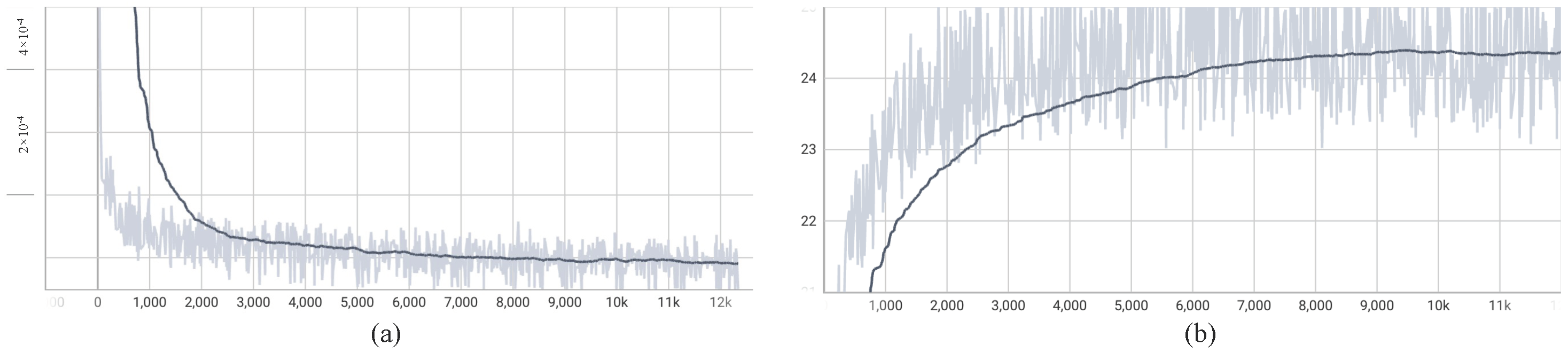
4.8. The Training Process

We trained the TSE-UNet model for a total of 60 epochs, and the curves illustrating the variations in loss and PSNR throughout the entire training procedure are shown in Figure 7. From the figure, it is evident that the convergence process of our method was stable, reaching convergence around approximately 45 epochs.

5. Conclusions

Low-cost LiDARs have lower point cloud density compared to high-cost LiDARs, which limits their perception effectiveness. To achieve better environmental perception results on low-cost LiDARs, we propose the use of TSE-UNet for sparse point cloud super-resolution. First, we project the 3D point cloud onto a 2D plane. Then, we process consecutive frames using dilated convolutional layers. We use a temporal feature aggregation convolution and a spatial attention module to extract point cloud features from consecutive frames. Using the proposed TSE-UNet model, we generate super-resolution point feature maps. Finally, by reprojecting the feature maps back into 3D space, we achieve point cloud super-resolution. Through comparative experiments, ablation experiments, visualizations, and performance testing, we demonstrate that the proposed method effectively completes the task of point cloud super-resolution. Remarkably, our approach not only achieves a PSNR of 27.52 on CARLA32-128 and 24.82 on Ruby32-128, surpassing the performance of prior methods, but also is capable of real-time operation. In the future, we plan to combine TSE-UNet with point cloud segmentation and point cloud detection tasks to promote lower-cost environmental perception for autonomous vehicles and intelligent robots.

References

1. Xu, X.; Zhang, L.; Yang, J.; Cao, C.; Wang, W.; Ran, Y.; Tan, Z.; Luo, M. A review of multi-sensor fusion slam systems based on 3D LIDAR. Remote Sens. 2022, 14, 2835. [Google Scholar] [CrossRef]
2. Chen, X.; Zhang, T.; Wang, Y.; Wang, Y.; Zhao, H. Futr3d: A unified sensor fusion framework for 3d detection. In Proceedings of the IEEE/CVF Conference on Computer Vision and Pattern Recognition, Vancouver, BC, Canada, 17–24 June 2023; pp. 172–181. [Google Scholar]
3. Aijazi, A.; Malaterre, L.; Trassoudaine, L.; Checchin, P. Systematic evaluation and characterization of 3d solid state lidar sensors for autonomous ground vehicles. Int. Arch. Photogramm. Remote Sens. Spat. Inf. Sci. 2020, 43, 199–203. [Google Scholar] [CrossRef]
4. Lin, J.; Liu, X.; Zhang, F. A decentralized framework for simultaneous calibration, localization and mapping with multiple LiDARs. In Proceedings of the 2020 IEEE/RSJ International Conference on Intelligent Robots and Systems (IROS), Las Vegas, NV, USA, 24 October 2020–24 January 2021; IEEE: Piscataway, NJ, USA, 2021; pp. 4870–4877. [Google Scholar]
5. Fei, B.; Yang, W.; Chen, W.M.; Li, Z.; Li, Y.; Ma, T.; Hu, X.; Ma, L. Comprehensive Review of Deep Learning-Based 3D Point Cloud Completion Processing and Analysis. IEEE Trans. Intell. Transp. Syst. 2022, 23, 22862–22883. [Google Scholar] [CrossRef]
6. Diab, A.; Kashef, R.; Shaker, A. Deep Learning for LiDAR Point Cloud Classification in Remote Sensing. Sensors 2022, 22, 7868. [Google Scholar] [CrossRef] [PubMed]
7. Liu, K.; Gao, Z.; Lin, F.; Chen, B.M. Fg-net: A fast and accurate framework for large-scale lidar point cloud understanding. IEEE Trans. Cybern. 2022, 53, 553–564. [Google Scholar] [CrossRef] [PubMed]
8. Chen, H.; He, X.; Qing, L.; Wu, Y.; Ren, C.; Sheriff, R.E.; Zhu, C. Real-world single image super-resolution: A brief review. Inf. Fusion 2022, 79, 124–145. [Google Scholar] [CrossRef]
9. Yue, J.; Wen, W.; Han, J.; Hsu, L.T. 3D point clouds data super resolution-aided LiDAR odometry for vehicular positioning in urban canyons. IEEE Trans. Veh. Technol. 2021, 70, 4098–4112. [Google Scholar] [CrossRef]
10. Alaba, S.Y.; Ball, J.E. A survey on deep-learning-based lidar 3d object detection for autonomous driving. Sensors 2022, 22, 9577. [Google Scholar] [CrossRef]
11. Liu, B.; Huang, H.; Su, Y.; Chen, S.; Li, Z.; Chen, E.; Tian, X. Tree species classification using ground-based LiDAR data by various point cloud deep learning methods. Remote Sens. 2022, 14, 5733. [Google Scholar] [CrossRef]
12. Bevilacqua, M.; Roumy, A.; Guillemot, C.; Alberi-Morel, M.L. Low-complexity single-image super-resolution based on nonnegative neighbor embedding. In Proceedings of the British Machine Vision Conference, BMVC 2012, Surrey, UK, 3–7 September 2012. [Google Scholar]
13. Gao, X.; Zhang, K.; Tao, D.; Li, X. Image super-resolution with sparse neighbor embedding. IEEE Trans. Image Process. 2012, 21, 3194–3205. [Google Scholar]
14. Dong, C.; Loy, C.C.; He, K.; Tang, X. Image super-resolution using deep convolutional networks. IEEE Trans. Pattern Anal. Mach. Intell. 2015, 38, 295–307. [Google Scholar] [CrossRef] [PubMed]
15. Zhang, Y.; Li, K.; Li, K.; Wang, L.; Zhong, B.; Fu, Y. Image super-resolution using very deep residual channel attention networks. In Proceedings of the European Conference on Computer Vision (ECCV), Munich, Germany, 8–14 September 2018; pp. 286–301. [Google Scholar]
16. Zhang, Y.; Li, K.; Li, K.; Zhong, B.; Fu, Y. Residual non-local attention networks for image restoration. arXiv 2019, arXiv:1903.10082. [Google Scholar]
17. Niu, B.; Wen, W.; Ren, W.; Zhang, X.; Yang, L.; Wang, S.; Zhang, K.; Cao, X.; Shen, H. Single image super-resolution via a holistic attention network. In Proceedings of the Computer Vision—ECCV 2020: 16th European Conference, Glasgow, UK, 23–28 August 2020; Part XII 16. Springer: Cham, Switzerland, 2020; pp. 191–207. [Google Scholar]
18. Dosovitskiy, A.; Beyer, L.; Kolesnikov, A.; Weissenborn, D.; Zhai, X.; Unterthiner, T.; Dehghani, M.; Minderer, M.; Heigold, G.; Gelly, S.; et al. An image is worth 16x16 words: Transformers for image recognition at scale. arXiv 2020, arXiv:2010.11929. [Google Scholar]
19. Chen, H.; Wang, Y.; Guo, T.; Xu, C.; Deng, Y.; Liu, Z.; Ma, S.; Xu, C.; Xu, C.; Gao, W. Pre-trained image processing transformer. In Proceedings of the IEEE/CVF Conference on Computer Vision and Pattern Recognition, Nashville, TN, USA, 20–25 June 2021; pp. 12299–12310. [Google Scholar]
20. Li, W.; Lu, X.; Qian, S.; Lu, J.; Zhang, X.; Jia, J. On efficient transformer-based image pre-training for low-level vision. arXiv 2021, arXiv:2112.10175. [Google Scholar]
21. Zhang, M.; Zhang, C.; Zhang, Q.; Guo, J.; Gao, X.; Zhang, J. ESSAformer: Efficient Transformer for Hyperspectral Image Super-resolution. In Proceedings of the IEEE/CVF International Conference on Computer Vision, Paris, France, 1–6 October 2023; pp. 23073–23084. [Google Scholar]
22. Ren, L.; Li, D.; Ouyang, Z.; Niu, J.; He, W. T-UNet: A Novel TC-Based Point Cloud Super-Resolution Model for Mechanical LiDAR. In Proceedings of the Collaborative Computing: Networking, Applications and Worksharing: 17th EAI International Conference, CollaborateCom 2021, Virtual Event, 16–18 October 2021; Part I 17. Springer: Cham, Switzerland, 2021; pp. 697–712. [Google Scholar]
23. Guo, M.H.; Lu, C.Z.; Liu, Z.N.; Cheng, M.M.; Hu, S.M. Visual attention network. Comput. Vis. Media 2023, 9, 733–752. [Google Scholar] [CrossRef]
24. Lin, W.; Wu, Z.; Chen, J.; Huang, J.; Jin, L. Scale-aware modulation meet transformer. In Proceedings of the IEEE/CVF International Conference on Computer Vision, Paris, France, 1–6 October 2023; pp. 6015–6026. [Google Scholar]
25. Yu, L.; Li, X.; Fu, C.W.; Cohen-Or, D.; Heng, P.A. Pu-net: Point cloud upsampling network. In Proceedings of the IEEE Conference on Computer Vision and Pattern Recognition, Salt Lake City, UT, USA, 18–23 June 2018; pp. 2790–2799. [Google Scholar]
26. Qian, Y.; Hou, J.; Kwong, S.; He, Y. PUGeo-Net: A geometry-centric network for 3D point cloud upsampling. In Proceedings of the European Conference on Computer Vision, Glasgow, UK, 23–28 August 2020; Springer: Cham, Switzerland, 2020; pp. 752–769. [Google Scholar]
27. Zhao, Y.; Hui, L.; Xie, J. Sspu-net: Self-supervised point cloud upsampling via differentiable rendering. In Proceedings of the 29th ACM International Conference on Multimedia, Virtual Event, 20–24 October 2021; pp. 2214–2223. [Google Scholar]
28. Ye, S.; Chen, D.; Han, S.; Wan, Z.; Liao, J. Meta-PU: An arbitrary-scale upsampling network for point cloud. IEEE Trans. Vis. Comput. Graph. 2021, 28, 3206–3218. [Google Scholar] [CrossRef]
29. Shan, T.; Wang, J.; Chen, F.; Szenher, P.; Englot, B. Simulation-based Lidar Super-resolution for Ground Vehicles. arXiv 2020, arXiv:2004.05242. [Google Scholar] [CrossRef]
30. Chen, Y.; Liu, S.; Wang, X. Learning continuous image representation with local implicit image function. In Proceedings of the IEEE/CVF Conference on Computer Vision and Pattern Recognition, Nashville, TN, USA, 20–25 June 2021; pp. 8628–8638. [Google Scholar]
31. Kwon, Y.; Sung, M.; Yoon, S.E. Implicit LiDAR network: LiDAR super-resolution via interpolation weight prediction. In Proceedings of the 2022 International Conference on Robotics and Automation (ICRA), Philadelphia, PA, USA, 23–27 May 2022; IEEE: Piscataway, NJ, USA, 2022; pp. 8424–8430. [Google Scholar]
32. Eskandar, G.; Sudarsan, S.; Guirguis, K.; Palaniswamy, J.; Somashekar, B.; Yang, B. HALS: A Height-Aware Lidar Super-Resolution Framework for Autonomous Driving. arXiv 2022, arXiv:2202.03901. [Google Scholar]
33. Dosovitskiy, A.; Ros, G.; Codevilla, F.; Lopez, A.; Koltun, V. CARLA: An open urban driving simulator. In Proceedings of the Conference on Robot Learning, Mountain View, CA, USA, 13–15 November 2017; pp. 1–16. [Google Scholar]
34. Ronneberger, O.; Fischer, P.; Brox, T. U-net: Convolutional networks for biomedical image segmentation. In Proceedings of the Medical Image Computing and Computer-Assisted Intervention–MICCAI 2015: 18th International Conference, Munich, Germany, 5–9 October 2015; Part III 18. Springer: Cham, Switzerland, 2015; pp. 234–241. [Google Scholar]
Figure 1. The overall pipeline of our method. RS is the LiDAR brand (RoboSense) used in this study.
Applsci 14 01510 g001
Figure 2. The images related to the CARLA32-128 dataset. (a) The scene of the CARLA simulator; (b) a bird’s-eye view of the 128-line point cloud data in CARLA32-128.
Applsci 14 01510 g002
Figure 3. The images related to the Ruby32-128 dataset. (a) The equipment we built for data acquisition; (b) a bird’s-eye view of the 128-line point cloud data in Ruby32-128.
Applsci 14 01510 g003
Figure 4. The 2D projections of 3D point clouds. From top to bottom: CARLA32, CARLA128, Ruby32, Ruby128.
Applsci 14 01510 g004
Figure 5. The architecture of TSE-UNet.
Applsci 14 01510 g005
Figure 6. The visualizations of super-resolution. The top pictures are from the CARLA32-128 dataset. The bottom pictures are from the Ruby32-128 dataset. From left to right, they are the input 32-line sparse point cloud, the ground truth of the 128-line dense point cloud, and the model’s predicted super-resolution result.
Applsci 14 01510 g006
Figure 7. (a) The depicted curve illustrates the variation in loss during the training of TSE-UNet, with the horizontal axis representing iterations and the vertical axis denoting loss values. (b) The presented curve showcases the changes in the PSNR metric during the training of TSE-UNet, with the horizontal axis indicating iterations and the vertical axis indicating PSNR values. The used dataset is Ruby32-128.
Applsci 14 01510 g007