Stable Low-Rank CP Decomposition for Compression of Convolutional Neural Networks Based on Sensitivity

Abstract

Modern convolutional neural networks (CNNs) play a crucial role in computer vision applications. The intricacy of the application scenarios and the growing dataset both significantly raise the complexity of CNNs. As a result, they are often overparameterized and have significant computational costs. One potential solution for optimizing and compressing the CNNs is to replace convolutional layers with low-rank tensor decomposition. The most suitable technique for this is Canonical Polyadic (CP) decomposition. However, there are two primary issues with CP decomposition that lead to a significant loss in accuracy. Firstly, the selection of tensor ranks for CP decomposition is an unsolved issue. Secondly, degeneracy and instability are common problems in the CP decomposition of contractional tensors, which makes fine-tuning the compressed model difficult. In this study, a novel approach was proposed for compressing CNNs by using CP decomposition. The first step involves using the sensitivity of convolutional layers to determine the tensor ranks for CP decomposition effectively. Subsequently, to address the degeneracy issue and enhance the stability of the CP decomposition, two novel techniques were incorporated: optimization with sensitivity constraints and iterative fine-tuning based on sensitivity order. Finally, the proposed method was examined on common CNN structures for image classification tasks and demonstrated that it provides stable performance and significantly fewer reductions in classification accuracy.

1. Introduction

Convolutional neural networks (CNNs) have shown advanced capabilities within a variety of domains. Nowadays, CNNs are becoming more common for use in a wide range of computer vision applications, including object recognition, image classification, and image segmentation. Nevertheless, since CNNs often have complex structures and need a lot of parameters and computational capacity, it might be challenging to apply them to computer vision tasks on edge devices with constrained resources, including embedded systems and mobile devices [1,2]. For instance, autonomous vehicles need to quickly evaluate camera frames in order to identify and avoid obstacles. The latency is increased significantly when data are sent to the cloud for inference because of queueing and network delays. For this reason, data processing needs to be performed on the device in order to be efficient during the inference. Therefore, neural networks could be compressed to reduce their size, allowing compressed versions of CNNs to operate on edge devices with limited resources.

Several popular techniques to decrease redundancy in neural network parameters include pruning [3,4], sparsification [5,6], quantization [7,8], and low-rank tensor decomposition [9,10]. Among these techniques, the tensor decomposition-based compression method is currently attracting growing interest. By decomposing the enormous weight tensors of CNNs into several compact tensor cores, tensor decomposition could result in a significant compression ratio with little accuracy reduction.

The low-rank tensor decomposition method attempts to approximate the representation of the original high-order tensors using low-rank tensors. The most prevalent approaches are Tucker decomposition [10] and Canonical Polyadic (CP) decomposition [11]. Due to its core tensors, Tucker decomposition often seems to compress less than CP decomposition. Therefore, we undertook further study into the use of low-rank CP decomposition for compressing entire CNN layers. However, CP decomposition has not been efficient for compressing CNNs due to the CP instability issue [12,13], which often impairs fine-tuning after decomposition. To overcome this problem, we propose two stable and efficient methods based on sensitivity. First, we apply sensitivity constraints for efficient optimization in CP decomposition. The sensitivity criterion reveals that traditional CP decomposition lacks robustness when subjected to minor perturbations in factor matrices, which denotes sensitivity dropping. In the optimization process, the sensitivity of the decomposition is able to be estimated and minimized to prevent degeneracy and instability in CP decomposition. Secondly, another approach to address the issue of CP decomposition instability involves the use of iterative fine-tuning, which is guided by sensitivity order. The lack of stability in CP decomposition leads to poor training results during fine-tuning, as the loss of function fails to reduce or may even be magnified when all layers are decomposed and then fine-tuned only once in the last step. Therefore, we use an iterative fine-tuning approach, performing CP decomposition and fine-tuning layer-by-layer. Furthermore, the determination of the sequence of decomposition and fine-tuning is based on the sensitivity of each layer. In general, layers with a higher sensitivity have a more significant impact on the network output and are more challenging to fine-tune. Therefore, we prioritize fine-tuning these layers for better accuracy. The experimental findings demonstrate that the aforementioned instability may be effectively addressed via sensitivity-constrained optimization and iterative fine-tuning techniques.

In the context of tensor decomposition, the issue of rank selection is another challenge worth mentioning. The significance of tensor ranks lies in their ability to balance the compression ratio and model capabilities. As a hyper-parameter, the tensor ranks play a crucial role in determining the architecture and total size of the deconstructed CNN model by quantifying the linear correlations in each dimension. Determining the most suitable rank is very complex and faces significant difficulties. Various automated rank-selection approaches have been developed to address this problem in model compression, ranging from reinforcement learning [14] to genetic algorithms [15]. In comparison to traditional manual selection methods, automatic rank-selection methods reduce human efforts for testing. However, almost all automated techniques have the following issue: as the compression ratio grows, the time required also increases because of the non-linear development in the complexity of finding a more optimal combination. To address the above issue, a novel approach is proposed to realize an efficient automatic rank-selection method based on sensitivity. Each convolutional layer’s tensor rank strongly correlates with its redundant information and compression rate. Consequently, to effectively determine the optimal ranks for tensor decomposition, a simple principle is utilized to estimate the rank: the more significant the redundancy of a layer, the lower the rank that layer requires. Therefore, we define the sensitivity of a layer as the measure of its redundancy. For layers with greater sensitivity, any perturbation will have a significant effect on the network output, indicating that it is more difficult to compress and contains less redundancy.

In this work, we leverage sensitivity to deal with two main issues with CP decomposition: rank selection and stability maintenance. Our main contributions are as follows:

• The sensitivity of each convolutional layer is computed by Hessian trace to determine the amount of redundancy of each layer, and then select the optimal ranks for CP decomposition by considering the redundancy we obtained.
• In order to overcome the CP decomposition instability problem, an efficient optimization method is developed to quantify the sensitivity of CP decomposition and add sensitivity-constrained optimization during the process.
• Another potential approach is proposed to address the problem of instability in CP decomposition by using iterative fine-tuning techniques. The layer that exhibits more sensitivity should be prioritized for compression to minimize the accuracy degradation of the compressed model.

The rest of the paper is organized as follows: In Section 2, we cover related efforts in CNN compression. A detailed description of our approach is provided in Section 3. Our experimental results and discussion are described in Section 4. Finally, we present our conclusions in Section 5.

2. Related Work

There are several methods that have been developed to make CNNs smaller, quicker, and more energy efficient. Here, we briefly discuss the related research on these CNN compression approaches.

Pruning, widely recognized as the predominant method for model compression, decreases the model size by assigning zero values to specific weight components. According to various sparsity patterns of pruning, pruning methods can be classified as either unstructured or structured. The technique of unstructured pruning, as discussed in the work of [16,17], has the potential to achieve significant compression ratios and accuracy. However, due to the unstructured feature of the sparsity pattern it produces, this strategy is unable to fully realize its theoretical acceleration on hardware systems. Structured pruning techniques, including filter [18,19] and channel [20,21] pruning, are solutions that are favorable to hardware. The performance of pruned models, however, limits the accuracy and compression ratio by the deliberately enforced structural pattern.

Sparsification is the most widely used CNN compression method. A network’s structure may be sparse at many levels, including the weight [22], filter [23], and channel [24]. A CNN model can generally be trained with sparsity-aware regularization [25] to achieve sparsity. In addition, the introduced sparsity regularization may be categorized as either structured or unstructured. Unstructured sparse models have shown excellent accuracy and compression ratio [26]. However, these models also introduce challenges such as irregular memory access and load issues of the hardware [27]. Structured sparse models are sometimes considered to be more suitable for hardware implementation due to their inherent architecture. However, it is worth noting that these models often exhibit worse compression ratios and accuracy compared to their unstructured counterparts [28].

Quantization is a compression technique commonly used in CNN implementation in hardware, particularly for specialized CNN chips [29]. It utilizes a restricted number of bits for representing weight and activation [30,31]. The choice of precision often depends on the available resource allocation and the desired level of accuracy. To achieve extremely low storage and computational costs, 1-bit weight has been proposed in [32] as a highly aggressive quantization approach.

Tensor decomposition is a widely used technique in tensor theory, with the purpose of achieving compact representation of massive high-dimensional tensor-format data. Beginning with Tucker decomposition [10], numerous tensor decomposition techniques have been developed to compress CNNs by decomposing the original tensors into compact core tensors. In the studies of [33,34,35], decomposition methods of the tensor train (TT) [35], tensor ring (TR) [33], and hierarchical Tucker (HT) [34] have been utilized to obtain simple RNN architectures, resulting in a significant decrease in model parameters. The most recent study [36] introduces a low-rank Tucker-CP decomposition method. This method aims to enhance the approximation of weight tensors in convolutional layers, enabling effective CNN compression while preserving high accuracy.

3. The Proposed Method

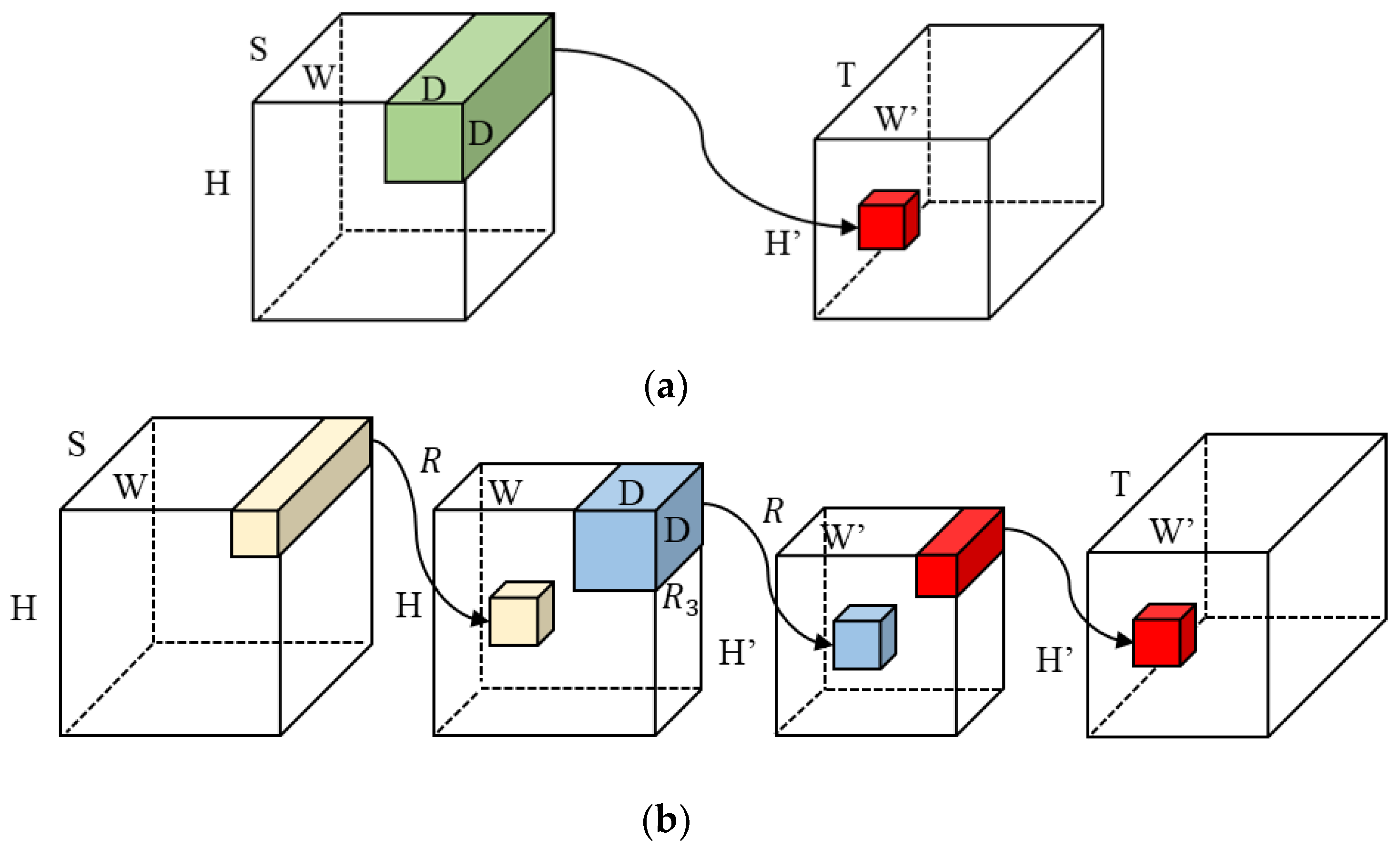
3.1. CP Decomposition for Convolutional Layers

In the process of CP decomposition, a tensor is decomposed by CP into a linear combination of rank-one tensors. We focus on the three-way tensor and consider that a tensor $\mathcal{T}$ is denoted as:

$$\begin{array}{c}\mathcal{T}=⟦\mathrm{A},\mathrm{B},\mathrm{C}⟧,\end{array}$$

(1)

where $\mathrm{A}$, $\mathrm{B}$, and $\mathrm{C}$ denote factor matrices of tensor $\mathcal{T}$. The notation $⟦\dots ⟧$ denotes that:

$$\begin{array}{c}\mathcal{T}={\displaystyle \sum _{r=1}^R}{\mathrm{a}}_{\mathrm{r}}\otimes {\mathrm{b}}_{\mathrm{r}}\otimes {\mathrm{c}}_{\mathrm{r}},\end{array}$$

(2)

where $\otimes$ is the outer product of the tensors. The decomposition of the tensor $\mathcal{T}$ into its R components is shown in Equation (2). The tensor rank is the overall amount of components in the decomposed tensor, denoted by R. The rank R is a determining factor in the extent of weight reduction in a convolution layer. Specifically, a lower value of R corresponds to a greater weight decrease. $\left\{{\mathrm{a}}_{\mathrm{r}}\right\}$, $\left\{{\mathrm{b}}_{\mathrm{r}}\right\}$, and $\left\{{\mathrm{c}}_{\mathrm{r}}\right\}$ denote the columns of factor matrices $\mathrm{A}$, $\mathrm{B}$, and $\mathrm{C}$, respectively.

Then, we focus on the tensor of the convolution layer. Convolution layers in CNNs typically transform an input tensor $\mathcal{X}$, with dimensions $S\times W\times H$, into an output tensor $\mathcal{Y}$, with dimensions $T\times W^{\prime }\times H^{\prime }$. This transformation is achieved by utilizing a four-dimensional kernel tensor $\mathcal{K}$, with dimensions $T\times S\times D\times D$. We assume that kernel tensors are square-shaped and have an odd dimension $D$:

$$\begin{array}{c}{\mathcal{Y}}_{t,w^{\prime },h^{\prime }}={\displaystyle \sum _{s=1}^S}{\displaystyle \sum _{j=1}^D}{\displaystyle \sum _{i=1}^D}{\mathcal{K}}_{t,s,j,i}{\mathcal{X}}_{s,w_j,h_i}.\end{array}$$

(3)

Now, the current problem involves the approximation of the tensor $\mathcal{K}$ using CP decomposition with rank $R$. This is illustrated by Equation (4). The spatial dimensions of tensor $\mathcal{K}$ are not decomposed due to their relatively modest size, such as 3 × 3 or 5 × 5:

$$\begin{array}{c}{\mathcal{K}}_{t,s,j,i}={\displaystyle \sum _{r=1}^R}{\mathrm{U}}_{r,s}^{\left(1\right)}{\mathcal{U}}_{r,j,i}^{\left(2\right)}{\mathrm{U}}_{t,r}^{\left(3\right)},\end{array}$$

(4)

where ${\mathrm{U}}_{r,s}^{\left(1\right)}$, ${\mathcal{U}}_{r,j,i}^{\left(2\right)}$, and ${\mathrm{U}}_{t,r}^{\left(3\right)}$ are the three tensors with sizes $R\times S$, $R\times D\times D$, and $T\times R$, respectively.

By substituting Equation (4) into Equation (3), we obtain an approximate method to calculate the convolution (3):

$$\begin{array}{c}{\mathcal{Y}}_{t,w^{\prime },h^{\prime }}={\displaystyle \sum _{r=1}^R}{\mathrm{U}}_{t,r}^{\left(3\right)}\left({\displaystyle \sum _{j=1}^D}{\displaystyle \sum _{i=1}^D}{\mathcal{U}}_{r,j,i}^{\left(2\right)}\left({\displaystyle \sum _{s=1}^S}{\mathrm{U}}_{r,s}^{\left(1\right)}{\mathcal{X}}_{s,w_j,h_i}\right)\right).\end{array}$$

(5)

As illustrated in Figure 1, Equation (5) denotes that the output tensor $\mathcal{Y}$ is derived by a series of distinct and compact convolutions applied to the input tensor X:

$$\begin{array}{c}{\mathcal{Z}}_{r,w,h}={\displaystyle \sum _{s=1}^S}{\mathrm{U}}_{r,s}^{\left(1\right)}{\mathcal{X}}_{s,w,h},\end{array}$$

(6)

$$\begin{array}{c}{\mathcal{Z}}_{r,w^{\prime },h^{\prime }}^{\prime }={\displaystyle \sum _{j=1}^D}{\displaystyle \sum _{i=1}^D}{\mathcal{U}}_{r,j,i}^{\left(2\right)}{\mathcal{Z}}_{t,w_j,h_i},\end{array}$$

(7)

$$\begin{array}{c}{\mathcal{Y}}_{t,w^{\prime },h^{\prime }}={\displaystyle \sum _{r=1}^R}{\mathrm{U}}_{t,r}^{\left(3\right)}{\mathcal{Z}}_{r,w^{\prime },h^{\prime }}^{\prime },\end{array}$$

(8)

where ${\mathcal{Z}}_{r,w,h}$ and ${\mathcal{Z}}_{r,w^{\prime },h^{\prime }}^{\prime }$ are intermediate tensors with dimensions $R\times W\times H$ and $R\times W^{\prime }\times H^{\prime }$, respectively.

3.2. Rank Selection Based on Sensitivity

The purpose of rank selection is significant in CP decomposition. Insufficient compression would result from an excessively high rank, while too low a rank would lead to a significant decrease in accuracy that cannot be compensated for by fine-tuning. However, a definitive approach for determining the optimal tensor rank does not currently exist. Indeed, the computational problem of finding the rank is NP-hard [37]. Therefore, an essential idea is used for estimating the rank: the relationship between redundancy and compression rate is inversely proportional, so the relationship between redundancy and rank is directly proportional. Specifically, as the redundancy of a layer increases, the required rank of the layer decreases. To estimate the redundancy of each layer, a layer’s sensitivity can be defined as its responsiveness to redundancy through compression. If a layer has a high level of sensitivity, it would be unfavorable to put the rank at a low value, and vice versa.

We propose the use of a sensitivity-based rank-selection method. The sensitivity can be quantified by calculating the average of the Hessian trace. More specifically, the Hessian can be efficiently estimated using randomized numerical linear algebra approaches, such as Hutchinson’s approach [38]. Significantly, this method just needs the calculation of the Hessian on an input vector that is generated at random. The computational cost is equivalent to that of back-propagating the gradient. A similar method has been proposed by [8] in terms of quantization.

Here, our focus is on the trace of a matrix $H\in R^{d\times d}$. Next, with a random vector $z\in R^d$ whose component is i.i.d. sampled Gaussian distribution, we can obtain:

$$\begin{array}{c}\mathrm{Tr}\left(H\right)=\mathrm{Tr}\left(HI\right)=\mathrm{Tr}\left(H\mathbb{E}\left[z{z}^T\right]\right)=E\left[\mathrm{Tr}\left(Hz{z}^T\right)\right]=E\left[z^{T}Hz\right],\end{array}$$

(9)

where $I$ denotes the identity matrix. Then the Hutchinson algorithm [4] can be utilized to compute the Hessian trace:

$$\begin{array}{c}\mathrm{Tr}\left(H\right)\approx \frac{1}{m}{\displaystyle \sum _{i=1}^m}{z}_i^{T}H{z}_i=T{r}_{Est}\left(H\right).\end{array}$$

(10)

Finally, the rank of each layer is calculated in proportion to its sensitivity. By calculating and comparing the Hessian trace of each layer in the CNN, the ratio is able to measure the relative sensitivity and guide the selection of the rank for each layer. However, since we only know the ratio, the average rank of all layers must be selected arbitrarily.

3.3. Sensitivity-Constrained Optimization in CP Decomposition

Tensor decomposition can be considered as an optimization problem, i.e., minimizing the difference between the decomposed tensor and the original tensor. In the optimization process of CP decomposition, there may be some problems. For instance, it is common to observe that two rank-one tensors with relatively high Frobenius norms cancel each other out when applying optimization algorithms to low-rank decomposition with nonunique CP decomposition [39]. This degeneracy is a common phenomenon in most CP decompositions of the convolutional layer. The presence of degeneracy often leads to instability problems when retraining a neural network with a CP format [12,13]. In particular, it impairs the ability of a model to complete fine-tuning and preserve network stability.

Therefore, a stable method is introduced from the work of [40] to perform sensitivity-based CP decomposition. To obtain a more stable decomposition, [40] proposed a correction to the decomposition optimization with less sensitivity. The study revealed that sensitivity might be used as a potential metric to evaluate the level of degeneracy in the CP decomposition. Consequently, we intend to quantify the sensitivity and perform sensitivity-constrained optimization in CP decomposition.

When decomposing the tensor $\mathcal{K}$ of convolutional kernels using CP decomposition, as previously mentioned, the kernel $\mathcal{K}$ is considered an order-3 tensor $\mathcal{K}=⟦\mathrm{A},\mathrm{B},\mathrm{C}⟧$ with dimensions $T\times S\times D^2$. Due to the spatial dimensions of the tensor $\mathcal{K}$ being so small, it is not necessary to decompose them. Subsequently, the sensitivity is defined as:

$$\begin{array}{c}S\left(\mathcal{K}\right)=\underset{{\sigma }^2\to 0}{\mathrm{l}\mathrm{i}\mathrm{m}}\frac{1}{R{\sigma }^2}E\left\{\parallel \mathcal{K}-\left[\right[\mathrm{A}+\mathsf{\delta }\mathrm{A},\mathrm{B}+\mathsf{\delta }\mathrm{B},\mathrm{C}+\mathsf{\delta }\mathrm{C}\left]\right]{\parallel }_{\mathrm{F}}^2\right\}\end{array}$$

(11)

where $\delta \mathrm{A}$, $\delta \mathrm{B}$, and $\delta \mathrm{C}$ denote elements with i.i.d. Gaussian distribution $N(0,{\sigma }^2)$.

The sensitivity could be quantified by calculating the expectation ($E\{·\}$) of the normalized squared Frobenius norm of the difference. Essentially, the sensitivity of the tensor $\mathcal{K}$ is a metric that is relative to perturbations in individual factor matrices. Additionally, CP decomposition with great sensitivity is often ineffective.

Upon performing a simple calculation, the expectation ($E\{·\}$) in Equation (11) may be represented in the following form:

$$\begin{array}{c}\begin{array}{c}E\left\{\parallel \mathcal{K}-⟦\mathrm{A}+\delta \mathrm{A},\mathrm{B}+\delta \mathrm{B},\mathrm{C}+\delta \mathrm{C}⟧{\parallel }_F^2\right\}\hfill \\ \hspace{1em}\hspace{1em}=E\left\{\parallel ⟦\delta \mathrm{A},\mathrm{B},\mathrm{C}⟧{\parallel }_F^2\right\}+E\{\parallel ⟦\mathrm{A},\delta \mathrm{B},\mathrm{C}⟧{\parallel }_F^2\}+E\{\parallel ⟦\mathrm{A},\mathrm{B},\delta \mathrm{C}⟧{\parallel }_F^2\}\hfill \\ \hspace{1em}\hspace{1em}=R{\sigma }^2\mathrm{tr}\left(\left({\mathrm{C}}^T\mathrm{C}\right)⊛\left({\mathrm{B}}^T\mathrm{B}\right)\right)+R{\sigma }^2\mathrm{tr}\left(\left({\mathrm{C}}^T\mathrm{C}\right)⊛\left({\mathrm{A}}^T\mathrm{A}\right)\right)\hfill \\ \hspace{1em}\hspace{1em}\hspace{1em}+R{\sigma }^2\mathrm{tr}\left(\left({\mathrm{B}}^T\mathrm{B}\right)⊛\left({\mathrm{A}}^T\mathrm{A}\right)\right)\hfill \end{array},\end{array}$$

(12)

where $⊛$ is the Hadamard element-wise product, while “tr” refers to the trace of a matrix. Subsequently, we substitute this equation into the aforementioned Equation (11) to obtain the compact representation of sensitivity:

$$\begin{array}{c}\begin{array}{cc}S\left(\mathcal{K}\right)& =tr\left(\left({\mathrm{A}}^T\mathrm{A}\right)⊛\left({\mathrm{B}}^T\mathrm{B}\right)+\left({\mathrm{B}}^T\mathrm{B}\right)⊛\left({\mathrm{C}}^T\mathrm{C}\right)+\left({\mathrm{A}}^T\mathrm{A}\right)⊛\left({\mathrm{C}}^T\mathrm{C}\right)\right)\hfill \\ & ={\displaystyle \sum _{r=1}^R}{\parallel {\mathrm{a}}_r\parallel }^2{\parallel {\mathrm{b}}_r\parallel }^2+{{\parallel {\mathrm{a}}_r\parallel }^2\parallel {\mathrm{c}}_r\parallel }^2+{\parallel {\mathrm{b}}_r\parallel }^2{\parallel {\mathrm{c}}_r\parallel }^2\hfill \end{array}.\end{array}$$

(13)

Next, our goal is to minimize the sensitivity while maintaining the error of optimization:

$$\begin{array}{c}\begin{array}{cc}\underset{\left\{\mathrm{A},\mathrm{B},\mathrm{C}\right\}}{min}& \mathrm{S}\left(⟦\mathrm{A},\mathrm{B},\mathrm{C}⟧\right)\\ \mathrm{s}.\mathrm{t}.& \parallel \mathcal{K}-⟦\mathrm{A},\mathrm{B},\mathrm{C}⟧{\parallel }_F^2\le {\delta }^2.\end{array}\end{array}$$

(14)

The constraint ${\delta }^2$ can be utilized to define the approximation errors of optimization in the decomposition. Then, we can update the tensor $\mathcal{K}$ with a lower sensitivity to enhance the convergence of CP decomposition.

Iterative updating equations have been used for the aforementioned optimization issue (14). With $\mathrm{B}$ and $\mathrm{C}$ remaining fixed, the objective of optimization is modified to update $\mathrm{A}$ as follows:

$$\begin{array}{c}\begin{array}{cc}\underset{\mathrm{A}}{min}& \mathrm{tr}\left\{\left({\mathrm{A}}^T\mathrm{A}\right)⊛\left({\mathrm{B}}^T\mathrm{B}+{\mathrm{C}}^T\mathrm{C}\right)\right\}\\ \mathrm{s}.\mathrm{t}.& {\parallel {\mathrm{K}}_{\left(1\right)}-\mathrm{A}{\left(\mathrm{C}\odot \mathrm{B}\right)}^T\parallel }_F^2\le {\delta }^2,\end{array}\end{array}$$

(15)

where ${\mathrm{K}}_{\left(1\right)}$ is mode-1 unfolding of the kernel tensor $\mathcal{K}$, and $\odot$ is Kronecker products. The optimization issue (15) can be regarded as a regression problem with constraints. It may be efficiently addressed using a closed-form solution using the technique from [41].

3.4. Iterative Fine-Tuning Based on Sensitivity

CP decomposition often leads to a drop in the accuracy of CNNs due to the optimization errors of decomposition. To restore the lost accuracy, fine-tuning is a necessary process. Nevertheless, the application of CP decomposition to each layer with one-time fine-tuning has not been effective because of its inherent instability [11]. Therefore, after decomposing each layer, we fine-tune the entire model iteratively to overcome the instability and prevent the errors from becoming unrecoverable.

The arrangement of convolutional layers plays a crucial role in iterative CP decomposition and fine-tuning. In general, the performance of a network using iterative decomposition and fine-tuning is influenced by the varying sensitivity information of each individual layer. Therefore, we introduce sensitivity to determine the sequence of decomposition and fine-tuning for each convolutional layer. Specifically, layers with higher sensitivity have a greater impact on the output of CNNs, and it is more difficult to recover their accuracy by fine-tuning after decomposition, so we prioritize compressing convolutional layers with higher sensitivity in the original network, and then iterate until the whole model is compressed. By using this iterative fine-tuning approach that considers sensitivity, we anticipate that the overall error of the compressed model will be effectively controlled, preventing it from reaching an unrecoverable magnitude.

As illustrated in Figure 2, the procedure of our method to compress the original model includes four essential steps:

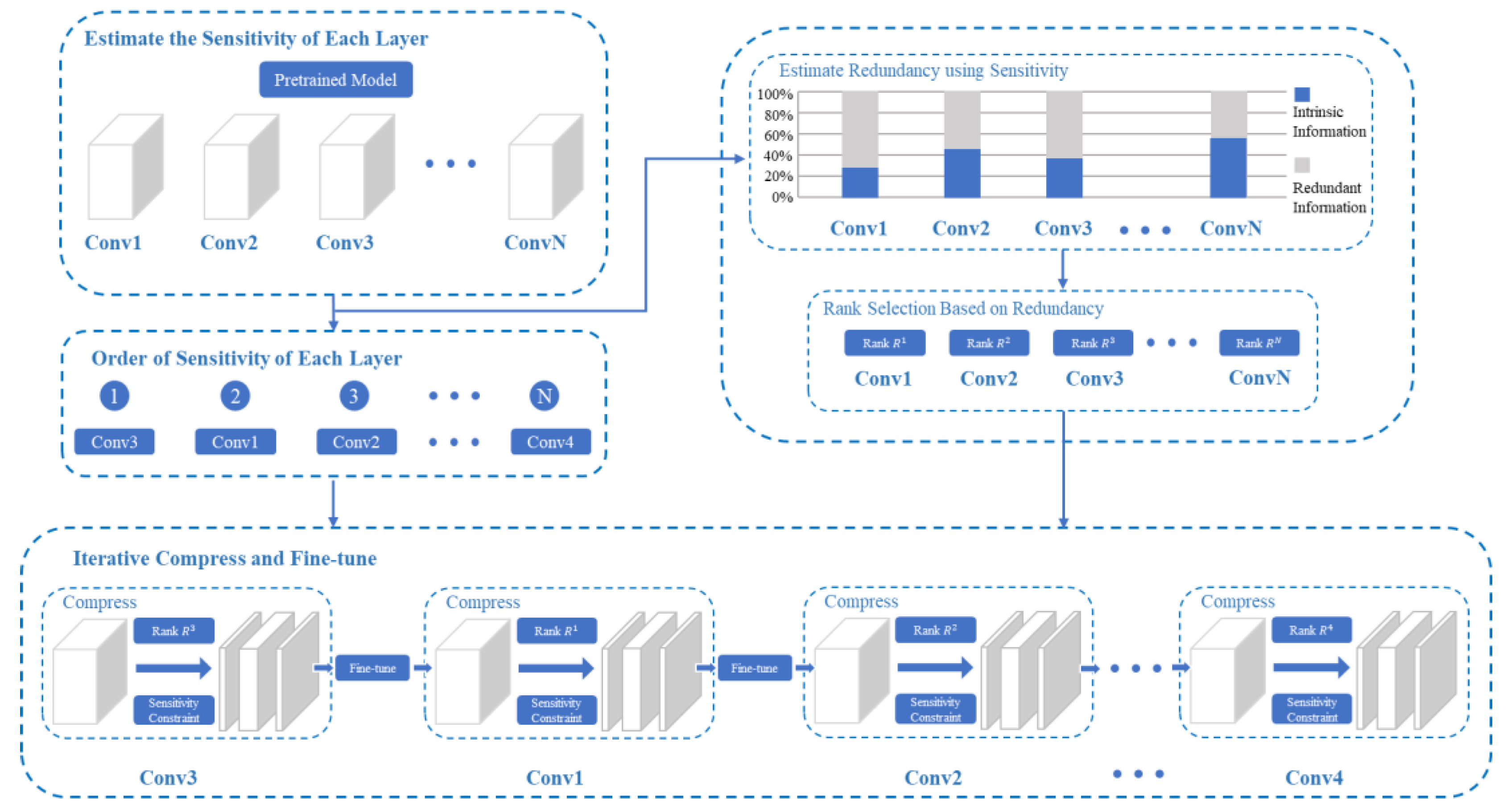
• Estimating the sensitivity of each layer in the original model.
• Sorting each network layer according to the order of the sensitivity information content of each network layer from large to small.
• Determining the rank of each layer according to its sensitivity and an average rank we set in advance.
• Iterative compressing and fine-tuning based on the sensitivity of each layer. The sorting results obtained from the second step and the rank obtained from the third step are used to iteratively compress and fine-tune the network layer-by-layer.

4. Experimental Results

To prove the effectiveness of the proposed approach, we tested several CNN models in popular image classification tasks. The proposed approach has been rigorously evaluated on several different size datasets (ImageNet [42], CIFAR-10, and CIFAR-100 [43]) and well-known CNN architectures VGG [44] and Resnet [45]. With the CIFAR-10 dataset, we trained the ResNet-20 and ResNet-32 neural networks to evaluate our method. The ResNet-20 and ResNet-32 models were trained following the guidelines given by [45]. For testing our approach on ImageNet, we implemented ResNet-18 and ResNet-50 neural networks, and the pretrained models utilized in this study were derived from the Torchvision package of PyTorch.

4.1. Experimental Results on CIFAR-10

Table 1. Comparison with various tensor decomposition methods for ResNet-20 and ResNet-32 on CIFAR-10 dataset.

Model	Method	Compression Method	Top-1 Acc (%)	Compression Ratio
Resnet-20	Standard Tucker [10]	Tucker	−3.84	2.6×
	Standard Tensor Train [47]	Tensor Train	−4.55	5.4×
	Standard Tensor Ring [48]	Tensor Ring	−3.75	5.4×
	PSTR-S [46]	Tensor Ring	−0.45	2.5×
	PSTR-M [46]	Tensor Ring	−2.75	6.8×
	Ours	CP	−0.31	2.6×
	Ours	CP	−1.82	6.8×
Resnet-32	Standard Tucker [10]	Tucker	−4.79	5.1×
	Standard Tensor Train [47]	Tensor Train	−4.19	4.8×
	Standard Tensor Ring [48]	Tensor Ring	−1.89	5.1×
	PSTR-S [46]	Tensor Ring	−1.05	2.7×
	PSTR-M [46]	Tensor Ring	−1.89	5.8×
	Ours	CP	−0.45	2.8×
	Ours	CP	−1.31	5.8×

illustrates the test results on the CIFAR-10 dataset. Specifically, using the ResNet-20 model, we achieved superior performance compared to the traditional Tucker decomposition technique, with a 3.53% increase in accuracy, while maintaining the same compression ratio of 2.6×. In addition, our method demonstrates a considerable performance improvement (0.93% higher accuracy) when compared to the Tensor Ring tensor technique [46], while maintaining the same compression ratio of 6.8×. Regarding ResNet-32, our approach outperforms the existing methods. When compared to PSTR-S, our method’s trained model yields a 0.6% increase in accuracy while maintaining a better compression ratio of 2.8×. Furthermore, with the same compression ratio of 5.8×, we achieved a 0.58% increase in accuracy.

4.2. Experimental Results on CIFAR-100

The results of the test for the CIFAR-100 dataset are shown in

Table 2. Comparison with various tensor decomposition methods for ResNet-20 and ResNet-32 on CIFAR-100 dataset.

Model	Method	Compression Method	Top-1 Acc (%)	Compression Ratio
Resnet-20	Standard Tucker [10]	Tucker	−7.87	2.5×
	Standard Tensor Train [47]	Tensor Train	−3.76	5.6×
	Standard Tensor Ring [48]	Tensor Ring	−1.85	4.7×
	PSTR-S [46]	Tensor Ring	+0.73	2.3×
	PSTR-M [46]	Tensor Ring	−1.78	4.7×
	Ours	CP	+1.05	2.6×
	Ours	CP	−1.32	4.7×
Resnet-32	Standard Tucker [10]	Tucker	−9.07	2.5×
	Standard Tensor Train [47]	Tensor Train	−5.20	4.6×
	Standard Tensor Ring [48]	Tensor Ring	−1.40	4.8×
	PSTR-S [46]	Tensor Ring	−0.05	2.4×
	PSTR-M [46]	Tensor Ring	−1.33	5.2×
	Ours	CP	−0.25	2.5×
	Ours	CP	−0.81	5.2×

. For ResNet-20, we obtain an 8.92% increase in accuracy compared to the Tucker decomposition method, while also achieving a higher compression ratio. When compared to the PSTR-S [46], our approach achieves 0.32% better accuracy and a 0.3× higher compression ratio. In comparison to the original uncompressed model, this performance is even better by 1.05%. Even when the desired compression ratio is increased to 4.7×, our approach continues to surpass the PSTR-M [46] with 0.46% better accuracy. For ResNet-32, the proposed approach obtains an accuracy increase of 8.82% and 0.2%, respectively, over standard Tucker decomposition and PSTR-S [46]. Furthermore, with the same 5.2× compression ratio, our method achieves a 0.52% increase in accuracy compared to PSTR-M [46].

4.3. Experimental Results on ImageNet

We also examine the proposed approach using ImageNet to compress the VGG-16, ResNet-18, and ResNet-50 models. Table 3 shows a comparative analysis of our method’s performance against existing tensor decomposition techniques, and other compression strategies like pruning and Low-Rank Matrix decomposition. As these studies focus on providing a decrease in FLOPs, rather than the compression ratio, we also include the FLOPs reduction achieved using tensor decomposition.

We used our method to compress the VGG-16 neural network, which is the largest deep neural network examined in this paper. The results in Table 3 show that our method yielded higher accuracy at a nearly similar drop in FLOPs as HT-2 [7]. The rest of the methods lead to worse compression results. It is noteworthy that our approach achieved the best Top-5 accuracy in the whole set of methods analyzed.

When comparing ResNet-18, our technique achieves better accuracy than MUSCO [49] and TRP [50] by 0.14% and 2.18%, respectively, while maintaining an almost similar reduction ratio of FLOPs (4.6×). Our models achieve much higher accuracy while reducing FLOPs more effectively compared to existing compression methods that result in noticeable accuracy loss. Specifically, our model achieves a reduction of 2.47× in FLOPs and suffers a mere 0.16% decrease in accuracy compared to the original model.

ResNet-50 is a more extensive and more complex model in comparison to ResNet-18. Table 3 demonstrates that our method shows superior performance across nearly all metrics compared to the other pruning approaches. Concerning the decomposition-based methods, which include Tucker decomposition and low-rank matrix decomposition, it is evident that all the mentioned decomposition-based approaches yielded inferior results in comparison to our approach. Furthermore, with a compression of 2.97× FLOPs, our compressed model achieves a Top-5 accuracy loss 0.51% less than the uncompressed model.

Table 3. Comparison with various compression methods for VGG-16, ResNet-18, and ResNet-50 on ImageNet dataset.

Model	Method	Compression Method	Top-5 Acc (%)	FLOPs Reduction
VGG-16	AutoPruner [51]	Pruning	−1.49	3.79×
	Standard Tucker [10]	Tucker	−0.50	4.93×
	HT-2 [52]	Tucker	−0.65	5.26×
	Ours	CP	−0.38	5.26×
Resnet-18	FPGM [53]	Pruning	−0.55	1.72×
	DSA [54]	Pruning	−0.73	1.72×
	DACP [20]	Pruning	−1.48	1.89×
	Standard Tucker [10]	Tucker	−1.55	2.25×
	MUSCO [49]	Tucker	−0.30	2.42×
	TRP [50]	Low-Rank Matrix	−2.34	2.60×
	Ours	CP	−0.16	2.61×
Resnet-50	TRP [50]	Low-Rank Matrix	−0.80	1.80×
	Standard Tucker [10]	Tucker	−1.75	2.04×
	AKECP [55]	Pruning	−2.30	2.62×
	HRANK [18]	Pruning	−1.86	2.64×
	HT-2 [52]	Tucker	−0.71	2.85×
	AutoPruner [51]	Pruning	−1.62	2.94×
	Ours	CP	−0.51	2.97×

Table 3. Comparison with various compression methods for VGG-16, ResNet-18, and ResNet-50 on ImageNet dataset.

Model	Method	Compression Method	Top-5 Acc (%)	FLOPs Reduction
VGG-16	AutoPruner [51]	Pruning	−1.49	3.79×
	Standard Tucker [10]	Tucker	−0.50	4.93×
	HT-2 [52]	Tucker	−0.65	5.26×
	Ours	CP	−0.38	5.26×
Resnet-18	FPGM [53]	Pruning	−0.55	1.72×
	DSA [54]	Pruning	−0.73	1.72×
	DACP [20]	Pruning	−1.48	1.89×
	Standard Tucker [10]	Tucker	−1.55	2.25×
	MUSCO [49]	Tucker	−0.30	2.42×
	TRP [50]	Low-Rank Matrix	−2.34	2.60×
	Ours	CP	−0.16	2.61×
Resnet-50	TRP [50]	Low-Rank Matrix	−0.80	1.80×
	Standard Tucker [10]	Tucker	−1.75	2.04×
	AKECP [55]	Pruning	−2.30	2.62×
	HRANK [18]	Pruning	−1.86	2.64×
	HT-2 [52]	Tucker	−0.71	2.85×
	AutoPruner [51]	Pruning	−1.62	2.94×
	Ours	CP	−0.51	2.97×

4.4. Discussion

To obtain a thorough comprehension of the impact of the proposed approach, we also examine the training process for compressing ResNet-18 on the ImageNet dataset.

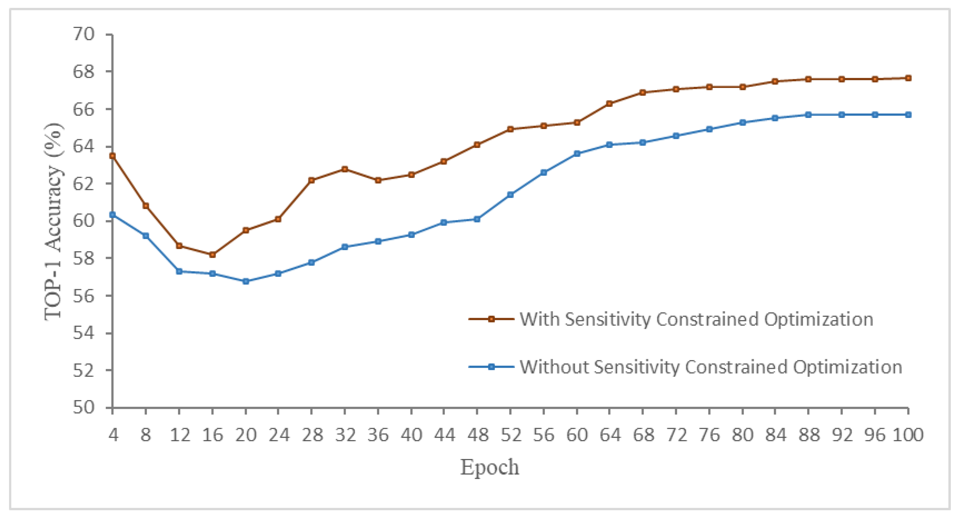
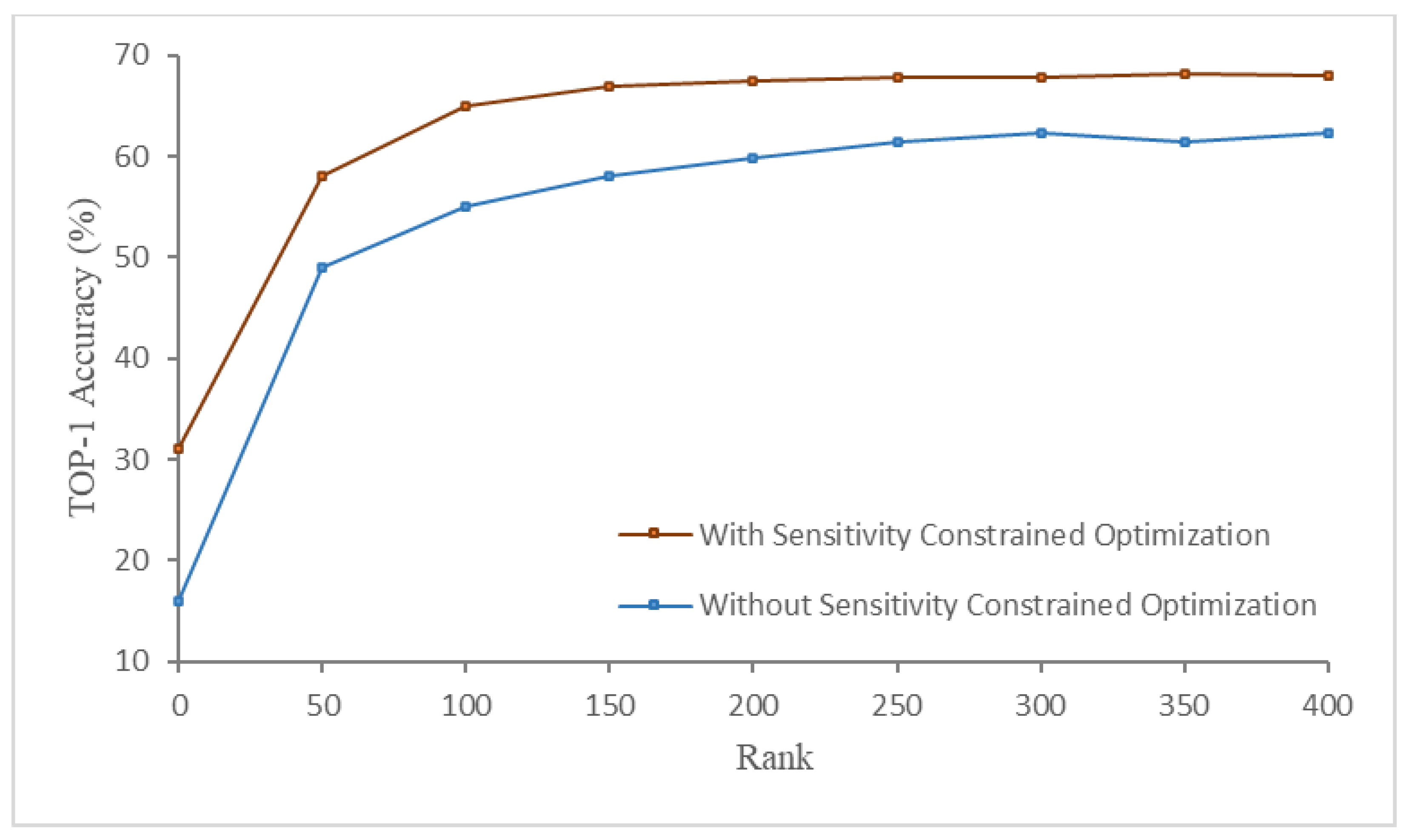
4.4.1. Sensitivity-Constrained Optimization

To evaluate the effect of the sensitivity-constrained optimization, we implemented some comparative experiments. Figure 3 demonstrates an illustrative example, in which only CP decomposes a single convolutional layer 1 of block 4 in ResNet-18. Our results demonstrate that we obtain superior accuracy compared to standard CP (without sensitivity-constrained optimization) with the same epoch of fine-tuning. Figure 4 demonstrates another illustrative example of the effectiveness of our method. It is crucial to note that the compressed network, which utilizes standard CP (without sensitivity-constrained optimization), fails to obtain the same Top-1 accuracy of the original network, even when the rank is set at 400 and fine-tuning is applied. Nevertheless, by using sensitivity-constrained optimization, the performance significantly improves and achieves the level of original accuracy. Even the model with a rank of 100 produces comparatively excellent results, with less than 2% accuracy loss.

4.4.2. Iterative Fine-Tuning Based on Sensitivity Order

To investigate the effects of iterative fine-tuning based on sensitivity, we performed several ablation studies with ResNet-18 compression models on ImageNet. Other models and datasets can provide similar results.

We start with one-shot fine-tuning, which means only fine-tuning once after all convolutional layers have been CP decomposed. We label this as CP-one-shot in

Table 4. Ablation results in iterative fine-tuning based on sensitivity order.

Model	Method	Top-1 Acc (%)	Top-5 Acc (%)	FLOPs Reduction
Resnet-18	CP-one-shot	−4.09	−2.57	2.61×
	CP-random	−2.23	−1.31	2.61×
	Ours	−1.28	−0.16	2.61×
Resnet-50	CP-one-shot	−6.27	−3.62	2.97×
	CP-random	−4.07	−1.86	2.97×
	Ours	−1.34	−0.51	2.97×

. Meanwhile, to validate the performance of our approach, which uses sensitivity order to guide the process of iterative fine-tuning, we also conduct tests for iterative fine-tuning with random order, denoted as CP-random in Table 4.

For a fair comparison, the other parameters for these different fine-tuning strategies remain the same, such as tensor rank in each individual layer and sensitivity-constrained optimization in CP decomposition. According to the results, the CP-one-shot strategy presents the lowest Top-1 and Top-5 accuracy compared with CP-random and our method in the same FLOPs reduction.

On the contrary, our approach yields optimal accuracy for the ResNet-18 models. This indicates that sensitivity-based iterative fine-tuning combined with CP decomposition is the most effective strategy for restoring the loss of accuracy.

5. Conclusions

In this paper, we propose a novel approach for CNN decomposition based on sensitivity. The approach involves decomposing a network using CP decomposition, optimizing the decomposition with a sensitivity constraint, and recovering the network by iterative fine-tuning depending on the sensitivity order of each layer. The results of the experiments conducted on three popular datasets with different large-scale CNNs clearly show that our approach outperforms the existing methods, including the most common pruning approaches and other low-rank compression approaches. Therefore, we conclude that our method is quite competitive with other compression strategies that are considered for CNN compression on a large scale.

There remain some limitations and much work to be further researched. Firstly, the sensitivity metric used for rank selection is a heuristic metric and lacks theoretical analysis. Figuring out the ranks with a better metric will be a key issue in further research. Secondly, since the process of iterative fine-tuning needs too much computation, how to enhance the computational efficiency is another important problem. Third, although our method achieved better experimental results compared to the state-of-the-art compression method, its advantages are not obvious, and further improvement is needed. Finally, this work has only focused on the compression of convolution layers, and fully connected layers also need to be considered.

References

1. Jiang, P.; Zhang, Z.; Dong, Z.; Yang, Y.; Pan, Z.; Deng, J. Axial and radial electromagnetic-vibration characteristics of converter transformer windings under current harmonics. High Volt. 2023, 8, 477–491. [Google Scholar] [CrossRef]
2. Zhao, H.; Zhang, Z.; Yang, Y.; Xiao, J.; Chen, J. A Dynamic Monitoring Method of Temperature Distribution for Cable Joints Based on Thermal Knowledge and Conditional Generative Adversarial Network. IEEE Trans. Instrum. Meas. 2023, 72, 4507014. [Google Scholar] [CrossRef]
3. Fang, G.; Ma, X.; Song, M.; Mi, M.B.; Wang, X. Depgraph: Towards any structural pruning. In Proceedings of the IEEE/CVF Conference on Computer Vision and Pattern Recognition, Vancouver, BC, Canada, 17–24 June 2023; pp. 16091–16101. [Google Scholar]
4. Liu, Y.; Wu, D.; Zhou, W.; Fan, K.; Zhou, Z. EACP: An effective automatic channel pruning for neural networks. Neurocomputing 2023, 526, 131–142. [Google Scholar] [CrossRef]
5. Molchanov, D.; Ashukha, A.; Vetrov, D. Variational Dropout Sparsifies Deep Neural Networks. In Proceedings of the 34th International Conference on Machine Learning, Sydney, NSW, Australia, 6–11 August 2017; Precup, D., Teh, Y.W., Eds.; 2017; Volume 70, pp. 2498–2507. [Google Scholar]
6. Han, S.; Pool, J.; Tran, J.; Dally, W. Learning Both Weights and Connections for Efficient Neural Network. In Proceedings of the Advances in Neural Information Processing Systems; Curran Associates, Inc.: Red Hook, NY, USA, 2015; Volume 28, pp. 1135–1143. [Google Scholar]
7. Rokh, B.; Azarpeyvand, A.; Khanteymoori, A. A comprehensive survey on model quantization for deep neural networks in image classification. ACM Trans. Intell. Syst. Technol. 2023, 14, 1–50. [Google Scholar]
8. Dong, Z.; Yao, Z.; Arfeen, D.; Gholami, A.; Mahoney, M.W.; Keutzer, K. HAWQ-V2: Hessian Aware Trace-Weighted Quantization of Neural Networks. In Proceedings of the Advances in Neural Information Processing Systems; Larochelle, H., Ranzato, M., Hadsell, R., Balcan, M.F., Lin, H., Eds.; Curran Associates, Inc.: Red Hook, NY, USA, 2020; Volume 33, pp. 18518–18529. [Google Scholar]
9. Kossaifi, J.; Toisoul, A.; Bulat, A.; Panagakis, Y.; Hospedales, T.M.; Pantic, M. Factorized Higher-Order CNNs With an Application to Spatio-Temporal Emotion Estimation. In Proceedings of the IEEE/CVF Conference on Computer Vision and Pattern Recognition (CVPR), Seattle, WA, USA, 13–19 June 2020; pp. 6060–6069. [Google Scholar]
10. Kim, Y.-D.; Park, E.; Yoo, S.; Choi, T.; Yang, L.; Shin, D. Compression of Deep Convolutional Neural Networks for Fast and Low Power Mobile Applications. arXiv 2015, arXiv:1511.06530. [Google Scholar]
11. Lebedev, V.; Ganin, Y.; Rakhuba, M.; Oseledets, I.; Lempitsky, V. Speeding-up Convolutional Neural Networks Using Finetuned CP-Decomposition. arXiv 2014, arXiv:1412.6553. [Google Scholar]
12. Rayens, W.S.; Mitchell, B.C. Two-Factor Degeneracies and a Stabilization of PARAFAC. Chemom. Intell. Lab. Syst. 1997, 38, 173–181. [Google Scholar] [CrossRef]
13. Krijnen, W.P.; Dijkstra, T.K.; Stegeman, A. On the Non-Existence of Optimal Solutions and the Occurrence of “Degeneracy” in the CANDECOMP/PARAFAC Model. Psychometrika 2008, 73, 431–439. [Google Scholar] [CrossRef] [PubMed]
14. Cheng, Z.; Li, B.; Fan, Y.; Bao, Y. A Novel Rank Selection Scheme in Tensor Ring Decomposition Based on Reinforcement Learning for Deep Neural Networks. In Proceedings of the ICASSP 2020—2020 IEEE International Conference on Acoustics, Speech and Signal Processing (ICASSP), Barcelona, Spain, 4–8 May 2020; pp. 3292–3296. [Google Scholar]
15. Dai, C.; Cheng, H.; Liu, X. A Tucker Decomposition Based on Adaptive Genetic Algorithm for Efficient Deep Model Compression. In Proceedings of the 2020 IEEE 22nd International Conference on High Performance Computing and Communications IEEE 18th International Conference on Smart City IEEE 6th International Conference on Data Science and Systems (HPCC/SmartCity/DSS), Yanuca Island, Cuvu, Fiji, 14–16 December 2020; pp. 507–512. [Google Scholar]
16. Zhang, T.; Ye, S.; Zhang, K.; Tang, J.; Wen, W.; Fardad, M.; Wang, Y. A Systematic DNN Weight Pruning Framework Using Alternating Direction Method of Multipliers. In Proceedings of the European Conference on Computer Vision (ECCV), Munich, Germany, 8–14 September 2018; pp. 184–199. [Google Scholar]
17. Han, S.; Mao, H.; Dally, W.J. Deep Compression: Compressing Deep Neural Networks with Pruning, Trained Quantization and Huffman Coding. arXiv 2015, arXiv:1510.00149. [Google Scholar] [CrossRef]
18. Lin, M.; Ji, R.; Wang, Y.; Zhang, Y.; Zhang, B.; Tian, Y.; Shao, L. HRank: Filter Pruning Using High-Rank Feature Map. In Proceedings of the IEEE/CVF Conference on Computer Vision and Pattern Recognition (CVPR), Seattle, WA, USA, 14–19 June 2020; pp. 1529–1538. [Google Scholar]
19. Luo, J.-H.; Wu, J.; Lin, W. Thinet: A Filter Level Pruning Method for Deep Neural Network Compression. In Proceedings of the IEEE International Conference on Computer Vision, Venice, Italy, 22–29 October 2017; pp. 5058–5066. [Google Scholar]
20. Zhuang, Z.; Tan, M.; Zhuang, B.; Liu, J.; Guo, Y.; Wu, Q.; Huang, J.; Zhu, J. Discrimination-Aware Channel Pruning for Deep Neural Networks. In Proceedings of the Advances in Neural Information Processing Systems; Bengio, S., Wallach, H., Larochelle, H., Grauman, K., Cesa-Bianchi, N., Garnett, R., Eds.; Curran Associates, Inc.: Red Hook, NY, USA, 2018; Volume 31, pp. 875–886. [Google Scholar]
21. He, Y.; Zhang, X.; Sun, J. Channel Pruning for Accelerating Very Deep Neural Networks. In Proceedings of the IEEE International Conference on Computer Vision (ICCV), Venice, Italy, 22–29 October 2017; pp. 1389–1397. [Google Scholar]
22. Bonetta, G.; Ribero, M.; Cancelliere, R. Regularization-Based Pruning of Irrelevant Weights in Deep Neural Architectures. Appl. Intell. 2022, 53, 17429–17443. [Google Scholar] [CrossRef]
23. Mitsuno, K.; Kurita, T. Filter Pruning Using Hierarchical Group Sparse Regularization for Deep Convolutional Neural Networks. In Proceedings of the 2020 25th International Conference on Pattern Recognition (ICPR), Milan, Italy, 10–15 January 2021. [Google Scholar]
24. Wang, Z.; Li, F.; Shi, G.; Xie, X.; Wang, F. Network Pruning Using Sparse Learning and Genetic Algorithm. Neurocomputing 2020, 404, 247–256. [Google Scholar] [CrossRef]
25. Liu, B.; Wang, M.; Foroosh, H.; Tappen, M.; Pensky, M. Sparse Convolutional Neural Networks. In Proceedings of the IEEE Conference on Computer Vision and Pattern Recognition (CVPR), Boston, MA, USA, 7–12 June 2015; pp. 806–814. [Google Scholar]
26. Lu, J.; Liu, D.; Cheng, X.; Wei, L.; Hu, A.; Zou, X. An Efficient Unstructured Sparse Convolutional Neural Network Accelerator for Wearable ECG Classification Device. IEEE Trans. Circuits Syst. I Regul. Pap. 2022, 69, 4572–4582. [Google Scholar] [CrossRef]
27. Han, S.; Liu, X.; Mao, H.; Pu, J.; Pedram, A.; Horowitz, M.A.; Dally, W.J. EIE: Efficient Inference Engine on Compressed Deep Neural Network. SIGARCH Comput. Archit. News 2016, 44, 243–254. [Google Scholar] [CrossRef]
28. Wen, W.; Wu, C.; Wang, Y.; Chen, Y.; Li, H. Learning Structured Sparsity in Deep Neural Networks. In Proceedings of the 30th International Conference on Neural Information Processing Systems, Red Hook, NY, USA, 5–10 December 2016; pp. 2082–2090. [Google Scholar]
29. Chen, Y.-H.; Emer, J.; Sze, V. Eyeriss: A Spatial Architecture for Energy-Efficient Dataflow for Convolutional Neural Networks. SIGARCH Comput. Archit. News 2016, 44, 367–379. [Google Scholar] [CrossRef]
30. Gong, R.; Liu, X.; Jiang, S.; Li, T.; Hu, P.; Lin, J.; Yu, F.; Yan, J. Differentiable Soft Quantization: Bridging Full-Precision and Low-Bit Neural Networks. In Proceedings of the IEEE/CVF International Conference on Computer Vision (ICCV), Seoul, Republic of Korea, 27–28 October 2019; pp. 4852–4861. [Google Scholar]
31. Jacob, B.; Kligys, S.; Chen, B.; Zhu, M.; Tang, M.; Howard, A.; Adam, H.; Kalenichenko, D. Quantization and Training of Neural Networks for Efficient Integer-Arithmetic-Only Inference. In Proceedings of the IEEE Conference on Computer Vision and Pattern Recognition (CVPR), Salt Lake City, UT, USA, 18–23 June 2018; pp. 2704–2713. [Google Scholar]
32. Courbariaux, M.; Bengio, Y.; David, J.-P. BinaryConnect: Training Deep Neural Networks with Binary Weights during Propagations. In Proceedings of the Advances in Neural Information Processing Systems; Cortes, C., Lawrence, N., Lee, D., Sugiyama, M., Garnett, R., Eds.; Curran Associates, Inc.: Red Hook, NY, USA, 2015; Volume 28, pp. 3123–3131. [Google Scholar]
33. Pan, Y.; Xu, J.; Wang, M.; Ye, J.; Wang, F.; Bai, K.; Xu, Z. Compressing Recurrent Neural Networks with Tensor Ring for Action Recognition. Proc. AAAI Conf. Artif. Intell. 2019, 33, 4683–4690. [Google Scholar] [CrossRef]
34. Yin, M.; Liao, S.; Liu, X.-Y.; Wang, X.; Yuan, B. Towards Extremely Compact RNNs for Video Recognition with Fully Decomposed Hierarchical Tucker Structure. In Proceedings of the IEEE/CVF Conference on Computer Vision and Pattern Recognition (CVPR), Nashville, TN, USA, 19–25 June 2021; pp. 12085–12094. [Google Scholar]
35. Yang, Y.; Krompass, D.; Tresp, V. Tensor-Train Recurrent Neural Networks for Video Classification. In Proceedings of the 34th International Conference on Machine Learning, Sydney, Australia, 6–11 August 2017; Precup, D., Teh, Y.W., Eds.; 2017; Volume 70, pp. 3891–3900. [Google Scholar]
36. Phan, A.-H.; Sobolev, K.; Sozykin, K.; Ermilov, D.; Gusak, J.; Tichavský, P.; Glukhov, V.; Oseledets, I.; Cichocki, A. Stable Low-Rank Tensor Decomposition for Compression of Convolutional Neural Network. In Proceedings of the Computer Vision—ECCV 2020, Glasgow, UK, 23–28 August 2020; Vedaldi, A., Bischof, H., Brox, T., Frahm, J.-M., Eds.; Springer International Publishing: Cham, Switzerland, 2020; pp. 522–539. [Google Scholar]
37. Hillar, C.J.; Lim, L.-H. Most Tensor Problems Are NP-Hard. J. ACM 2013, 60, 1–39. [Google Scholar] [CrossRef]
38. Avron, H.; Toledo, S. Randomized Algorithms for Estimating the Trace of an Implicit Symmetric Positive Semi-Definite Matrix. J. ACM 2011, 58, 1–34. [Google Scholar] [CrossRef]
39. de Silva, V.; Lim, L.-H. Tensor Rank and the Ill-Posedness of the Best Low-Rank Approximation Problem. SIAM J. Matrix Anal. Appl. 2008, 30, 1084–1127. [Google Scholar] [CrossRef]
40. Phan, A.-H.; Tichavský, P.; Cichocki, A. Error Preserving Correction: A Method for CP Decomposition at a Target Error Bound. IEEE Trans. Signal Process. 2019, 67, 1175–1190. [Google Scholar] [CrossRef]
41. Phan, A.-H.; Yamagishi, M.; Mandic, D.; Cichocki, A. Quadratic Programming over Ellipsoids with Applications to Constrained Linear Regression and Tensor Decomposition. Neural Comput. Appl. 2020, 32, 7097–7120. [Google Scholar] [CrossRef]
42. Deng, J.; Dong, W.; Socher, R.; Li, L.J.; Li, K.; Fei-Fei, L. Imagenet: A large-scale hierarchical image database. In Proceedings of the 2009 IEEE Conference on Computer Vision and Pattern Recognition (CVPR), Miami, FL, USA, 20–25 June 2009; pp. 248–255. [Google Scholar]
43. Krizhevsky, A. Learning Multiple Layers of Features from Tiny Images; Technical Report TR-2009; University of Toronto: Toronto, ON, Canada, 2009. [Google Scholar] [CrossRef]
44. Simonyan, K.; Zisserman, A. Very deep convolutional networks for large-scale image recognition. arXiv 2015, arXiv:1409.1556. [Google Scholar] [CrossRef]
45. He, K.; Zhang, X.; Ren, S.; Sun, J. Deep Residual Learning for Image Recognition. In Proceedings of the IEEE Conference on Computer Vision and Pattern Recognition (CVPR), Las Vegas, NV, USA, 27–30 June 2016; pp. 770–778. [Google Scholar]
46. Li, N.; Pan, Y.; Chen, Y.; Ding, Z.; Zhao, D.; Xu, Z. Heuristic Rank Selection with Progressively Searching Tensor Ring Network. Complex Intell. Syst. 2022, 8, 771–785. [Google Scholar] [CrossRef]
47. Garipov, T.; Podoprikhin, D.; Novikov, A.; Vetrov, D. Ultimate Tensorization: Compressing Convolutional and Fc Layers Alike. arXiv 2016, arXiv:1611.03214. [Google Scholar]
48. Wang, W.; Sun, Y.; Eriksson, B.; Wang, W.; Aggarwal, V. Wide Compression: Tensor Ring Nets. In Proceedings of the IEEE Conference on Computer Vision and Pattern Recognition (CVPR), Salt Lake City, UT, USA, 18–23 June 2018; pp. 9329–9338. [Google Scholar]
49. Gusak, J.; Kholiavchenko, M.; Ponomarev, E.; Markeeva, L.; Blagoveschensky, P.; Cichocki, A.; Oseledets, I. Automated Multi-Stage Compression of Neural Networks. In Proceedings of the 2019 IEEE/CVF International Conference on Computer Vision Workshop (ICCVW), Seoul, Republic of Korea, 27–28 October 2019; IEEE: Seoul, Republic of Korea, 2019; pp. 2501–2508. [Google Scholar]
50. Xu, Y.; Li, Y.; Zhang, S.; Wen, W.; Wang, B.; Qi, Y.; Chen, Y.; Lin, W.; Xiong, H. TRP: Trained Rank Pruning for Efficient Deep Neural Networks. arXiv 2020, arXiv:2004.14566. [Google Scholar]
51. Luo, J.-H.; Wu, J. AutoPruner: An End-to-End Trainable Filter Pruning Method for Efficient Deep Model Inference. Pattern Recognit. 2020, 107, 107461. [Google Scholar] [CrossRef]
52. Gabor, M.; Zdunek, R. Compressing convolutional neural networks with hierarchical Tucker-2 decomposition. Appl. Soft Comput. 2023, 132, 109856. [Google Scholar] [CrossRef]
53. He, Y.; Liu, P.; Wang, Z.; Hu, Z.; Yang, Y. Filter Pruning via Geometric Median for Deep Convolutional Neural Networks Acceleration. In Proceedings of the IEEE/CVF Conference on Computer Vision and Pattern Recognition (CVPR), Long Beach, CA, USA, 15–20 June 2019; pp. 4340–4349. [Google Scholar]
54. Ning, X.; Zhao, T.; Li, W.; Lei, P.; Wang, Y.; Yang, H. DSA: More Efficient Budgeted Pruning via Differentiable Sparsity Allocation. In Proceedings of the Computer Vision—ECCV 2020, Glasgow, UK, 23–28 August 2020; Vedaldi, A., Bischof, H., Brox, T., Frahm, J.-M., Eds.; Springer International Publishing: Cham, Switzerland, 2020; pp. 592–607. [Google Scholar]
55. Zhang, H.; Liu, L.; Zhou, H.; Hou, W.; Sun, H.; Zheng, N. AKECP: Adaptive Knowledge Extraction from Feature Maps for Fast and Efficient Channel Pruning. In Proceedings of the 29th ACM International Conference on Multimedia, Virtual Event, China, 20–24 October 2021; ACM: New York, NY, USA, 2021; pp. 648–657. [Google Scholar]
Figure 1. Convolution layer and its CP decomposition. Each transparent box corresponds to the three-way tensor X , Z , Z , and Y in Equations (6)–(8), with frontal sides corresponding to spatial dimensions. Arrows represent linear mappings and illustrate how scalar values on the right are computed. Small boxes correspond to single elements of the target tensor. (a) Original convolution layer. (b) CP decomposition of the convolution layer. Yellow tube, blue box, and red tube correspond to 1 × 1, D × D, and 1 × 1 convolutions in (6), (7), and (8), respectively.
Applsci 14 01491 g001
Figure 2. Overall workflow of the proposed iterative low-rank tensor decomposition based on the sensitivity of convolution layers.
Applsci 14 01491 g002
Figure 3. Fine-tuning curves for ResNet-18 on ImageNet dataset after only CP decomposing convolutional layer 1 of block 4, with and without sensitivity-constrained optimization.
Applsci 14 01491 g003
Figure 4. Performance evaluation of ResNet-18 on ImageNet after only CP decomposing convolutional layer 1 of block 4, with and without sensitivity-constrained optimization with various ranks.
Applsci 14 01491 g004