Segmental Regularized Constrained Inversion of Transient Electromagnetism Based on the Improved Sparrow Search Algorithm

Abstract

The initial inversion model is typically established in a transient electromagnetic nonlinear inversion, assuming the accurate capture of the number of layers in the geoelectric model; however, this assumption leads to significantly poorer inversion results for complex models when obtaining the exact number of layers from available a priori information, which is challenging. This study proposes a segmented regularized inversion method to enhance inversion accuracy and stability under varying conditions. The process involves two key steps: Firstly, a segmented initial model is established based on preliminary information. The layering criteria and layer thickness threshold for each segment are set during inversion to reduce dependence on the accuracy of the preliminary information. Secondly, a segmented regularization constraint is added to the objective function to improve the efficiency and stability of the inversion, as numerous parameters can exacerbate the problem of inversion ambiguity. Subsequently, an improved sparrow search algorithm (ISSA) is utilized to optimize the inversion objective function. This enhances the efficiency of searching for the objective function and the algorithm’s ability to escape local optimal solutions. The proposed method is evaluated using one-dimensional and two-dimensional models with different initial models and inversion algorithms and applied to the inversion of on-site exploration data in a coal mining area in Chongqing. Comparative results demonstrate that the proposed segmented regularization method, based on the improved sparrow search algorithm, exhibits superior practicality and a higher fitting accuracy.

1. Introduction

Transient electromagnetic (TEM) sounding exploration relies on the conductivity contrast between subsurface objects. During measurement, a pulsed magnetic field is first generated by a grounded or ungrounded loop. After the current is turned off, rapid current attenuation leads to the generation of potential in nearby conductors, giving rise to eddy currents characterized by their attenuation properties, which are influenced by the conductivity, size, and shape of the conductor. Utilizing the receiving coil to observe the secondary magnetic field generated by these eddy currents enables the extraction of conductivity information for underground conductors [1]. This method is used to invert information about the subsurface medium. Advantages of TEM include the observation of a pure secondary field, robust adaptability, and high sensitivity. It has been widely used in various fields, such as engineering geology, shallow geological surveys, hydrogeology, and mineral exploration [2,3,4,5].

The inversion problem involves solving a geological model based on observational data. As the actual stratigraphy is theoretically infinite-dimensional and observational data are usually discrete and finite, the solution to the inversion problem is not unique. In one-dimensional sections, even vastly different resistivity distributions can yield similar electromagnetic fields when measured at the surface. Conventional linear inversion methods typically use conductivity-depth imaging outcomes or a uniform half-space as the initial model. These methods optimize conductivity and layer thickness parameters to obtain geoelectric structure graphics. For instance, Li et al. [6] introduced an inversion method that utilizes Gaussian Newton iteration in conjunction with Tikhonov regularization for layered media. Haroon et al. [7], on the other hand, employed the inversion scheme proposed by Occam and Marquardt. They applied this approach to conduct one-dimensional joint inversion on transient electromagnetic data obtained from the central loop and long offset. Additionally, Yang et al. [8] utilized the damping least squares method for inverting transient electromagnetic data originating from conical sources; however, this type of inversion method requires a high-quality initial model and is prone to getting stuck in local optima. In contrast, nonlinear inversion approaches involve designing the initial model directly based on a priori information, as seen in works by Wang et al. [9] and Li et al. [10]. These methods are efficient but heavily dependent on the quality of a priori information, which can be challenging to obtain in large-area exploration. Sun et al. [11] implemented a strategy to fit the model automatically by globally designing and optimizing many layers through a simulated annealing algorithm, yielding satisfactory fitting results. Compared to the classical linear inversion method, the nonlinear global optimization algorithm offers several advantages, including zero-order features (not involving the derivative of the forward model) and global exploration. As a result, scholars have introduced nonlinear algorithms to geophysical inversion. For instance, Ai et al. [12] proposed a novel barnacle mating optimization algorithm for the inversion and interpretation of magnetic anomalies. Cheng et al. [13] applied the particle swarm optimization (PSO) algorithm to achieve full-space inversion, enabling the segregation of the inversion outcomes for the apparent resistivity anomalies of the mine roof and floor. Jiao et al. [14] utilized PSO for Group Information Sharing to invert transient electromagnetic data from conical source mines, improving the interpretation of mine-wide spatial inversion. Liu et al. [15] proposed transient EM inversion based on a joint quantum particle swarm optimization (QPSO) algorithm that was combined with the smooth constrained least squares (CLS) algorithm. Xu et al. [16] applied the firefly algorithm (FA) for transient electromagnetic inversion. Ekinci et al. [17] utilized the differential evolution (DE) algorithm for the two-dimensional inversion of magnetic anomaly signals. The results indicated that the DE algorithm is not only suitable for amplitude inversion in the analysis of two-dimensional magnetic profile anomalies with induction or residual magnetization effects but also for low-dimensional data inversion in geophysics. These algorithms possess their respective strengths and weaknesses, primarily differing in their evolution mode. The PSO algorithm’s optimization mode is simple and exhibits good optimization performance, but it suffers from a serious problem of premature convergence. Consequently, researchers have introduced many PSO variants with improved performance [18,19]. The DE algorithm is a highly effective heuristic algorithm widely used in engineering, but its performance depends on its mutation strategy and control parameters. Different problems require different parameter adjustments, which can be time-consuming. Scholars have proposed strategies to address this, such as fuzzy adaptive DE [20,21]. SSA [22] places emphasis on more late-stage searchability by classifying and updating the sparrows in the population; however, it primarily relies on the location information of the best and worst individuals in the sparrow’s population for location updates, with the low utilization of other individuals. There is still significant room for improvement in optimization performance for high-dimensional complex optimization problems.

Based on the above analysis, this paper proposes a segmented regularized inversion method based on the improved sparrow search algorithm (ISSA) to address issues of high dependence on a priori information, the unstable performance of optimization algorithms, and the slow convergence speed of existing local optimization methods. Firstly, the segmental regularized inversion method is introduced to enhance the efficiency and stability of the inversion. Then, a differential variation operator is incorporated into the original sparrow search algorithm to improve the utilization of individual information. Finally, a comparative test is conducted between synthesized data from the standard model and measured data to assess the convergence stability, initial model dependence, and electrical interface resolution capability of the ISSA inversion method.

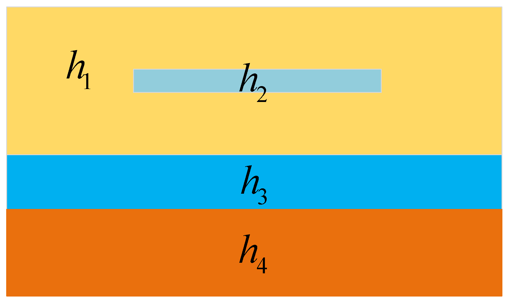
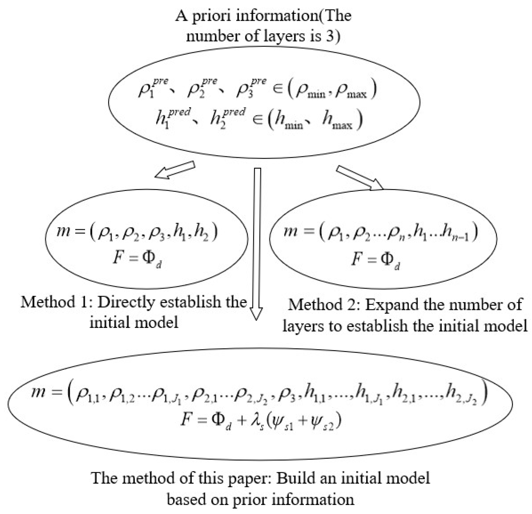
2. Piecewise Regularized Inversion Method

Nonlinear inversion involves an iterative search for the optimal solution based on a strict transient electromagnetic forward formula, objective function, and initial model, following the search principle of the algorithm and the objective function [23]. The regularized objective function for transient electromagnetic data inversion includes fitting and roughness constraint functions for models. The expression is as follows:

$$F={\varphi }_d+\lambda {\psi }_m$$

(1)

where ${\varphi }_d$ represents the data fitting functional, ${\psi }_m$ represents the roughness constraint function, and $\lambda$ denotes the regularization factor.

The appropriate data function is constructed using the L1 norm, which has both advantages and disadvantages compared to the L2 norm. While the L2 norm offers smooth and continuous characteristics, the L1 norm is more tolerant of extreme fitting errors and is more effective in describing layered boundaries [24]. The formula is as follows:

$${\varphi }_d={\displaystyle \sum _{i=1}^N\left|\left(D_i^{obs}-G_i(m)\right)/D_i^{obs}\right|}/N$$

(2)

the model constraint function imposes constraints on the conductivity change rate of each layer in the vertical direction, expressed as follows:

$${\psi }_m={\displaystyle \sum _{i=1}^{N-1}{(m_{i+1}-m_i)}^2}/h_i\left(N-1\right)$$

(3)

where $D^{obs}$ is the observation data vector; $N$, $m$, $h$ represent the number of layers, resistivity parameters, and layer thickness parameters of the prediction model, respectively; and $G$ is the forward operator.

The initial model is established based on prior information, including model parameters such as the resistivity and thickness of each layer. The initial model is constructed using available a priori information, which is typically obtained from conductivity-depth imaging methods or borehole data. For instance, consider a low-resistivity anomaly with a small thickness in a specific geological structure, as shown in Figure 1. Figure 2 illustrates different methods for constructing the initial model. Method 1 involves the direct establishment of the initial model; however, when information about thin layers with low resistivity is not readily available from prior information, the model must use the parameters of three layers to fit the geological structure of five layers, resulting in poor fitting performance. Method 2 assigns a relatively large number of layers in the initial model, which mitigates the impact of parameter uncertainty on the inversion results to some extent; however, increasing the number of layers exacerbates the non-uniqueness of the inversion and makes it challenging to discern the model results, posing new challenges.

To address the issues with existing methods, this paper proposes a new method for designing the initial model, consisting of two main parts. First, based on the initial model established using Method 1, each layer except the bottom layer is further subdivided, and the model parameters are expressed as follows:

$$m_i=[{\rho }_{i,1},{\rho }_{i,2},...{\rho }_{i,J_i}],h_i=[{\delta }_{i,1},{\delta }_{i,2},...{\delta }_{i,J_i}],0<i<N$$

$$h_{i,\min }\le ({\delta }_{i,1}+{\delta }_{i,2}+...+{\delta }_{i,\mathrm{Ji}})\le h_{i,\max }$$

$$m_{i,\min }\le ({\rho }_{\mathrm{i},1},{\rho }_{\mathrm{i},2},...,{\rho }_{\mathrm{i},\mathrm{Ji}})\le m_{i,\max }$$

(4)

where $N$ denotes the number of segments divided according to the a priori information; $[h_{i,\mathrm{m}\mathrm{i}\mathrm{n}},h_{i,\mathrm{m}\mathrm{a}\mathrm{x}}]$ and $[m_{i,\mathrm{m}\mathrm{i}\mathrm{n}},m_{i,\mathrm{m}\mathrm{a}\mathrm{x}}]$ are the upper and lower bounds of the layer thickness and resistivity in the $i$-th segment, respectively; and $J_i$ is the number of inner layers divided in each segment. $\left[{\rho }_{i,1},{\rho }_{i,2},\dots ,{\rho }_{i,J_i}\right]$ and $\left[{\delta }_{i,1},{\delta }_{i,2},\dots ,{\delta }_{i,J_i}\right]$, respectively, represent the resistivity parameters and layer thickness parameters after subdividing $m$ into $J_i$ layers. In the case where $[h_{i,\mathrm{m}\mathrm{i}\mathrm{n}},h_{i,\mathrm{m}\mathrm{a}\mathrm{x}}]$ is known, it is only necessary to select the inner layer thickness range, i.e., $[{\delta }_{i,\mathrm{m}\mathrm{i}\mathrm{n}},{\delta }_{i,\mathrm{m}\mathrm{a}\mathrm{x}}]$, to obtain the number of inner layers, J_i, in the i-th segment.

As depicted in Figure 3, for the selection of $[{\delta }_{i,\mathrm{m}\mathrm{i}\mathrm{n}},{\delta }_{i,\mathrm{m}\mathrm{a}\mathrm{x}}]$, it primarily depends on two factors: one is selecting appropriate upper and lower boundary values based on the required layering accuracy in actual exploration, and the other considers the fact that the inversion accuracy of transient electromagnetic data gradually decreases with increasing depth. Hence, the threshold value for the change in layer thickness is set to increase with depth (e.g., during synthetic data simulation, it is set as within 200 M, more than 200 M, and more than 400 M of predicted depth, and the layer thickness thresholds are set to [5, 25], [10, 50], and [20, 100], respectively). Second, since transient electromagnetic inversion exhibits highly nonlinear characteristics, introducing a regularization constraint for model smoothing is crucial to reduce false anomalies and enhance the model fitting effect. Therefore, segmental regularization constraints are incorporated to construct the objective function, expressed as follows:

$$F={\varphi }_d+{\displaystyle \sum _{i=1}^{N-1}({\lambda }_i{\psi }_i)}$$

(5)

where ${\psi }_i$ is the vertical model constraint inside the model in the segment, and ${\lambda }_i$ is the regularization weight of the segment model.

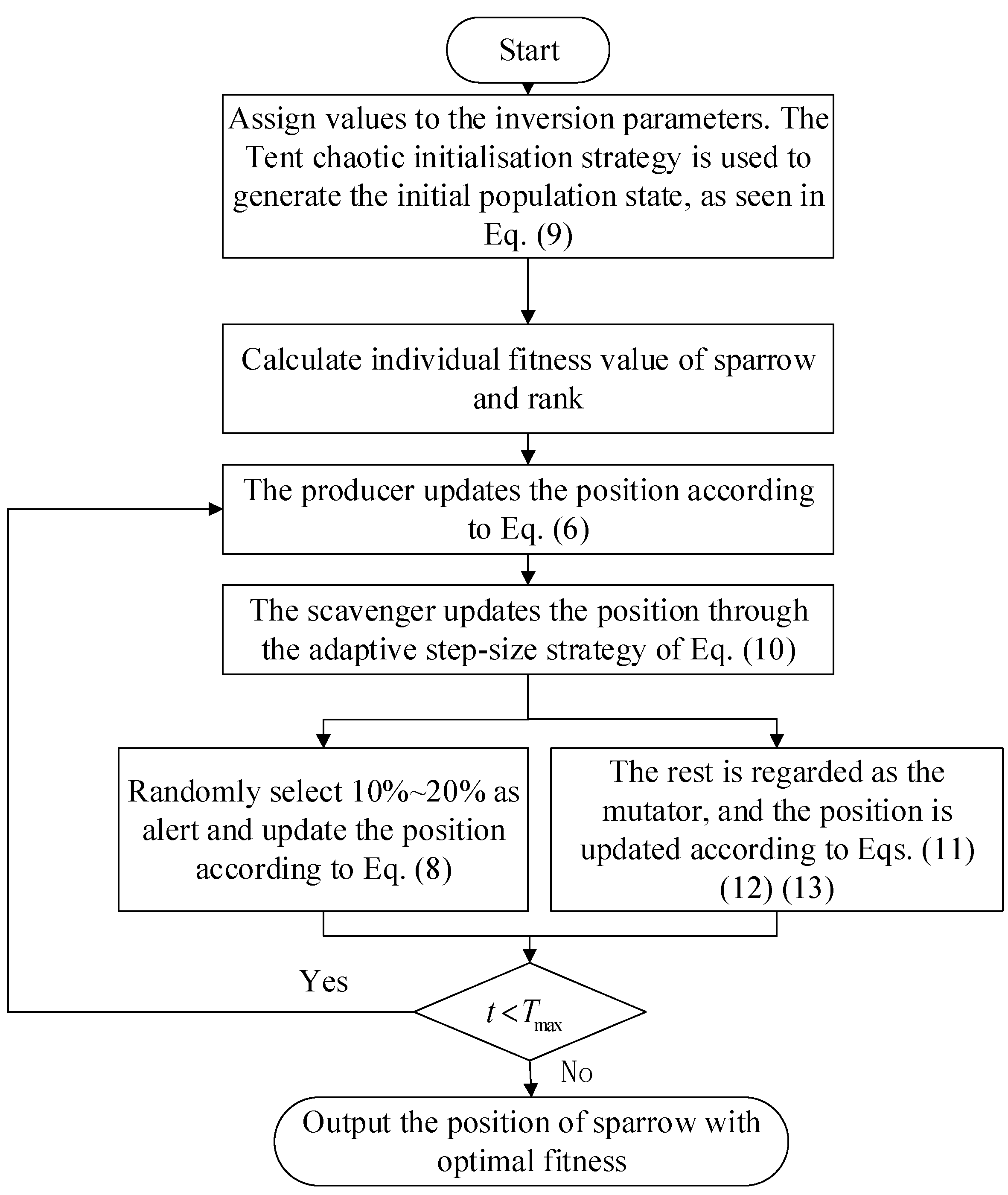
3. Improved Sparrow Search Algorithm

3.1. Sparrow Search Algorithm

The SSA primarily simulates the foraging behavior of sparrows, employing a producer–scrounger model with a detection and early warning mechanism. The SSA simulated the process of individual sparrows avoiding natural enemies and getting closer to food. The population consists of three roles: producer, scrounger, and alert. Producers have a high energy reserve and a larger foraging area, which can provide foraging area and direction information for the population. Scroungers approach producers and grab food resources. The alert can give a warning signal when danger is coming, and if necessary, give up food to avoid danger.

• Step 1: The producer location update

Among the sparrow population, producers with good adaptability have priority access to food during foraging. They provide search directions for all scroungers. Typically, producers make up around 10% to 20% of the population. The sparrow population is represented by a matrix $X$ with n rows and d columns. $n$ is the population quantity. $d$ represents the number of parameters for sparrows. The location update formula is as follows:

$$X_{i,j}^{t+1}=\left\{\begin{array}{c}{X}_{i,j}^t\cdot \exp \left(-i/\left(\alpha \cdot T_{\max }\right)\right),R<ST\\ X_{i,j}^t+Q\cdot U,R\ge ST\end{array}\right.,R\in [0,1],ST\in [0.5,1]$$

(6)

where $X_{i,j}^{t+1}$ represents the position information of the $j$-th dimension of the $i$-th sparrow at the t + 1st iteration. $T_{max}$ is the maximum number of iterations, $\alpha$ is a uniform random number between (0, 1], $U$ is $d\times 1$ Matrix with elements of 1, $Q$ is an $d$-dimensional row vector with elements that are random numbers following a normal distribution, and $R$ and $ST$ represent the alarm value and the safety threshold, respectively. When $R<ST$, this indicates that the foraging environment is safe and that producers can conduct an extensive search. Otherwise, it indicates the presence of a predator threat, and producers adjust their search strategy to conduct a smaller search around themselves.

• Step 2: Scroungers position update

Apart from producers, the remaining sparrows are scroungers. The location update formula is as follows:

$$X_{i,j}^{t+1}=\left\{\begin{array}{c}{Q}_j\cdot \exp \left(X_{worst,j}^t/t\right),i>\frac{n}{2}\\ X_{p,j}^{t+1}+\left|X_i^t-X_p^{t+1}\right|A^{+},i\le \frac{n}{2}\end{array}\right.$$

(7)

where $X_{worst}$ represents the worst of sparrows in the current population, $X_p$ is the optimal position occupied by producers, $n$ is the population quantity, $A$ represents a matrix of $1\times d$ for which each element inside is randomly assigned 1 or −1, and $A^{+}=A^T{\left(A{A}^T\right)}^{-1}$. When $i>0.5n$, scroungers are less adaptable and must immediately fly away from their current area to forage in different areas. Conversely, scroungers are moderately adaptable and move closer to the current optimal position to search for food.

• Step 3: Alert position update

To ensure safe foraging, 10% to 20% of sparrows are randomly selected as alerts in each round. The location update is as follows.

$$X_{i,j}^{t+1}=\left\{\begin{array}{c}{X}_{best,j}^t+\beta \left(X_{i,j}^t-X_{best,j}^t\right),f_i>f_{best}\\ X_{i,j}^t+K\left(X_{i,j}^t-X_{worst,j}^t\right)/\left|f_i-f_{worst}\right|,f_i\le f_{best}\end{array}\right.$$

(8)

In this formula, β and K are random numbers within the range [0, 1], and f is the fitness value of the sparrow. When $f_i>f_{best}$, it indicates that an alert is located at the edge of the population and thus moves closer to the center of the population distribution. Conversely, if $f_i\le f_{best}$, an alert is positioned within the population and moves away from the edge of the sparrow population due to the awareness of a predator threat.

3.2. Tent Chaotic Mapping

The initial populations in the SSA are typically generated at random locations, which may not ensure sufficient diversity in the pre-population. Utilizing the chaotic properties of Tent mapping results in better traversal uniformity and sensitivity to initial values. This, in turn, leads to the faster convergence of the algorithm [25]. The expression for the initial population sequence $X$ in the SSA, after invoking Tent chaotic mapping, is as follows:

$$Z_i^{j+1}=\left\{\begin{array}{c}{Z}_i^j/r,0\le Z_i^j\le r\\ \left(1-Z_i^j\right)/\left(1-r\right),r<Z_i^j\le 1\end{array}\right.$$

$$X_{i,j}=X_{i,j(\min )}+Z_i^j\left(X_{i,j(\max )}-X_{i,j(\min )}\right)$$

(9)

where $i$ represents different sparrow individuals, $j$ $(j\le d)$ in $Z_i^j$ represents both the number of iterations and the change in dimension, and $r$ is a random number between 0 and 1 to maintain the randomness of the algorithm’s initialization information. Further, the initial position sequence of individual sparrow positions within the search area, $X_{i,j\left(max\right)}$ and $X_{i,j\left(min\right)}$, represent the lower and upper limits of $X_{i,j}$, respectively.

3.3. Adaptive Step-Size Adjustment Strategy for Scrounger Position Update

From the scrounger update formula, it is evident that the joiner will approach the scroungers’ optimal position with a certain probability, but individual consideration of the scroungers’ step size to move closer to the producers’ optimal position is lacking. In general, individuals already near the optimal position should take smaller steps to prevent premature clustering, while those far from the optimal position should move closer more rapidly due to poor adaptation. To address this, we introduce an adaptive step factor to control the distance between the scroungers and the producers’ dimensions. When the scroungers and scroungers’ optimal positions are farther apart, the step size increases to enhance algorithm convergence speed, and conversely, reducing the step size slows down clustering speed and improves the local search capability. Their position is updated as follows:

$$X_i^{t+1}=\left\{\begin{array}{c}Q\cdot \exp \left(X_{worst}^t/t\right),i>\frac{n}{2}\\ X_{best}^{t+1}+D_{i,j}\cdot \left|X_i^t-X_{best}^t\right|A^{+},i\le \frac{n}{2}\end{array}\right.$$

$$D_{i,j}=s+\left(1-s\right)\cdot \left|X_i^t-X_{best}^t\right|/S_j$$

(10)

where $i$ denotes different scrounger individuals sorted by fitness, $j$ denotes dimension, and $D_{i,j}$ represents the adaptive step factor. $s$ is taken from 0.01 to 0.2, and $S$ is the maximum value of the distance between the scrounger and the optimal producer in the $j$-th dimension for the current number of iterations.

3.4. Differential Variational Operators

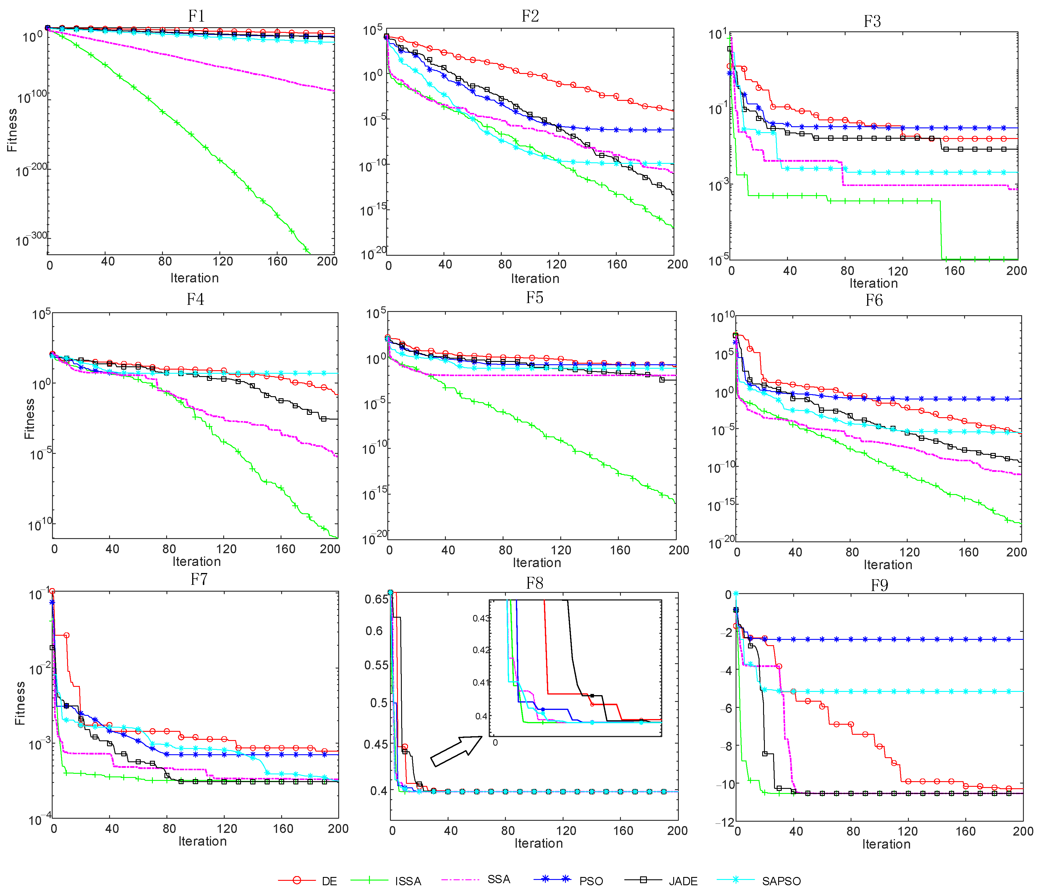
In the original sparrow search algorithm, position updates primarily rely on the information of individuals with the best or worst fitness values with limited use of other individuals’ location information, which may not facilitate the search for a globally optimal solution to the objective function. To address this, the differential variation operator is introduced to update individual positions other than the alerts, utilizing all ignored individual information and enhancing the algorithm’s global exploration ability. The differential variation operator comprises the following main steps.

Firstly, mutation operations create new individuals, and the update formula is as follows:

$$v_i=X_{r1}+F0\cdot \left(X_{r2}-X_{r3}\right)$$

(11)

$F0$ is the variance factor; $r1$, $r2$, and $r3$ denote sequences of mutually unequal random individuals within the population; and $v_i$ represents the $i$-th individual of the mutated sparrow population.

The cross-factor is $CR$. $X_{i,j}$ and $v_{i,j}$ denote the location information of the $i$-th sparrow in the $j$-th dimension, respectively. The variance vector ($v_{i,j}$) is crossed with the parent base vector ($X_{i,j}$) following the crossover probability to obtain a new offspring individual. The crossover formula is as follows:

$$u_{i,j}=\left\{\begin{array}{c}{v}_{i,j},rand<CR\cup j=j_{rand}\\ X_{i,j},rand>CR\cap j\ne j_{rand}\end{array}\right.$$

(12)

According to the greedy principle, the appropriate individual is selected from the offspring population to be the parent population of the next generation.

$$X_i^{t+1}=\left\{\begin{array}{c}{u}_i^t,fit(u_i^t)<fit(X_i^t)\\ X_i^t,fit(u_i^t)\ge fit(X_i^t)\end{array}\right.$$

(13)

Figure 4 illustrates the fundamental process of enhancing the sparrow search algorithm.

4. Function Test

To validate the feasibility and optimization ability of the ISSA, we selected nine benchmark functions for comparison and tested them against the SSA, PSO, SAPSO (self-adaptive particle swarm optimization), DE, and JADE (adaptive differential evolution with optional external archive). In the tests, the population size was set to 100, and the maximum number of iterations was 200. Finally,

Table 1. Comparison of test function results.

Serial Number	Function	Dimension	Range	Theoretical Value	ISSA	SSA	DE	JADE	PSO	SAPSO
F1	Sphere	30	[−100, 100]	0	0 × 100	4.5 × 10−87	4.8 × 10−5	1.8 × 10−10	8.4 × 10−9	1.3 × 10−17
F2	Step	10	[−100, 100]	0	1.3 × 10−17	8.5 × 10−12	7.7 × 10−9	4.7 × 10−14	6.1 × 10−7	1.3 × 10−10
F3	Quartic	10	[−1.28, 1.28]	0	1.1 × 10−5	6.3 × 10−4	1.6 × 10−2	8.2 × 10−3	3 × 10−2	2 × 10−3
F4	Generalized Rastrigin’s	10	[−5.12, 5.12]	0	1.3 × 10−10	3.1 × 10−6	1.5 × 10−1	3 × 10−3	9.9 × 100	5 × 10−0
F5	Griewank’s	10	[−600, 600]	0	1 × 10−16	7 × 10−3	9 × 10−2	3 × 10−3	1.5 × 10−1	6 × 10−2
F6	Generalized Penalized	10	[−50, 50]	0	2.5 × 10−18	1.4 × 10−11	2.1 × 10−6	3.5 × 10−10	9 × 10−3	3.2 × 10−6
F7	Kowalik’s	4	[−5, 5]	3 × 10−4	3 × 10−4	3.3 × 10−4	8 × 10−4	3 × 10−4	7.1 × 10−4	3.3 × 10−4
F8	Branin	[a, b]	$\mathrm{a} \in$ [−5, 10], $\mathrm{b} \in$ [0, 15]	3.9 × 10−1	3.9 × 10−1	3.9 × 10−1	3.9 × 10−1	3.9 × 10−1	3.9 × 10−1	3.9 × 10−1
F9	Shekel’s Family	4	[0, 10]	−10	−10	−5.1	−10	−10	−2.4	−5.2

summarizes the results.

The above comparative experiments analyze the proposed algorithm’s superiority from unimodal, multimodal, high-dimensional, and low-dimensional perspectives. The ISSA achieved the theoretical optimal value of 0 only when solving F1 among the three unimodal high-dimensional functions, F1, F2, and F3; however, for F2 and F3, the optimization performance difference between the ISSA, SSA, and JADE is relatively small, with the ISSA being the closest to the theoretical optimal. Among the three high-dimensional multimodal functions, F4–F6, the ISSA demonstrated a significant advantage in optimization performance. For the three low-dimensional multimodal functions, F7–F9, both the ISSA and JADE identified the theoretical optimal values. In contrast, the unimproved SSA and DE failed to find the theoretical optimal solutions in F9 and F7, respectively.

To compare the algorithm’s convergence speed, a convergence curve graph is provided for the above experiment, as shown in Figure 5. It is evident from the graph that ISSA’s convergence speed is superior to other algorithms in most cases, particularly for high-dimensional function optimization. The ISSA is more likely to escape local optimal solutions than the SSA. Additionally, for optimizing low-dimensional multimodal functions (F7–F9), while the optimization accuracy of the ISSA is not significantly different from that of JADE, the SSA, DE, and the ISSA still exhibits speed advantages. Based on the above analysis, it can be concluded that ISSA offers improved optimization performance and stability.

5. Inversion Test of an Ideal Model

The ISSA algorithm was employed to perform inversion tests on theoretical data from a long-wire transient electromagnetic source to investigate the influence of different regularization factors and initial models on the fit of the final model. The forward response of the long-wire source was derived using a linear digital filtering algorithm with the following measurement setup parameters: a transmission cable length of 1000 M, a transmission current of 10 A, a receiver coil area of 1 M², a source–receiver horizontal offset distance of 100 M, and an observation time interval with logarithmic spacing between 0.001 and 20 ms.

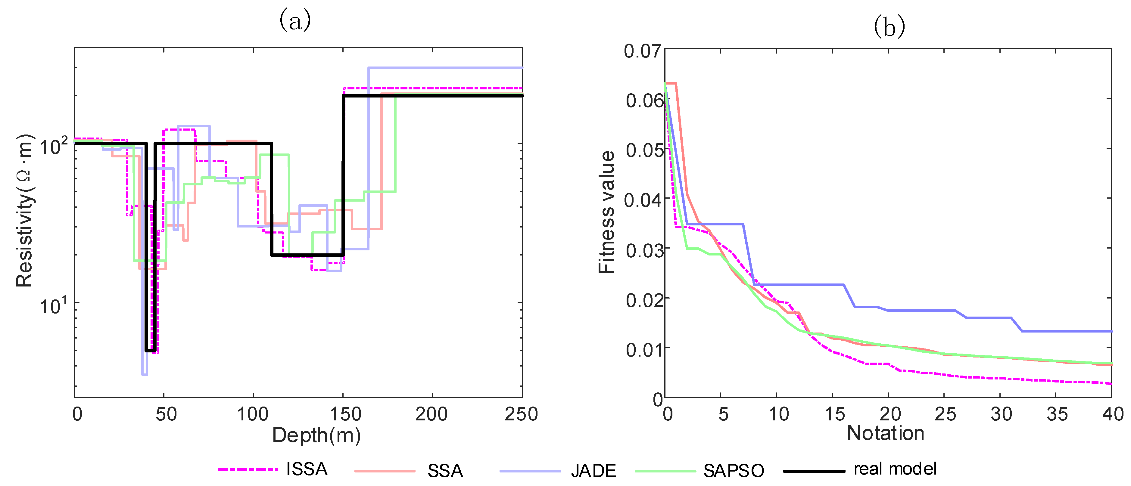
5.1. Inversion Performance Analysis of the Algorithm

In this section, the performance of each algorithm when applying a 1D TEM inversion is explored. For this purpose, a five-layer layered model was built and inverted using four algorithms in the following order: the ISSA, SSA, JADE, and SAPSO. The control parameters of the algorithms are detailed in

Table 2. Control parameter settings for ISSA.

Notation	Clarification	Value
n	Population size	100
M	Maximum number of iterations of the algorithm	50
ST	Safety threshold	0.8
P	Discoverers as a proportion of population size	0.2
F0	Variance factor	0.4
CR	Cross-factor	0.2

, and the number of layers of the inversion model was set to 15.

As the number of inversion model layers is not the same as the number of real model layers, we adopted the discretized mean square error of model fitting (D-MSE) as the evaluation criterion for the inversion results. The D-MSE is calculated as follows:

$$MS{E}_D={\displaystyle \sum _{i=1}^K\left|{\log }_{10}\left({\rho }_{Ti}/{\rho }_{Ci}\right)\right|}/K$$

(14)

where $K$ is the total number of discrete values between the surface and the maximum depth boundary (here, we take $K=300$), ${\rho }_T$ is the theoretical resistivity at each depth after the discretization of the test model, and ${\rho }_C$ is the calculated value of resistivity after discretisation of the inverse model.

Figure 6 shows the results obtained by taking the median of the values of D-MSE after 11 experimental inversions. At first, in the inverse model comparison graph, although the effects of various algorithms show the changing trend of the real model, it is evident that the curve change of the ISSA closely resembles the real model. For the fitness curve, the convergence speed of the ISSA in the early stage is similar to that of the SSA and SAPSO. Still, going out of the local optimal solution is more accessible because more population diversity is retained in the optimization process. In order to verify the robustness of the algorithm, 5% and 10% Gaussian random noise (the orthogonal response data multiplied by a percentage) was added to the TEM synthetic data, and the results are shown in

Table 3. Comparison of averages of model evaluation parameters for 11 inversion results.

Algorithm	Without Noise		5% Noise		10% Noise
	Fitness Value	D-MSE	Fitness Value	D-MSE	Fitness Value	D-MSE
ISSA	0.0031	0.1182	0.0065	0.1298	0.0123	0.1893
SSA	0.0065	0.1966	0.0095	0.2255	0.0165	0.2563
JADE	0.0103	0.2299	0.01424	0.2177	0.0224	0.2388
SAPSO	0.0059	0.1945	0.0086	0.2013	0.0157	0.2255

. The final results of the ISSA are significantly better than the other algorithms at both no noise and 5% noise, and 5% noise has a lesser effect on the model fitting results. In contrast, after the addition of 10% Gaussian random noise, the ISSA’s model fitting decreases, but its accuracy is still higher.

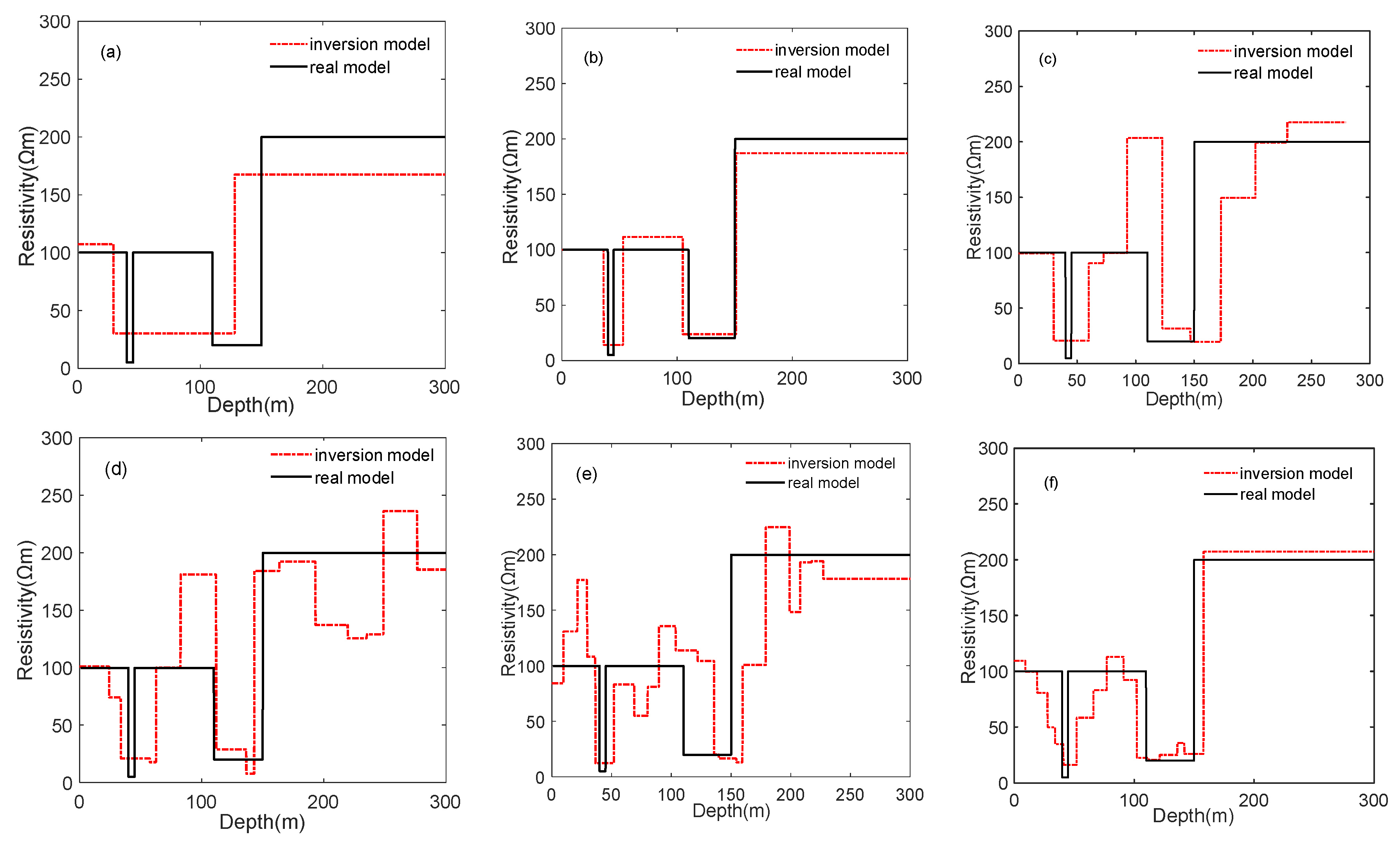
5.2. One-Dimensional Three-Layer Model Test

Inversion tests were conducted on the regularization factors (${\lambda }_1~{\lambda }_7$) using a three-layer H-type resistivity model to select the regularization weight corresponding to the threshold value of each layer thickness. The inversion was performed using a segmented regularization model, where the layer-like low-resistance distribution of the three H-type models was located at depths of 70~80 M, 250~300 M, and 500~600 M with corresponding inner layer thickness thresholds of, respectively, J₁ (2~25 M), J₂ (5~50 M), and J₃ (10~100 M). Additionally, to verify the stability of the regularization factors under different resistivity ratios of the intermediate layer and the background layer (${\sigma }_r$), tests were conducted using ${\sigma }_r=5$ and ${\sigma }_r=40$. In the three-layer H-type model,

$${\sigma }_r=\left({\rho }_1+{\rho }_3\right)/\left(2{\rho }_2\right)$$

(15)

where $\rho$ represents the resistivity of each layer.

Considering the probability distribution properties of the algorithm, we selected the results corresponding to the median of D-MSE in 11 inversions. The results are presented in

Table 4. Mean square error of inversion curve of three-layer H-type model under different layer thickness thresholds, regularization factors, and resistivity ratios.

Layer Thickness Threshold	Resistivity Ratio	D-MSE
		${\mathit{\lambda }}_1$ $(2\times {10}^{-3})$	${\mathit{\lambda }}_2$ $(6\times {10}^{-4})$	${\mathit{\lambda }}_3$ $(2\times {10}^{-4})$	${\mathit{\lambda }}_4$ $(6\times {10}^{-5})$	${\mathit{\lambda }}_5$ $(2\times {10}^{-5})$	${\mathit{\lambda }}_6$ $(6\times {10}^{-6})$	${\mathit{\lambda }}_7$ $(2\times {10}^{-6})$
J1	${\sigma }_r=5$	0.1930	0.0833	0.0553	0.1052	0.1642	0.1264	0.4442
	${\sigma }_r=40$	0.2471	0.3109	0.2045	0.1874	0.1219	0.1096	0.2647
J2	${\sigma }_r=5$	0.2020	0.0704	0.1149	0.1442	0.2062	0.2385	0.6767
	${\sigma }_r=40$	0.2784	0.1601	0.1952	0.1683	0.0673	0.1547	0.1881
J3	${\sigma }_r=5$	0.2078	0.0937	0.0833	0.1079	0.1310	0.2041	0.3827
	${\sigma }_r=40$	0.2543	0.2178	0.1727	0.1614	0.1325	0.1863	0.2603

. The data comparison in Table 4 reveals that the regularization factor (${\lambda }_{min}$) associated with the minimum MF-MSE for each row is approximately located around ${\lambda }_3$ and ${\lambda }_5$ when ${\sigma }_r$ is 5 and 40, respectively. This indicates that the size of ${\sigma }_r$ significantly influences the selection of the regularization factor under the specified threshold of layer thickness. The inversion results for ${\lambda }_1$, ${\lambda }_7$, and ${\lambda }_{min}$ are depicted in Figure 7 and Figure 8.

From the figures, it is evident that the curve of ${\lambda }_7$ exhibits poor smoothness in resistivity at multiple points. This suggests that the non-uniqueness of the inversion is exacerbated, and the results may be inadequate when the regularization constraint is too weak. Conversely, the curve of ${\lambda }_1$ corresponds to a situation where the regularization constraint is overly strong. In Figure 7, where ${\sigma }_r=5$, not only is there a significant shift in the boundary of the target body but also the overall inversion performance needs improvement. In Figure 8, as ${\sigma }_r$ increases, the fitting of the inversion to low resistivity improves to some extent, but the curve of the inversion result becomes excessively smooth, leading to reduced accuracy. The curve of ${\lambda }_{min}$ strikes a relative balance and does not exhibit significant false anomalies. The inversion results accurately reflect the low resistivity characteristics of the H-type model at the corresponding depth and are generally consistent with the actual model’s resistivity distribution.

5.3. One-Dimensional Five-Layer Model Test

After establishing the layering principle and regularized weights, a geoelectric model in the shape of HKH with five HKH-type layers was created. This model was used to compare the effects of nonlinear inversion using various methods for the initial model design. The parameter settings are as follows: the resistivity of the first to fifth layers is, in order, 100, 5, 100, 20, and 200 ΩM, and the layer thickness of the first to fourth layers is 40, 5, 65, and 40 M.

To assess the influence of different initial model design methods for nonlinear inversion, the initial model sets the range of inversion model parameters for the first three layers only, where $m_1$ is 2~200 ΩM, $m_2$ is 3~100 ΩM, $m_3$ is 5~400 ΩM, $h_1$ is 40~200 M, and $h_2$ is 20~100 M. Figure 9 presents a comparison of the inversion results using the segmented regularization method with different numbers of initialized layers.

It can be observed that due to the parameter uncertainty of the prior information, directly designing the initial model leads to too few model parameters and low fitting degrees, as shown in Figure 9a. The inversion result is relatively good when the initial model parameters correspond to the actual model parameters, as shown in Figure 9b; however, determining the required initial model parameters when inverting massive actual data is often challenging.

When considering the use of more layers to avoid the problem of having too few parameters, it partially mitigates the influence of parameter uncertainty; however, due to the excessive number of layers, false anomalies appear to varying degrees, as shown in Figure 9c,d,f, and the robustness and clarity of the inversion model suffer.

The proposed method of segmental regularization adopts the J₁-type layer thickness threshold and the regularization factor of ${\lambda }_3$ (2 × 10⁻⁴). The inversion results are presented in Figure 9e and accurately identify the low-resistivity anomaly near a depth of 50 M and demonstrate excellent performance in delineating the high–low resistivity boundaries near depths of 100 M and 150 M. The establishment of regularization constraints in the inner layers significantly improves the smoothness of the model. Moreover, the requirement for prior information in the design of the initial model is relatively low, making it more practical and tolerant of errors. In comparison to the other initialization methods described earlier, this method can more reliably obtain a straightforward electrical interface.

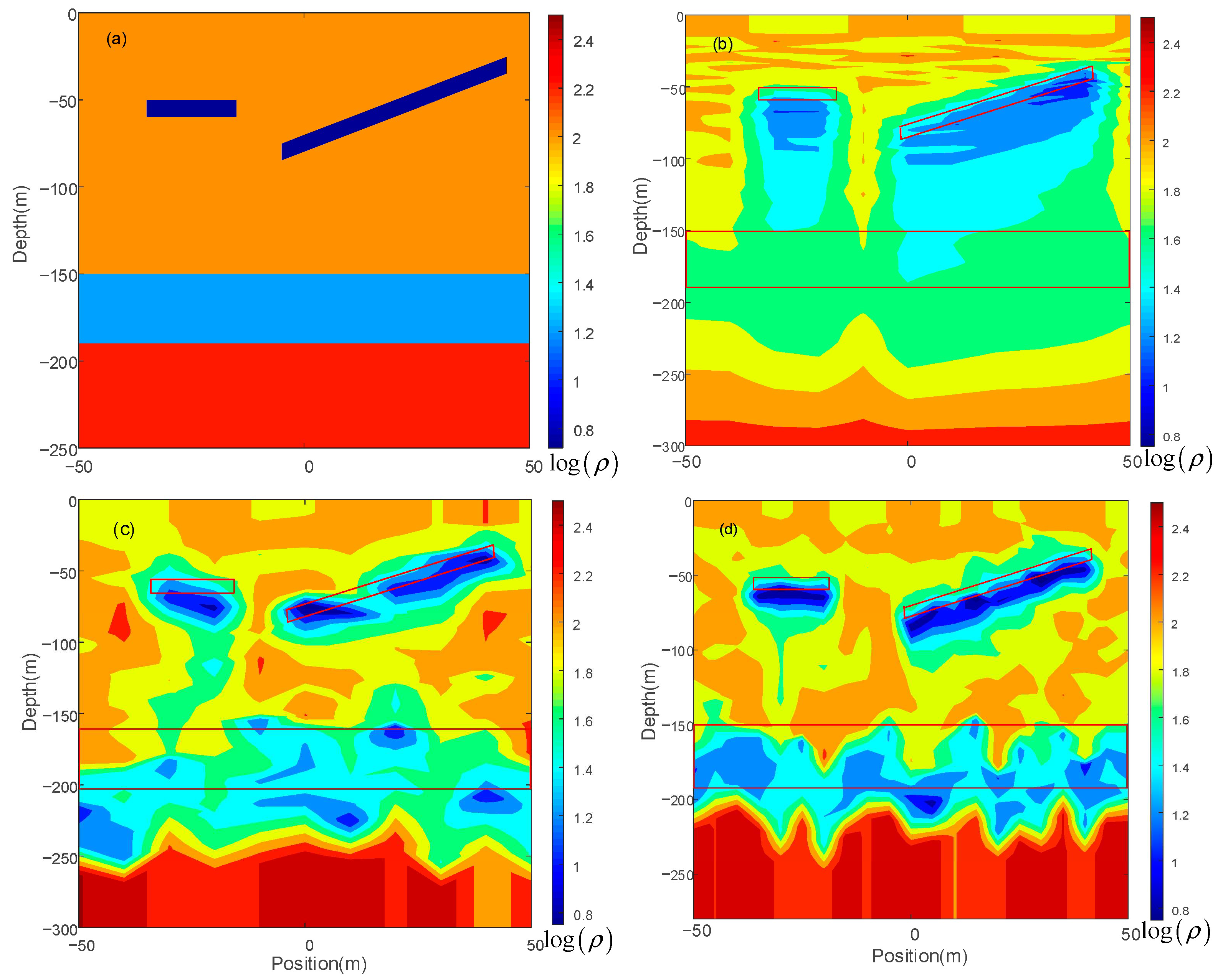
5.4. Two-Dimensional Model Inversion Test

To assess the effectiveness of the ISSA inversion method in comparison to other algorithms, a theoretical model with an electrical structure was designed, as depicted in Figure 10a. The model background consists of a three-layer H-shaped geoelectric structure and includes two low-resistivity thin plate anomalies, one in the horizontal direction and the other at an oblique angle. There are 11 measurement points spaced at intervals of 10 M along the conductor source. The data obtained from the 1D inversion of these 11 measurement points using various algorithms were interpolated and smoothed to generate the cross-sectional images shown in Figure 10b–d.

Figure 10b presents the results obtained using the traditional OCCAM smooth inversion method. In this image, the resolution for depicting low-resistivity layers at depths of 150–190 M is inadequate. Additionally, the accurate resistivity information between the shallow low-resistivity thin plate and the underlying low-resistivity layer is obscured. This method is not suitable for geological regions with continuous resistivity changes.

In contrast, the results obtained through nonlinear methods, as shown in Figure 10c,d, effectively overcome the issue of low accuracy and exhibit greater sensitivity to changes in the resistivity of geological layers with fewer boundary ambiguities; however, the stability of the inversion using the original SSA algorithm is insufficient, as shown in Figure 10c. The inversion result for the low-resistivity thin layer deviates from the theoretical model. In comparison, the result obtained using the ISSA algorithm, as shown in Figure 10d, is closer to the actual geological structure as a result of more explicit boundaries and more precise anomaly location determination.

6. Field Data Inversion

This study utilized field profile data obtained from a mining area in Chongqing city to validate the inversion performance. The experiment was conducted along a measurement line stretching 310 M with a point spacing of 10 M. A Terra TEM transient electromagnetic system manufactured in Australia was employed for this purpose. The transmitter current used was approximately 12 A, and the receiving coil was a small loop with a side length of 2.5 M and contained 20 turns.

Five inversion attempts were carried out using various algorithms, and the average results were recorded. Figure 11 compares the attenuation voltage measured by the receiving coil at a distance of 0 m on the measurement line with the forward response obtained using different algorithms. The field data exhibited fluctuations due to external noise interference. In comparison to other algorithms, the inversion data from the ISSA are generally consistent with the field data and exhibit a higher degree of fitting. The average fitness values for the ISSA, SSA, JADE, and SAPSO are 0.0043, 0.0171, 0.0398, and 0.0394, respectively, serving as a criterion for assessing the algorithm’s feasibility. By combining existing geological data and drilling records, we infer that the depth of 0–30 M consists of mudstone with a slightly higher resistivity. The low-resistivity anomaly body observed around 30–80 M corresponds to a strip distribution consistent with the spatial layout of the goaf and is inferred to be the coal mining goaf water accumulation zone. The region below 120 M comprises relatively intact and dense rock ore with minuscule pores, low groundwater content, and relatively high resistivity.

Figure 12 displays the inversion results obtained using four algorithms: SAPSO, JADE, SSA, and ISSA. Upon comparison, it becomes evident that the inversion result achieved through the ISSA algorithm (Figure 12c) better reflects the geological characteristics of the Empty Ponding District. This indicates that the segmented regularization method based on the ISSA, as proposed in this study, is suitable for processing field data. The inversion results effectively portray underground anomalous geological bodies.

7. Conclusions

This article introduces a segmented regularization inversion method designed for transient electromagnetic data. The approach involves creating a segmented initial model based on preliminary information, taking into account the predicted depths and thickness thresholds for each layer. It applies segmented regularization principles to constrain the objective inversion function. One-dimensional numerical simulation examples highlight that the segmented initial model exhibits greater fault tolerance compared to the commonly used direct initial model scheme. This feature reduces the impact of parameter uncertainty when dealing with complex geological structures, rendering it more widely applicable.

Furthermore, the article incorporates the newer sparrow search algorithm (SSA) into nonlinear algorithms and employs it for the two-dimensional theoretical model inversion of transient electromagnetic data. The results indicate that the SSA outperforms the traditional OCCAM linear method in terms of recovering the electrical model. The SSA exhibits global search capabilities and quick convergence but tends to approach local optima in the later stages of evolution. Additionally, the inversion results at each measurement point are less stable. The enhanced ISSA, based on the SSA, delivers inversion results that closely align with the original electrical model. It boasts several advantages, including reduced error fluctuations, improved noise resistance, enhanced inversion accuracy, and greater stability. This suggests that the improved algorithm is more effective in addressing geophysical inversion challenges.

Nonetheless, due to the inherent randomness of model updates in nonlinear inversion algorithms, using segmented initial models can lead to increased complexity as the number of model layers grows. This results in a slower optimization speed and longer convergence times. Although regularization constraints have somewhat enhanced the inversion efficiency, the time cost associated with differences in optimization speed between a two-dimensional and three-dimensional inversion remains substantial; therefore, improving the optimization efficiency of a nonlinear inversion in higher dimensions remains an ongoing area of research.

References

1. McNeill, J.D. Application of Transient Electromagnetic Techniques; Geonics Limited: Missasauga, ON, Canada, 1980; 17p. [Google Scholar]
2. Yang, D.; Oldenburg, D.W. Three-dimensional inversion of airborne time-domain electromagnetic data with applications to a porphyry deposit. Geophysics 2012, 77, B23–B34. [Google Scholar] [CrossRef]
3. Qian, W.; Xu, Y.; Gu, Z.; Xiang, Z.; Li, Z.; Liu, J.; Wu, J. Characterisation of transient electromagnetic signals during fixed interference sources in tunnel structure. Math. Biosci. Eng. 2021, 18, 6907–6925. [Google Scholar] [CrossRef]
4. Ezersky, M.; Legchenko, A.; Al-Zoubi, A.; Levi, E.; Akkawi, E.; Chalikakis, K. TEM study of the geoelectrical structure and groundwater salinity of the nahal hever sinkhole site, dead sea shore, Israel. J. Appl. Geophys. 2011, 75, 99–112. [Google Scholar] [CrossRef]
5. Su, B.; Yu, J.; Sheng, C.; Zhang, Y. Maxwell-equations based on mining transient electromagnetic method for coal mine-disaster water detection. Elektron. Ir. Elektrotechnika 2017, 23, 20–23. [Google Scholar] [CrossRef]
6. Li, Z.; Huang, Q.; Xie, X.; Tang, X.; Chang, L. A Generic 1D Forward Modeling and Inversion Algorithm for TEM Sounding with an Arbitrary Horizontal Loop. Pure Appl. Geophys. 2016, 173, 2869–2883. [Google Scholar] [CrossRef]
7. Haroon, A.; Adrian, J.; Bergers, R.; Gurk, M.; Tezkan, B.; Mammadov, A.L.; Novruzov, A.G. Joint inversion of long-offset and central-loop transient Electromagnetic Data: Application to a mud volcano exploration in Perekishkul, Azerbaijan. Geophys. Prospect. 2015, 63, 478–494. [Google Scholar] [CrossRef]
8. Yang, H.-Y.; Li, F.-P.; Chen, S.-E.; Yue, J.-H.; Guo, F.-S.; Chen, X.; Zhang, H. An inversion of transient electromagnetic data from a conical source. Appl. Geophys. 2018, 15, 545–555. [Google Scholar] [CrossRef]
9. Wang, S.; Di, Q.; Xia, T.; Ren, Z.; Song, J.; Zou, G. Transient electromagnetic method inversion based on Lévy flight-particle swarm optimization. Chin. J. Geophys. 2022, 65, 1482–1493. (In Chinese) [Google Scholar] [CrossRef]
10. Li, R.; Yu, N.; Li, R.; Zhuang, Q.; Zhang, H. Transient electromagnetic inversion based on particle swarm optimization and differential evolution algorithm. Near Surf. Geophys. 2021, 19, 59–71. [Google Scholar] [CrossRef]
11. Sun, H.; Zhang, N.; Liu, S.; Li, D.; Chen, C.; Ye, Q.; Xue, Y.; Yang, Y. L1-norm based nonlinear inversion of transient electromagnetic data. Chin. J. Geophys. 2019, 62, 4860–4873. (In Chinese) [Google Scholar] [CrossRef]
12. Ai, H.; Essa, K.S.; Ekinci, Y.L.; Balkaya, Ç.; Li, H.; Géraud, Y. Magnetic anomaly inversion through the novel barnacles mating optimization algorithm. Sci. Rep. 2022, 12, 22578. [Google Scholar] [CrossRef]
13. Cheng, J.; Li, M.; Xiao, Y.; Sun, X.; Chen, D. Study on particle swarm optimization inversion of mine transient electromagnetic method in whole-space. Chin. J. Geophys. -Chin. Ed. 2014, 57, 3478–3484. [Google Scholar] [CrossRef]
14. Jiao, J.; Yang, H.; Chen, Z.; Gu, Y.; Liu, J. Inversion of Mine Transient Electromagnetic Data via the PSO-GIS Algorithm from a Conical Source. IEEE Trans. Geosci. Remote Sens. 2022, 60, 5915512. [Google Scholar] [CrossRef]
15. Liu, X.; Pan, C.; Zheng, F.; Sun, Y.; Gou, Q. Transient Electromagnetic 1-Dimensional Inversion Based on the Quantum Particle Swarms Optimization-Smooth Constrained Least Squares Joint Algorithm and Its Application in Karst Exploration. Adv. Civ. Eng. 2022, 2022, 1555877. [Google Scholar] [CrossRef]
16. Xu, Z.; Fu, Z.; Fu, N. Firefly Algorithm for Transient Electromagnetic Inversion. IEEE Trans. Geosci. Remote Sens. 2022, 60, 5901312. [Google Scholar] [CrossRef]
17. Ekinci Yunus Levent Şenol, Ö.; Petek, S.; Çaǧlayan, B.; Gökhan, G. Amplitude inversion of the 2D analytic signal of magnetic anomalies through the differential evolution algorithm. J. Geophys. Eng. 2017, 14, 1492–1508. [Google Scholar] [CrossRef]
18. Askarzadeh, A. Comparison of particle swarm optimization and other metaheuristics on electricity demand estimation: A case study of Iran. Energy 2014, 72, 484–491. [Google Scholar] [CrossRef]
19. Zhang, W.; Huang, W.M. Design of RBF neural network based on SAPSO algorithm. Control Decis. 2021, 36, 2305–2312. [Google Scholar] [CrossRef]
20. Wang, S.; Li, Y.; Yang, H.; Liu, H. Self-adaptive differential evolution algorithm with improved mutation strategy. Soft Comput. 2018, 22, 3433–3447. [Google Scholar] [CrossRef]
21. Zhang, J.; Sanderson, A.C. JADE: Adaptive differential evolution with optional external archive. IEEE Trans. Evol. Comput. 2009, 13, 945–958. [Google Scholar] [CrossRef]
22. Liu, G.G.; Zhang, L.Y.; Liu, D.; Liu, N.X.; Fu, Y.G.; Guo, W.Z.; Chen, G.L.; Jiang, W.J. Multi-strategy hybrid sparrow search algorithm for complex cons-trained optimization problems. Control Decis. 2023, 38, 3336–3344. [Google Scholar] [CrossRef]
23. Zhang, Z.; Yi, G.; Wang, S.; Guo, M.; He, K.; Zhang, S.; Mao, L. Research on 1D forward modeling and inversion of ground-airborne transient electromagnetic method based on minimum structural model. Comput. Tech. Geophys. Geochem. Explor. 2021, 43, 352–359. [Google Scholar] [CrossRef]
24. He, K.; Wang, X.; Guo, M.; Wang, S.; Yi, G.; Xie, X.; Guo, Y. Spatially constrained inversion of semi-airborne transient electromagnetic data based on a mixed norm. J. Appl. Geophys. 2022, 200, 104616. [Google Scholar] [CrossRef]
25. Shan, L.; Qiang, H.; Li, J.; Wang, Z. Chaotic optimization algorithm based on Tent map. Control Decis. 2005, 20, 179–182. [Google Scholar] [CrossRef]
Figure 1. Geoelectric structure model diagram.
Applsci 14 01360 g001
Figure 2. Comparison of initial model building methods.
Applsci 14 01360 g002
Figure 3. Layered schematic diagram.
Applsci 14 01360 g003
Figure 4. Flow chart of calculation steps of the improved sparrow search algorithm.
Applsci 14 01360 g004
Figure 5. Convergence curves.
Applsci 14 01360 g005
Figure 6. Comparison of one-dimensional inversion results of various algorithm. (a) Comparison of inversion models; (b) plot of adaptation with number of iterations.
Applsci 14 01360 g006
Figure 7. Inversion results for different conductivity ratios of the intermediate layer and the background layer when  σ r = 40 . Layer thickness threshold: (a) J1, (b) J2, and (c) J3.
Applsci 14 01360 g007
Figure 8. Inversion results for different conductivity ratios of the intermediate layer and the background layer when  σ r = 5 . Layer thickness threshold: (a) J1, (b) J2, and (c) J3.
Applsci 14 01360 g008
Figure 9. Comparison of inversion results of different methods of initialization. Initial number of layers: (a) 3 layers, (b) 5 layers, (c) 10 layers, (d) 15 layers, and (e) 20 layers. (f) Piecewise regularization model.
Applsci 14 01360 g009
Figure 10. Two-dimensional geoelectric model and inversion results of different algorithms. (a) Real model, (b) OCCAM inversion, (c) SSA inversion, (d) ISSA inversion.
Applsci 14 01360 g010
Figure 11. One-dimensional forward response of three algorithms.
Applsci 14 01360 g011
Figure 12. Field data inversion results of different algorithms: (a) ISSA, (b) SSA, (c) JADE, and (d) SAPSO.
Applsci 14 01360 g012