Design of an Optical Physics Virtual Simulation System Based on Unreal Engine 5

Abstract

In response to challenges in traditional offline experiments in optical physics, such as high trial-and-error costs, expensive equipment, limited design parameters, and restricted explanations of instrument structures and principles, this paper proposes a design method for an optical physics virtual simulation system based on Unreal Engine 5. The method employs a generic design architecture to partition system units and utilizes technologies like pixel streaming, rendering engines, and physics engines to implement the design of the virtual simulation system. This system covers the entire experimental process, including video learning, instrument adjustment, phenomenon observation, data measurement and recording, and grade inquiry. The proposed design method enhances the immersive experience of experiments, reduces the hardware performance requirements for users, and allows access and utilization across multiple platforms. It efficiently facilitates physics teaching through simulated experiments, thereby effectively improving the quality of experimental teaching. Finally, through a comparison with existing virtual simulation systems, it is demonstrated that the system can save approximately 94.76% of the average CPU usage and provide better immersion and user experience advantages.

1. Introduction

1.1. Background

Experiments serve as the validation and replication of theoretical concepts. Traditional offline experiments require corresponding instruments, spatial environments, and safety measures. The optical physics experiments of this virtual simulation system have been conducted in many universities through offline experiments. However, factors such as fixed experiment times, insufficient equipment, abstract and difficult-to-understand principles, limited teaching demonstrations, unclear experimental phenomena, complex operations, numerous adjustment steps, safety hazards, and expensive spectrometer modifications have hindered the widespread adoption of experiments. This has resulted in many students being in a state of confusion during experiments, and, even after completing them, they may only have a partial understanding, failing to achieve the desired teaching outcomes [1].

Research results indicate that physics experiments based on simulation technology can enhance students’ learning efficiency, allowing them to quickly grasp complex concepts and achieve better academic performance [2,3]. The use of virtual simulation technology enriches the teaching methods and content of experiments, facilitating the development of students’ observation skills [4]. This approach not only does not diminish the effectiveness of traditional teaching [5] but also cultivates students’ practical skills. In addition, virtual simulation experiments can serve as preludes to real experiments, helping students to familiarize themselves with the key points of offline experimental operations in advance [6], thereby achieving more diversified teaching objectives [7].

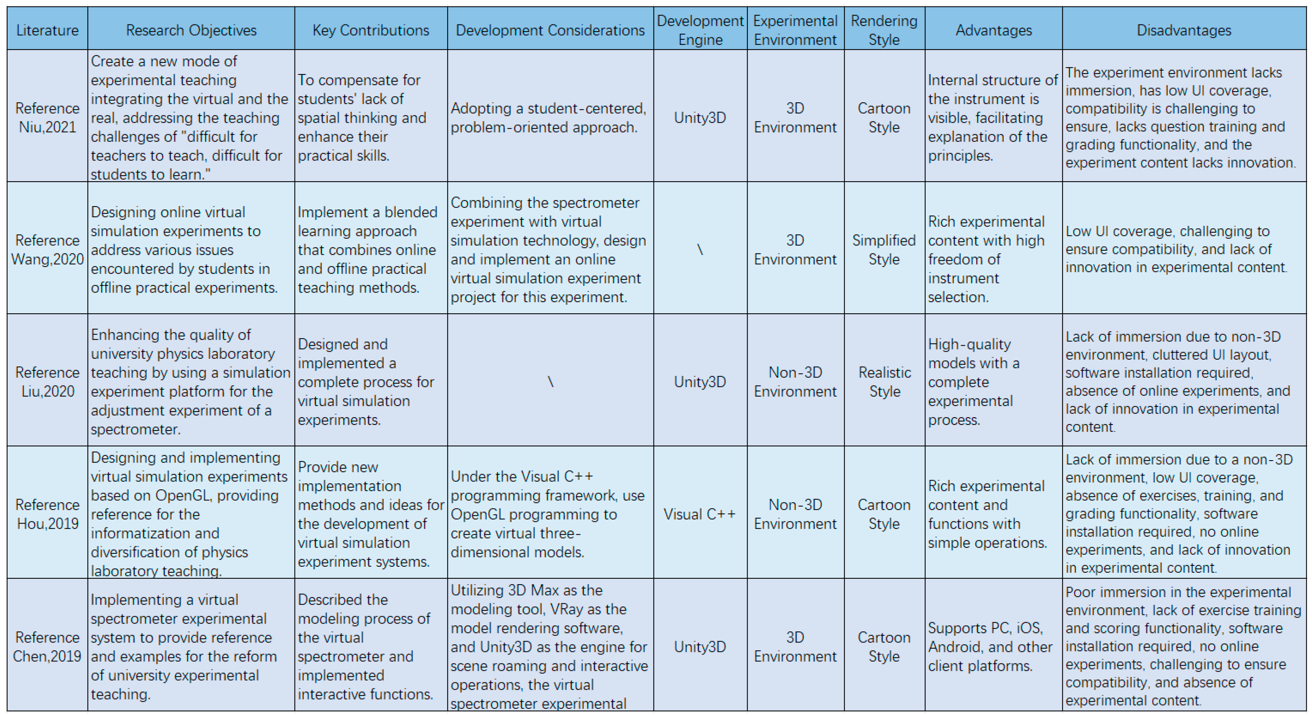
1.2. Related Research

With the continuous updates and iterations of virtual simulation technology, the application of simulated experiments in experimental teaching represents a new avenue of exploration in education. Numerous studies and practical achievements have been gained through extensive research on virtual simulation experiments in domestic universities and enterprises. The optical physics simulation system related to the spectrometer, as shown in Figure 1, is introduced below.

In the work by [8], a virtual system for a spectrophotometer physics experiment is developed using Unity 3D. This system exhibits the internal and external structures as well as principles of the instrument in a three-dimensional virtual space, characterized by ease of learning, usability, and advanced features. However, the experimental instruments in this virtual system lean towards a cartoon style and lack UI interface displays and experimental grading functions. The virtual simulation experiment project on spectrophotometry presented in [9] includes multiple teaching contents, achieving the integrated cultivation of basic skills and inquiry-based learning. Nevertheless, this virtual simulation experiment project has a relatively limited number of UI windows and lacks experimental result displays. In [10], a spectrophotometer simulation experiment platform is introduced with rich UI windows and a complete experimental process. However, this simulation experiment is not conducted in a three-dimensional virtual space, and the UI layout is complex. Additionally, the use of this simulation experiment platform requires the configuration of corresponding environments and the installation of specific plugins, making it somewhat cumbersome. Meanwhile, ref. [11] designs multiple spectrophotometer virtual simulation experiments using OpenGL programming, suitable for experiment explanations to enhance students’ interest in and enthusiasm for learning. Nevertheless, the interface of this virtual simulation experiment is relatively rudimentary, the material of the experimental instruments is distorted, and it lacks an experimental grading function. In [12], a spectrophotometer virtual experiment developed using Unity 3D is highlighted for its simple operation, user-friendly interface, and cross-platform operation. However, the virtual experiment scene is rudimentary, and the content and functional options are insufficient.

In summary, in most virtual simulation platforms, due to the desire to shorten the development cycle and reduce development costs, the following four problems exist in the developed simulation systems.

(1)

The experimental process is fixed and singular, and students can only mechanically complete the required experimental operations, reducing the opportunities for students’ independent exploration of experiments.

(2)

The use of virtual simulation programs requires the installation of cumbersome auxiliary software or plugins, leading to compatibility risks when used across platforms, limiting the user base and system promotion.

(3)

The system’s immersion and experience are not ideal, and the experimental environment and instruments are non-3D models, making it difficult for students to interact well with the experimental instruments and understand their structure and principles. The low-coverage UI interface and additional operation introductions increase the learning burden on students, causing them to develop feelings of frustration [13].

(4)

The system’s use requires a significant amount of computer resources, making it difficult for low-performance computers to run smoothly when other programs are running in the background.

Ultimately, these issues make virtual simulation experiments unable to meet the current teaching needs.

1.3. Our Research

After an extensive literature review and firsthand experience with virtual spectrophotometer simulation programs, the identified issues are summarized and analyzed. To address these challenges, this paper proposes a design method for an optical physics virtual simulation system based on Unreal Engine 5. This involves using Unreal Engine 5 as the development engine, employing a generic design architecture to divide subsystems, and adopting mature technologies such as pixel streaming and physics engines as the development approach for the virtual simulation system. The goal is to design and implement a realistic 3D virtual experimental environment. To address the existing issues with simulation systems, the effectiveness of the research method is as detailed below.

(1)

To address the issue of a fixed and singular experimental process, the system integrates the spectrometer’s grating diffraction experimental system and presents it in a step-by-step experimental format. Students can autonomously design experimental solutions to meet specific requirements for practical problems, fostering students’ experimental innovative thinking abilities, ensuring satisfaction, and enhancing students’ willingness to use it [14]. This lays a solid experimental foundation for subsequent course learning and work.

(2)

To tackle compatibility issues, the system utilizes the pixel streaming technology solution of Unreal Engine 5. Users can smoothly use the virtual simulation system without the need for software or plugin installations, thereby resolving compatibility issues when used across platforms.

(3)

To address the issues of immersion and experience in the system, this virtual simulation system employs SolidWorks to create high-precision 3D models. It utilizes the LUMEN and NANITE technologies of the Unreal Engine 5 engine to achieve the real-time rendering of dynamic scenes, making the experimental scenes of the virtual simulation system more delicate and realistic. Additionally, the system creates a UI interface with higher coverage and simplicity, and the principles and theoretical explanations of the experiments are presented mostly through animated videos. The personalized design of experiments, sound effects, UI design, function buttons, etc., significantly increase students’ interest in learning and reduce the learning cost of using the program. However, high-precision models may occupy more computer hard drive space.

(4)

To address performance issues, the system adopts a web-based access method. The program’s operation does not consume computer resources, and users can directly perform experimental operations by entering a URL, greatly reducing the computer performance requirements for users.

This study provides a strong reference for the further development of virtual experimental systems and offers valuable insights into the future direction of physics experimental teaching. Finally, the article uses a comparative approach to demonstrate the effectiveness of the method and the superiority of the system.

2. System Design Principles

2.1. Unreal Engine 5

Unreal Engine is a robust game engine developed by Epic Games, utilized to create high-quality 3D games and simulation applications. Widely employed in game development, virtual reality (VR), augmented reality (AR), film production, and other real-time interactive application developments, it has found extensive application in the fields of simulation and emulation [15,16,17,18,19,20,21,22,23].

This engine not only offers advanced graphic technologies but also facilitates more intuitive game development through tools like the Blueprint system. Key technologies within the engine include the graphics engine (encompassing advanced rendering techniques such as physics-based rendering, global illumination, real-time shadows, and reflections, this engine enables games and applications to present visually stunning effects); the Blueprint system (utilizing a graphical programming approach, this system allows non-programmers to rapidly create complex game systems by dragging and connecting different nodes, eliminating the need for coding); and scalability (developers can customize and extend the engine’s functionality through a plugin system, meeting specific development requirements).

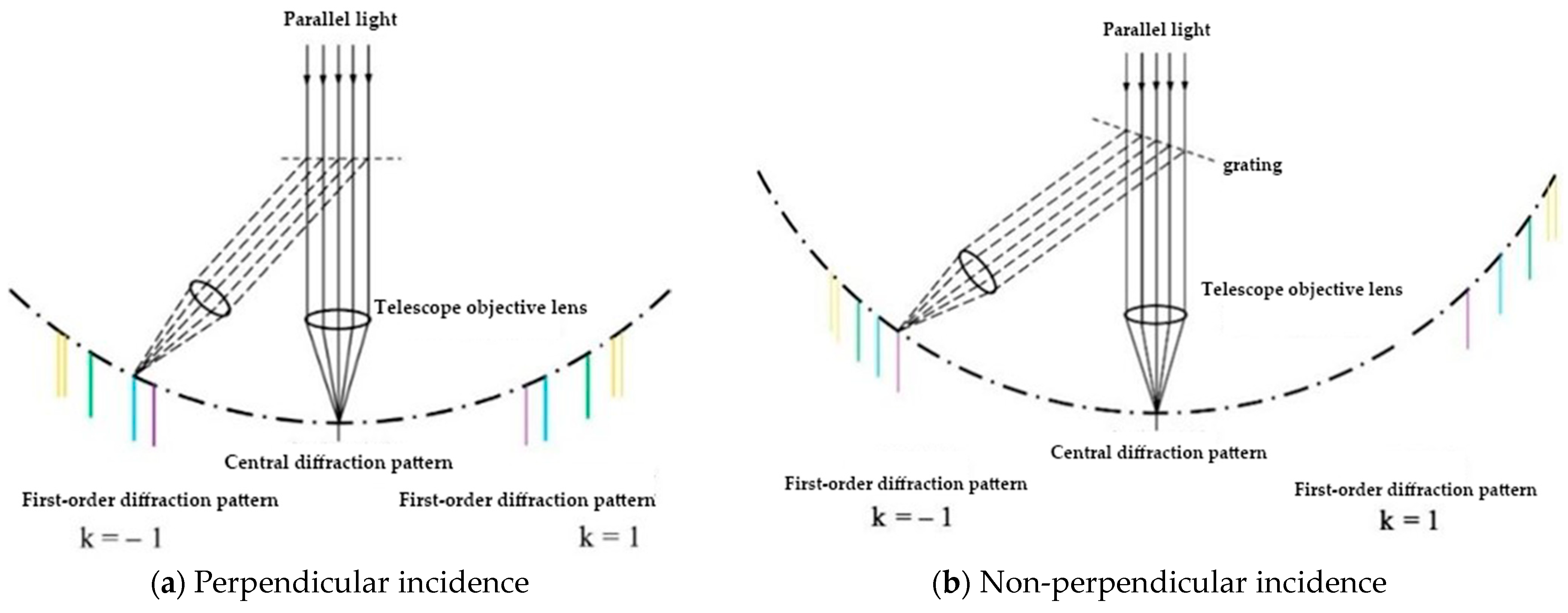
2.2. Principles of Optical Experiments

In reference to the teaching objectives of the “University Physics Laboratory” course, the virtual simulation system is designed to encompass experimental aspects of optical physics, including spectrophotometer adjustment, non-perpendicular incident grating diffraction, and equal-inclination grating diffraction. The principles of these experiments are outlined as follows.

Initially, when light is incident perpendicularly on a grating, according to the diffraction theory of gratings, the positions of the bright fringes in the diffraction spectrum are determined by the following equation:

$$d\mathit{sin}{\phi }_k=\pm k\lambda$$

(1)

where $d$ represents the grating constant, $\lambda$ is the wavelength of the incident light, $k$ denotes the order of the bright fringe (spectral line), and ${\phi }_k$ signifies the diffraction angle of the $k$-order bright fringe.

If the incident light is polychromatic, different wavelengths will result in distinct diffraction angles ${\phi }_k$, leading to the dispersion of the polychromatic light. At the central point ($k=0$, ${\phi }_k=0$), all colors overlap to form the central bright fringe. Symmetrically distributed on either side of the central bright fringe ($k=0$) are spectral lines for $k=0, 1, 2, 3, \cdot \cdot \cdot$. These spectral lines are arranged in order of increasing wavelength, forming a spectrum known as the grating spectrum, as illustrated in Figure 2a.

Subsequently, when the grating plane is rotated from a state of perpendicular incidence with an angle $i$ (where $i$ is the angle of parallel light incidence), the diffraction angle is defined as the angle between the diffracted light and the 0th-order spectrum. According to grating diffraction theory, the formula for non-perpendicular incidence is as follows:

$$d\mathit{sin}({\phi }_k-i)+d\mathit{sin}i=\pm k\lambda ,(k=0,1,2,\dots )$$

(2)

where $d$ represents the grating constant, $\lambda$ is the wavelength of the incident light, $k$ denotes the order of the bright fringe (spectral line), ${\phi }_k$ signifies the diffraction angle of the $k$-order bright fringe, and $i$ is the angle of incidence of the light ray.

Finally, when the incident light and diffracted light are on the same side, for green light with a known wavelength $\lambda$ incident at an angle $i$ on the grating, satisfying Formula (2), it is evident that the diffraction angle ${\phi }_k$ varies with the change in $i$. Through mathematical methods, it is not difficult to prove that when ${\phi }_k=2i$, ${\phi }_k$ has a minimum value, known as the minimum diffraction angle (${\phi }_{min}$). Importantly, the minimum diffraction angle occurs only when the incident and diffracted light are on the same side. Therefore, substituting ${\phi }_{min}$ into the formula,

$$d=\frac{k\lambda }{2\mathit{sin}(\frac{{\phi }_{min}}{2})},\left(k=\mathrm{0,1},2,\dots \right)$$

(3)

where $\lambda$ is the wavelength of green light. By measuring ${\phi }_{min}$, the grating constant $d$ can be determined.

When implementing the virtual simulation system, considering the issue of performance optimization, the simulation of grating diffraction is displayed in the UI window at the bottom left corner. The display function of this window is equivalent to the observation function of the eyepiece in the real-world spectrometer. The simulation method presents diffraction spectra in different colors as images. When adjusting the experimental components, the position, rotation, transparency, width, and narrowness of the images in the UI window are adjusted by the formulas and algorithms based on the physical principles, achieving the simulation of diffraction patterns.

When investigating the physical mechanism behind the virtual circular diffraction pattern generation, the green electronic screen allows the selection of grating types (600-line grating, 300-line grating) and laser colors (green laser 532 nm, violet laser 405 nm, red laser 666 nm). By modifying the grating type and laser color, the parameter information in the formula is changed, ultimately producing diverse circular diffraction patterns. In other words, the variation in the grating diffraction pattern is determined by the parameters input into the formula.

3. General System Design

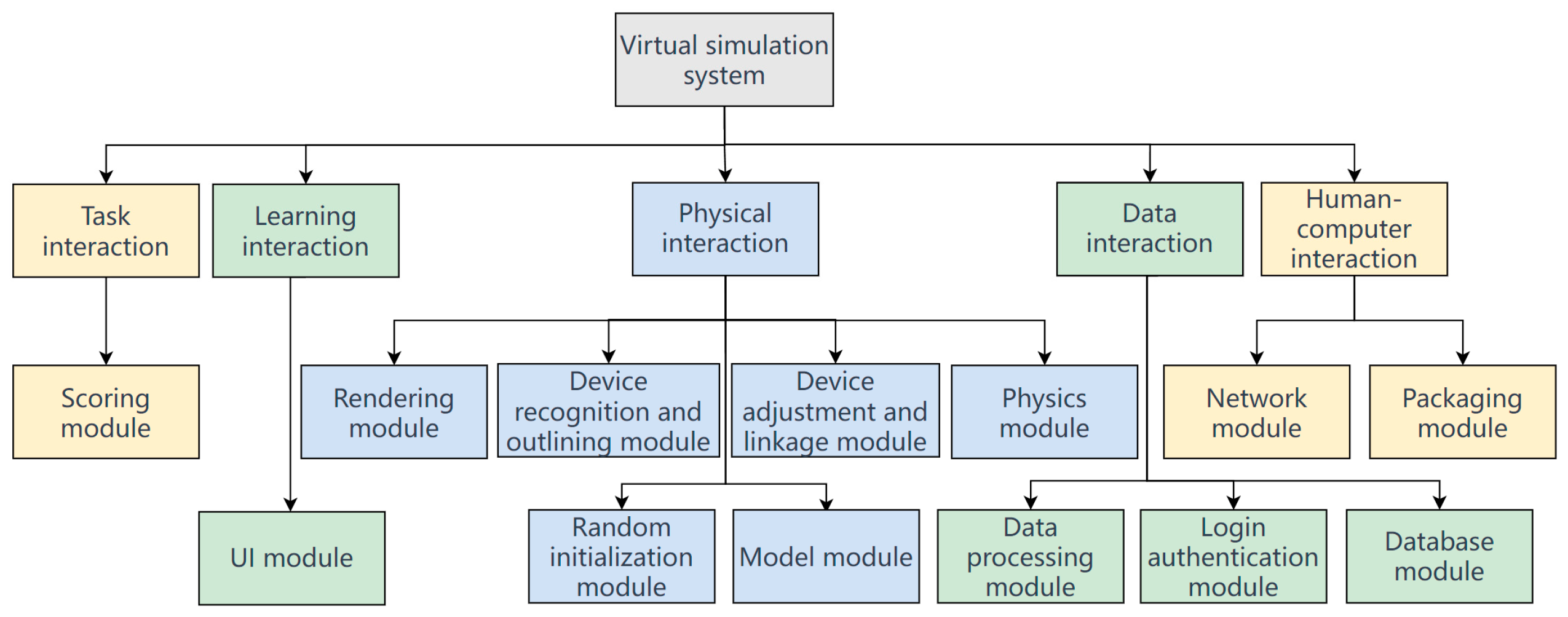
3.1. Overall Design

The diversity of experimental phenomena can be attributed to variations in parameters within the physics formulas. Therefore, the system is founded on the principles of experimental physics, incorporating the latest virtual simulation technologies [24]. Multiple experiments within this virtual simulation system adhere to a generic design architecture. Based on the interactive nature of virtual reality, the system is divided into five subsystems, as illustrated in Figure 3: Task Interaction, Learning Interaction, Physical Interaction, Data Interaction, and Human–Computer Interaction.

(1)

The Physical Interaction subsystem implements the experimental operation and scene rendering functions of virtual simulation. It enhances the system reusability and immersion. When integrating new experimental content, each module’s functionality can be reused, reducing the development cycles and costs while maintaining a detailed and realistic experimental environment with consistent operating methods. After starting the experiment, the initial state values of the experimental instruments will be randomly processed, providing the most intuitive feedback through changes in optical phenomena by adjusting the spatial information and relevant physical parameters using the operation adjuster.

(2)

The Learning Interaction subsystem implements UI functions such as phenomenon observation, data measurement, and recording. It enhances the system scalability, and, by adding other teaching materials, the relevant functions of this subsystem can be reused, facilitating the addition of subsequent experiments and avoiding the rigidification of experiments. The visual drag-and-drop window allows the convenient observation of the physical space changes of the devices without adjusting one’s position and perspective.

(3)

The Data Interaction subsystem implements functions such as data storage and information processing, enhancing the system’s management and maintenance capabilities for experimental data resources. This subsystem processes the physical data generated by adjusting instruments based on the algorithms in the experimental principles. It achieves the localized storage and retrieval of information through MySQL Integration plugin technology, facilitating teachers and students in viewing experimental data, teaching materials, and grade rankings.

(4)

The Task Interaction subsystem implements functions for the evaluation and querying of grades, enhancing the system’s practicality. The system automatically grades the experiment at the end, allowing students to repeat the experiment to achieve better grades. The entire process does not require teacher involvement, reducing the workload of supervision and grading.

(5)

The Human–Machine Interaction subsystem implements the local and network usage of the program, improving the system compatibility and reducing the computer performance requirements. By providing a “.exe” executable program directly through the packaging module, the local program’s real-time rendering will occupy some computer resources, requiring a computer with better performance. The network module uses pixel streaming technology, allowing direct access and usage of the simulation system through a webpage, without installing any software or plugins.

3.2. Module Introduction

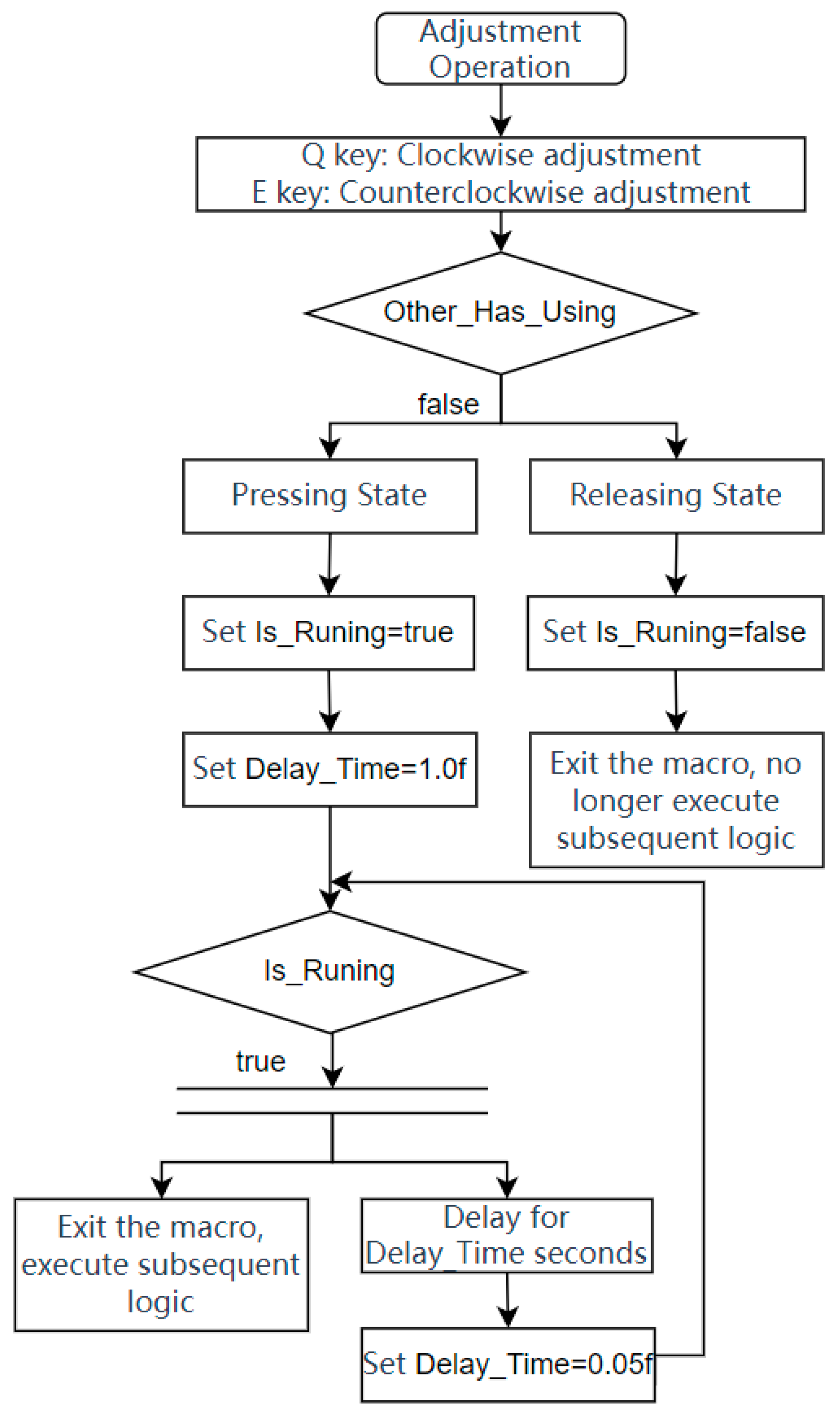
3.2.1. Device Adjustment and Linkage Module

(1)

Device Adjustment:

Device adjustment is divided into two types: single adjustment and continuous adjustment. Single adjustment is used for fine-tuning, while continuous adjustment is employed for coarse adjustments. By measuring the physical linkage brought about by the movement of each component of the spectrometer, and utilizing Unreal Engine 5 to store all measured engineering parameters in variables, the adjustment functionality is implemented through blueprint scripting. The ultimate goal is to achieve dynamic effects close to the real world.

(2)

Device Linkage:

Device linkage primarily consists of five types: single device rotational motion, single device translational motion, single device combined rotational and translational motion, multi-device rotational linkage, and multi-device rotational and translational linkage.

Since device motions are classified into rotation and translation, the system only needs to implement the functionality of these two motion types in the top-level parent class of the instrument. However, constant attention to the moving objects is necessary, as, in the case of multi-device linkage, it involves other object devices. Hence, their parent–child relationships are particularly important (the child in the physical space will adhere to the parent’s movement).

Below is the algorithmic content of this module. First, let us declare the meanings of the variables:

(1)

Boolean variable ‘Other_Has_Using’ indicates whether other keys are invoking the macro. It is set to false only when the conditions “(pressing Q key and releasing E key) or (pressing E key and releasing Q key)” are satisfied.

(2)

Boolean variable ‘Is_Runing’ represents whether the macro is currently running. It is set to true only when the macro is running.

(3)

Floating-point variable ‘Delay_Time’ represents the delay time.

As shown in Figure 4, when invoking the macro, it is necessary to first check whether other keys are invoking the macro. The execution continues only when “Other_Has_Using == false”. When the key status is released, we set “Is_Runing == false” to indicate that the macro is not running. After exiting the macro, subsequent logic is not executed. When the key status is pressed, we set “Is_Runing == true” to indicate that the macro is running. At this point, the first delay time ‘Delay_Time’ is set to 1 s. Then, the initial judgment of ‘Is_Runing‘ is executed. When “Is_Runing == true”, we exit the macro concurrently, execute subsequent logic, and delay for ‘Delay_Time’ time. The first delay is 1 s, and, during this period, releasing the key results in a single adjustment. If the pressing time exceeds 1 s, it becomes a continuous adjustment. Under continuous adjustment, we set a new delay time ‘Delay_Time’ to 0.05 s. This allows the continuous checking of the ‘Is_Runing’ state and the execution of subsequent logic.

3.2.2. Physics Module

In this virtual simulation system, the Physics module comprises two main components. One part involves custom physics effects, as mentioned earlier, such as device adjustment and linkage. The other part utilizes the engine’s built-in physics simulation, specifically the Chaos Physics Engine, capable of collision detection, object movement, and deformation simulation. When adjusting the leveling screw of the specimen stage, there are changes in tilt and displacement, constituting a complex linkage problem. Therefore, the engine’s physics simulation is employed to assist in system development. However, due to factors such as friction and gravity, the specimen stage is not in a state of strict constraint relative to the cursor disc. Therefore, additional physical constraints need to be added to account for these influences.

3.2.3. Rendering Module

The quality of rendering directly impacts the realism of the simulation. This simulation system leverages the NANITE and LUMEN technologies of Unreal Engine 5, both of which deliver stunning visual effects.

In the laboratory setting, numerous experimental instruments feature high-precision models, resulting in a vast number of polygons in the scene’s mesh. Through the utilization of Nanite and virtual shadow mapping techniques, only the perceptible details are streamed and processed. This significantly alleviates the limitations on polygon counts and draw calls, ensuring a stable runtime frame rate.

LUMEN technology provides a fully dynamic global illumination and reflection solution, allowing real-time adjustments to indirect lighting. Consequently, while manipulating experimental instruments, users can clearly observe the real-time changes in indoor lighting and shadows.

3.2.4. Scoring Module

This module is implemented through user control blueprints and an event dispatcher. The scoring criteria are defined based on the course requirements. The module assesses user performance comprehensively, considering the parameters of device adjustments, the sequence of device adjustments, and recorded data values.

The scoring is particularly influenced by the comparison between recorded data values, provided by the user, and standard range values. For instance, during fine-tuning, adjusting the green crosshair to the corresponding position would earn a full score if the deviation is less than 0.04 mm. Conversely, a deviation exceeding 0.1 mm would result in a zero score, and proportional scores within the range of 0.04 mm to 0.1 mm would be assigned accordingly.

$$\mathrm{A}=(0.1 \mathrm{m}\mathrm{m}-\mathrm{B})÷(0.1 \mathrm{m}\mathrm{m}-0.04 \mathrm{m}\mathrm{m})\times \mathrm{C}$$

(4)

where $\mathrm{A}$ represents the final score, $\mathrm{B}$ denotes the measured experimental error, and $\mathrm{C}$ represents the maximum achievable score.

3.2.5. UI Module

In this virtual simulation system, the UI is primarily divided into two categories: the functional UI and view UI.

The functional UI includes the menu bar, grade inquiry, numerical measurement, data calculation, table filling, website access, and touchscreen functionality. For instance, through the touchscreen, students can configure the grating type and laser color. Once the correct optical phenomenon occurs, students can use the numerical measurement UI to place the goniometer in the desired position, measure the values of the required data, record them in the table filling UI, and finally obtain the settlement results by clicking the “Calculate” button in the data calculation UI.

The view UI comprises visual drag-and-drop windows, experiment introductions, principle explanations, and device introductions, designed for viewing and exploring specific experimental content. Utilizing the Web Browser plugin technology enables web-based access, facilitating the expansion of related theoretical knowledge learning and enhancing system interactivity and user experience. In this simulation system, a total of 12 visual drag-and-drop windows are employed to allow operators to see views from specific angles during the experimental operation, avoiding frequent adjustments of the position and angle to observe phenomena. Additionally, visual drag-and-drop windows can be freely placed according to the requirements (as shown in Figure 5).

3.2.6. Network Module

This module primarily utilizes the Pixel Streaming technology of Unreal Engine 5. The Pixel Streaming plugin allows the direct streaming of rendered visual 3D graphics content and audio information to browsers and mobile devices.

When enabling the Pixel Streaming plugin, we package the project using the “Windows + Shipping” method. After packaging is complete, we create a copy of the “.exe” program file and append the following parameters at the end of the “Target” box in the file properties: “-AudioMixer -RenderOffScreen -PixelStreamingIP=localhost -PixelStreamingPort=6666 NvEncH264ConfigLevel=NV_ENC_LEVEL_H264_52”.

Next, we execute the “Start_SignallingServer.ps1” file to initiate the signaling server. The first run will automatically deploy the necessary environment. After completing these steps, we can access the system locally in a web browser using the address “http://127.0.0.1/ (accessed on 10 August 2023)”. Utilizing DDNSTO’s domain mapping technology allows for public network access.

4. Experiment Process

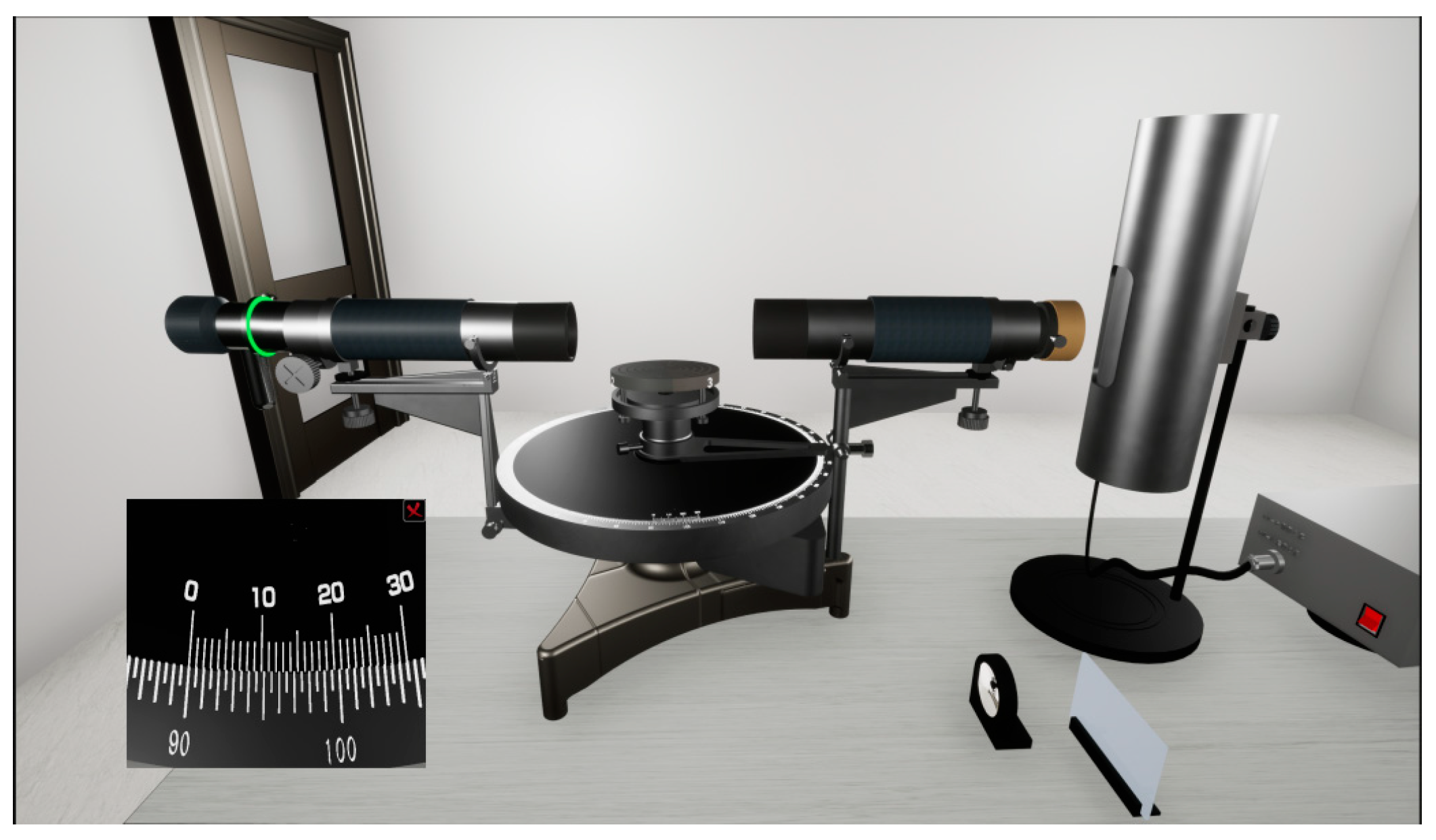
4.1. Experimental Operation

A virtual laboratory serves not only as a digitized space but also as an extension of real-world operations. Whether rotating experimental devices or observing optical phenomena, each action feels as if one is in a physical laboratory, providing a strong sense of immersion. Below are the brief steps for the operation of instruments in the simulated experiment:

(1)

Adjustment of Telescope for Parallel Light Reception. Utilize methods such as the self-collimation method, rough adjustment method, and semi-adjustment method to ensure that the telescope receives parallel light.

(2)

Adjustment of Collimator to Emit Parallel Light. Utilize the properly adjusted telescope to adjust the collimator, ensuring that it emits parallel light.

(3)

Placement of Grating and Alignment. Place the diffraction grating and rotate the vernier disc to align the green crosshair in the telescope with the central bright fringe. Secure relevant screws after alignment.

(4)

Observation of ±1 Order Spectra. Read the angular coordinates of the central bright fringe at this point. Rotate the telescope to observe the ±1 order spectra on both sides. Adjust the screws to make both side spectra of equal height.

(5)

Adjustment of Carrier Stage and Data Collection. Unlock the screws of the carrier stage, rotate it, and observe the movement of the spectra. Simultaneously observe the minimum diffraction angle and disappearance point. Record and analyze data accordingly.

These steps ensure a systematic approach to the virtual experiment, providing a simulated but immersive experience akin to performing the same actions in a physical laboratory.

4.2. Data Recording

To minimize measurement errors when determining the minimum diffraction angle for green light [25], the following method is employed.

Setting the Reference Point. Use the normal to the grating as a reference. When the incident light and diffracted light are on the same side of this reference, proceed to the next steps.

Finding +1 Order Diffraction. Release and rotate the specimen stage until the +1 order green light diffraction angle is minimized. Fix the stage in this position and measure the coordinate of the +1 order green light spectrum angle at this point.

Finding −1 Order Diffraction. Release and rotate the specimen stage again, this time aligning the normal to the grating plane near the symmetrical position. Locate the position where the −1 order green light diffraction angle is minimized. Fix the stage and record the coordinate of the −1 order green light spectrum angle.

Calculating Minimum Diffraction Angle. Calculate the minimum diffraction angle ${\phi }_{\mathrm{m}\mathrm{i}\mathrm{n}}$ and the corresponding incident angle $i_{\mathrm{m}\mathrm{i}\mathrm{n}}$ for green light. Determine the grating constant $d$ using the measured angles, As shown in

Table 1. Measurement of minimum deflection angle.

$\mathit{K}=1$ Spectral Coordinates		$\mathit{K}=-1$ Spectral Coordinates		${\mathit{\phi }}_{\mathbf{m}\mathbf{i}\mathbf{n}}$	${\mathit{i}}_{\mathbf{m}\mathbf{i}\mathbf{n}}$
$\mathbf{Left} {\mathit{\theta }}_1$	$\mathbf{Right} {\mathit{\theta }}_1^{\mathit{’}}$	$\mathbf{Left} {\mathit{\theta }}_{-1}$	$\mathbf{Right} {\mathit{\theta }}_{-1}^{\mathit{’}}$
$284°{56}^{\prime }$	$104°{56}^{\prime }$	$322°{37}^{\prime }$	$142°{38}^{\prime }$	$18°{51}^{\prime }$	$9°{25}^{\prime }$

.

Minimum diffraction angle

$${\phi }_{\mathrm{m}\mathrm{i}\mathrm{n}}=\frac{1}{4}\left(\right|{\theta }_1-{\theta }_{-1}|+|{\theta }_1^{\prime }-{\theta }_{-1}^{\prime }\left|\right)$$

(5)

Incident angle corresponding to the minimum deflection angle

$$i_{\mathrm{m}\mathrm{i}\mathrm{n}}=\frac{{\phi }_{\mathrm{m}\mathrm{i}\mathrm{n}}}{2}$$

(6)

The formula includes the following parameters. ${\phi }_{min}$: minimum diffraction angle for green light. $i_{min}$: incident angle corresponding to the minimum deviation angle. $k$: order of the bright fringe (spectral line). ${\theta }_1$: angle of the left cursor for the 1st diffraction order of green light. ${\theta }_1^{\prime }$: angle of the right cursor for the 1st diffraction order of green light. ${\theta }_{-1}$: angle of the left cursor for the −1st diffraction order of green light. ${\theta }_{-1}^{\prime }$: angle of the right cursor for the −1st diffraction order of green light.

Next, measuring the diffraction angles at different incident angles involves a sequence of steps [26]. Begin by rotating the telescope to align the central bright fringe with the vertical crosshair. Lock the telescope in place and release the stage’s locking screw, allowing it to rotate until the green crosshair aligns vertically with the central bright fringe. Secure the stage and record the angle coordinates of the central bright fringe. Fix the telescope, release the stop screw of the graduated disc, and rotate the disc to introduce an angle $i$ between the incident light and the normal. Lock the disc in place and read the angle coordinates of the central bright fringe. Finally, release the telescope and measure the angle coordinates of the ±1 order green light. Finally, obtain $\overline{{\phi }_{+1}}\left(i\right)$ and $\overline{{\phi }_{-1}}\left(i\right)$ based on the following formula and record them in

Table 2. Calculation of measured and theoretical values of green light diffraction angles.

n	$\mathit{i}\left(\mathit{n}\right)$	$\overline{{\mathit{\phi }}_{+1}}\left(\mathit{i}\right)$	${\mathit{\phi }}_{+1, \mathbf{T}\mathbf{h}\mathbf{e}\mathbf{o}\mathbf{r}\mathbf{y}}\left(\mathit{i}\right)$	$\overline{{\mathit{\phi }}_{-1}}\left(\mathit{i}\right)$	${\mathit{\phi }}_{-1, \mathbf{T}\mathbf{h}\mathbf{e}\mathbf{o}\mathbf{r}\mathbf{y}}\left(\mathit{i}\right)$
0	$0°0^{\prime }$	$19°{07}^{\prime }$	$19°{08}^{\prime }$	$19°{07}^{\prime }$	$19°{08}^{\prime }$
1	$9°{25}^{\prime }$	$18°{54}^{\prime }$	$18°{52}^{\prime }$	$19°{57}^{\prime }$	$20°0^{\prime }$
2	$20°0^{\prime }$	$19°{10}^{\prime }$	$19°{11}^{\prime }$	$22°{03}^{\prime }$	$22°{03}^{\prime }$
3	$31°0^{\prime }$	$20°{12}^{\prime }$	$20°{12}^{\prime }$	$26°{28}^{\prime }$	$26°{26}^{\prime }$
4	$40°0^{\prime }$	$21°{38}^{\prime }$	$21°{38}^{\prime }$	$36°{05}^{\prime }$	$36°{02}^{\prime }$
5	$45°0^{\prime }$	$22°{43}^{\prime }$	$22°{42}^{\prime }$	/	/
6	$55°0^{\prime }$	$25°{34}^{\prime }$	$25°{34}^{\prime }$	/	/
7	$65°0^{\prime }$	$29°{38}^{\prime }$	$29°{39}^{\prime }$	/	/
8	$75°0^{\prime }$	$35°{21}^{\prime }$	$35°{20}^{\prime }$	/	/
9	$85°0^{\prime }$	$43°{03}^{\prime }$	$43°{03}^{\prime }$	/	/

.

The formula for the angle of incidence is as follows:

$$i\left(n\right)=\frac{1}{2}(\left|{\theta }_0\left(n\right)-{\theta }_0\left(0\right)\right|+\left|{\theta }_0^{\prime }\left(n\right)-{\theta }_0^{\prime }\left(0\right)\right|)$$

(7)

The formula for the +1st order diffraction angle is given by

$$\overline{{\phi }_{+1}}\left(i\right)=\frac{1}{2}(\left|{\theta }_1\left(n\right)-{\theta }_0\left(n\right)\right|+\left|{\theta }_1^{\prime }\left(n\right)-{\theta }_0^{\prime }\left(n\right)\right|)$$

(8)

The formula for the −1st order diffraction angle is as follows:

$$\overline{{\phi }_{-1}}\left(i\right)=\frac{1}{2}\left(\right|{\theta }_{-1}\left(n\right)-{\theta }_0\left(n\right)|+|{\theta }_{-1}^{\prime }\left(n\right)-{\theta }_0^{\prime }\left(n\right)\left|\right)$$

(9)

The formula includes the following variables. $i\left(n\right)$: incidence angle with index $n$. ${\theta }_0\left(n\right)$: left cursor degree of the 0th order diffraction of green light with index $n$. ${\theta }_0^{\prime }\left(n\right)$: right cursor degree of the 0th order diffraction of green light with index $n$. ${\theta }_1\left(n\right)$: left cursor degree of the 1st order diffraction of green light with index $n$. ${\theta }_1^{\prime }\left(n\right)$: right cursor degree of the 1st order diffraction of green light with index $n$. ${\theta }_{-1}\left(n\right)$: left cursor degree of the −1st order diffraction of green light with index $n$. ${\theta }_{-1}^{\prime }\left(n\right)$: right cursor degree of the −1st order diffraction of green light with index $n$.

4.3. Data Processing and Analysis

(1)

Given the wavelength of mercury lamp green light as 546.1 nm, the calculation for the minimum diffraction angle and the results for the incidence angle are as follows:

$$i_{\min }=\frac{{\phi }_{\min }}{2}=\frac{18°50^{\prime }}{2}=9°{25}^{\prime }$$

(10)

The calculation results for the grating constant are as follows:

$$d=\frac{k\lambda }{2\mathit{sin}(\frac{{\phi }_{\min }}{2})}{=\frac{546.1\times 10^{-6}\mathrm{mm}}{2\mathit{sin}(\frac{18°50^{\prime }}{2})}=1.669\times 10}^{-3}\left(\mathrm{mm}\right)$$

(11)

The formula includes the following variables. ${\phi }_{min}$: minimum diffraction angle for green light. $i_{min}$: corresponding angle of minimum deviation. $k$: bright fringe (spectral line) order. $d$: grating constant. $\lambda$: wavelength of incident light.

(2)

Calculate the measured and theoretical values of green light diffraction angles at different incident angles.

$${\phi }_k=\mathit{arcsin}(\frac{k\lambda }{d}-\mathit{sin}i)+i,\hspace{0.33em}\hspace{0.33em}(k=\pm 1)$$

(12)

The formula includes ${\phi }_k$, the diffraction angle of the $k$-th bright fringe; $i$, the angle of incidence of the light; $k$, the order of the bright fringe (spectral line); $d$, the grating constant; $\lambda$, the wavelength of the incident light.

(3)

Draw the graph depicting the relationship between the green light diffraction angles and incident angles, as shown in Figure 6.

5. Innovation and Advantage

The virtual simulation system, developed through Unreal Engine 5, not only measures high-precision physical data but also reflects real-world experimental errors. Regardless of how the experimental instruments are operated, the observed phenomena and measured values closely align with the real world. The following will demonstrate the superiority of the system and the feasibility of the approach through a comparative analysis.

(1)

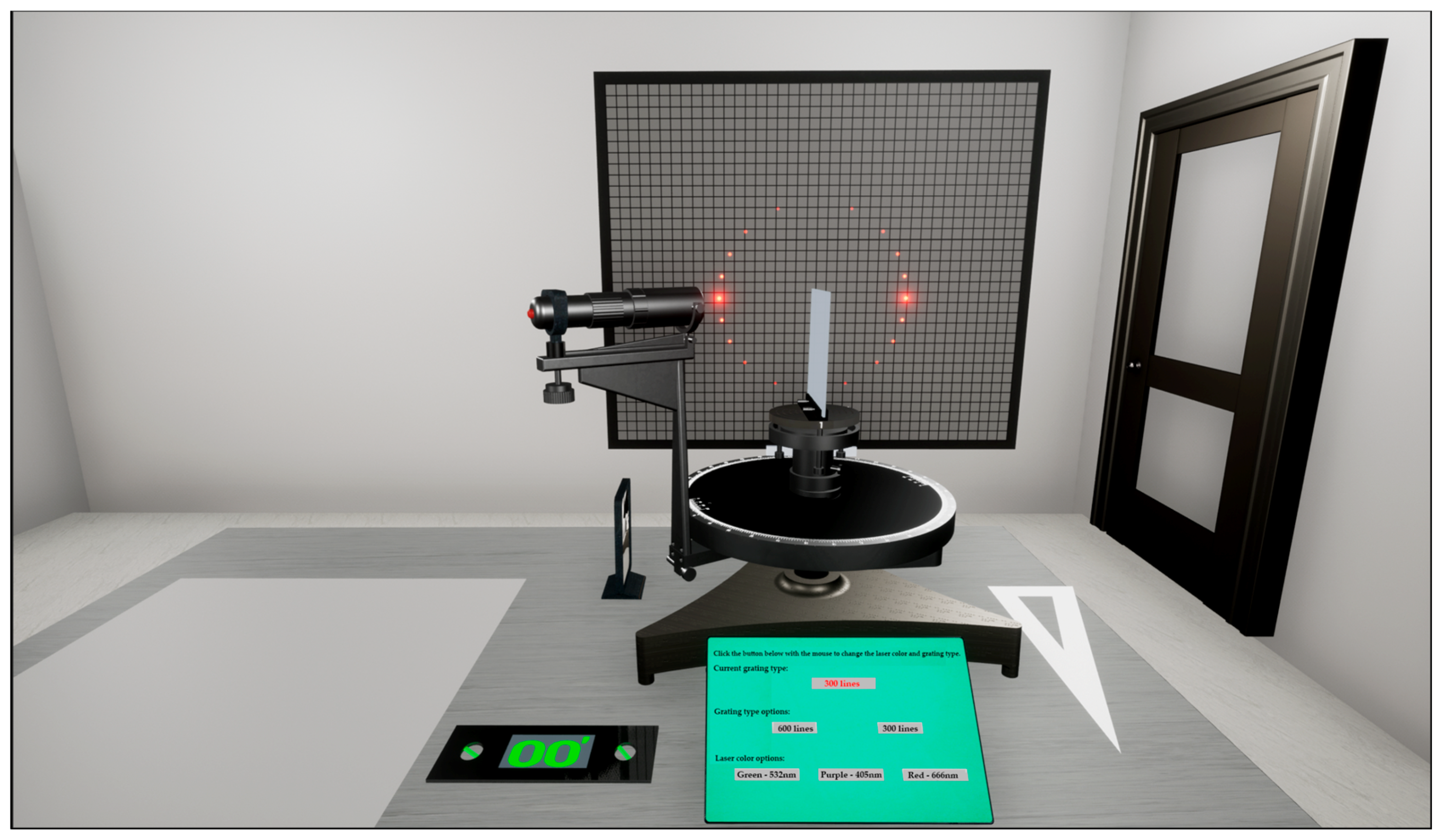
The experimental content is innovative. The studies in [8,9,10,11,12] do not innovate the experimental content of the spectrometer. However, the virtual simulation experiments in this system include self-designed experiments (as shown in Figure 7). The grating equal inclination instrument used in the experiment is also a homemade device (replacing the telescope of a discarded spectrometer with a laser, transforming the parallel light tube into a receiving screen, and keeping other parts unchanged). Independently exploring innovative experiments can better cultivate students’ practical and innovative abilities.

(2)

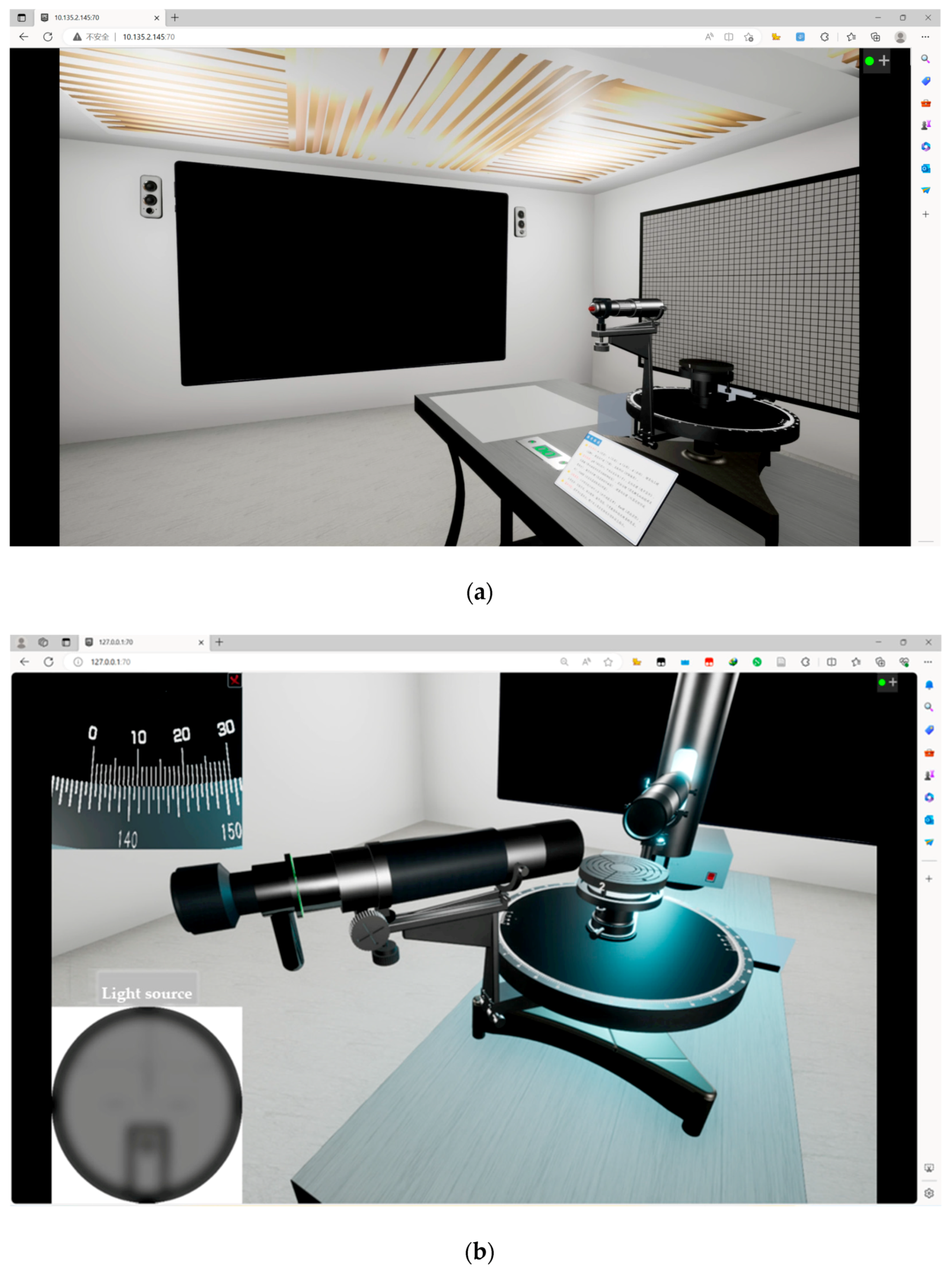
Compatibility and cross-platform use are enhanced in this simulation system. Unlike the simulation programs in references [10,12], which only provide .exe files, our simulation system includes both a local version and a web version. The information between the program and the webpage is synchronized in real time through a database. The web version can run the program directly without installing any software or plugins (as shown in Figure 8), avoiding compatibility issues across different computer systems.

(3)

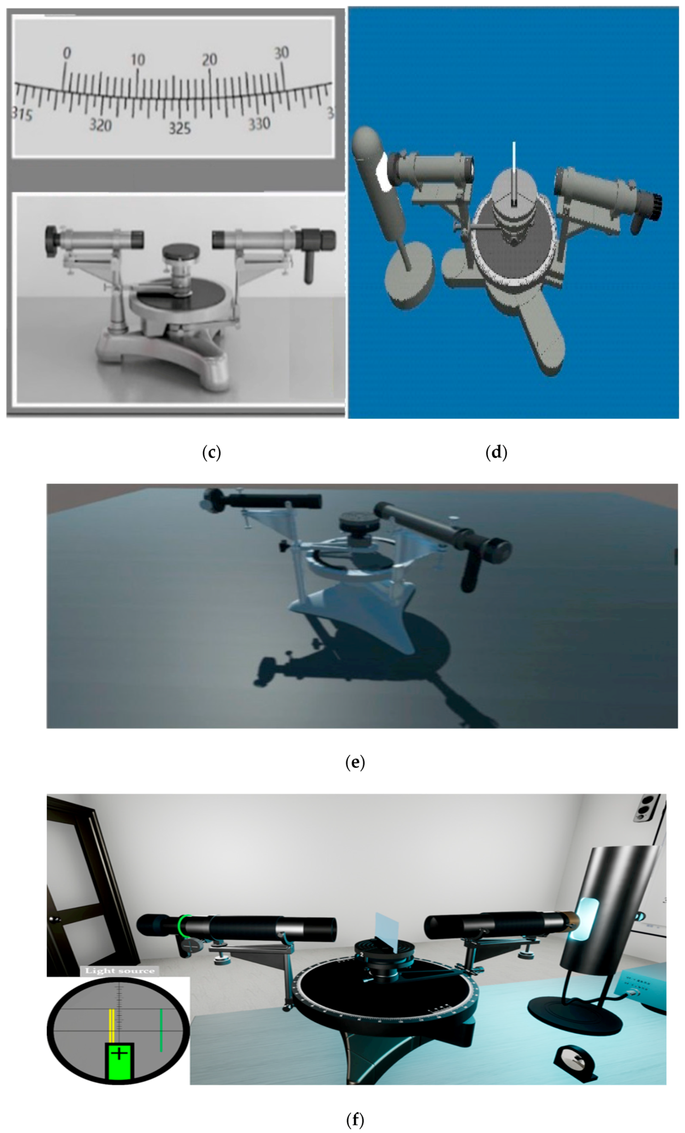
A strong sense of immersion. Comparing the virtual experiments using the virtual spectrometer in this article with those in references [8,9,10,11,12], the actual effect is shown in Figure 9. It can be visually perceived that the immersion of the spectrometer experiment based on Unreal Engine 5 (Figure 9f) is stronger. The model’s texture and material gloss are of higher quality, and users in such a high-quality virtual laboratory can greatly avoid the operational dissonance caused by mouse and keyboard operations, providing users with a more user-friendly interactive experience and adaptability [27].

(4)

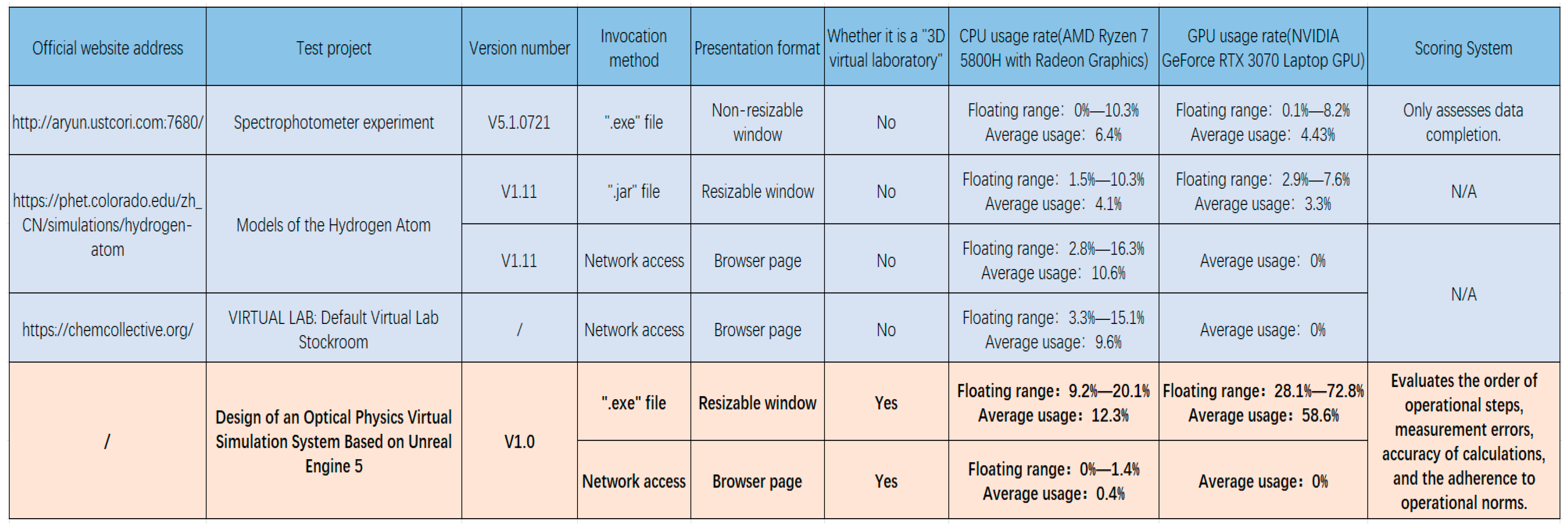
Lower performance requirements. As this system is a 3D virtual simulation experiment, the real-time rendering of scene models and lighting effects consumes more system resources compared to 2D experiments. Therefore, the “.exe” program of this system is not included in the performance comparison. It only demonstrates that web-based access using Unreal Engine 5’s pixel streaming technology has lower requirements for computer performance. By delving into the well-known virtual simulation platforms such as phET and Chem Collective, the performance superiority of the system is compared based on CPU usage (AMD Ryzen 7 5800H with Radeon Graphics) and GPU usage (NVIDIA GeForce RTX 3070 Laptop GPU), as shown in Figure 10. The web-based CPU average usage of Unreal Engine 5 is only 0.4%, reducing the CPU usage by 90.24% to 96.23% compared to the other three platforms, with an average saving of 94.76%. Additionally, the GPU usage for network access in this system is 0%, saving GPU resources compared to non-network-access simulations.

(5)

Comprehensive scoring system. None of the platforms in references [8,11,12], or the three virtual simulation platforms in Figure 10, have a complete scoring system. A scoring system is beneficial in assessing students’ performance in experiments and providing targeted feedback. This system can evaluate students’ understanding of operational procedures, provide information on measurement accuracy by comparing the measured results with standard values, analyze the calculation process, check the accuracy of calculations, and assess the ability to follow operational norms. It facilitates teaching assistance for educators, enhancing the teaching efficiency.

(6)

Has real-time exception handling. During the experiment with the spectrometer in Figure 10, system crashes occurred without error codes for issue feedback. However, when designing the system using a generic architecture approach, it integrates Unreal Engine 5’s exception monitoring tools to monitor the system’s exceptions in real time (such as Unreal Insights performance analysis and debugging tools, the Crash Reporter crash reporting tool, the Bugsnag exception monitoring tool, and the Custom Logging tool, etc.). When users encounter system crashes or similar situations, the system automatically sends error logs to the database to identify the specific location causing the crash or error.

(7)

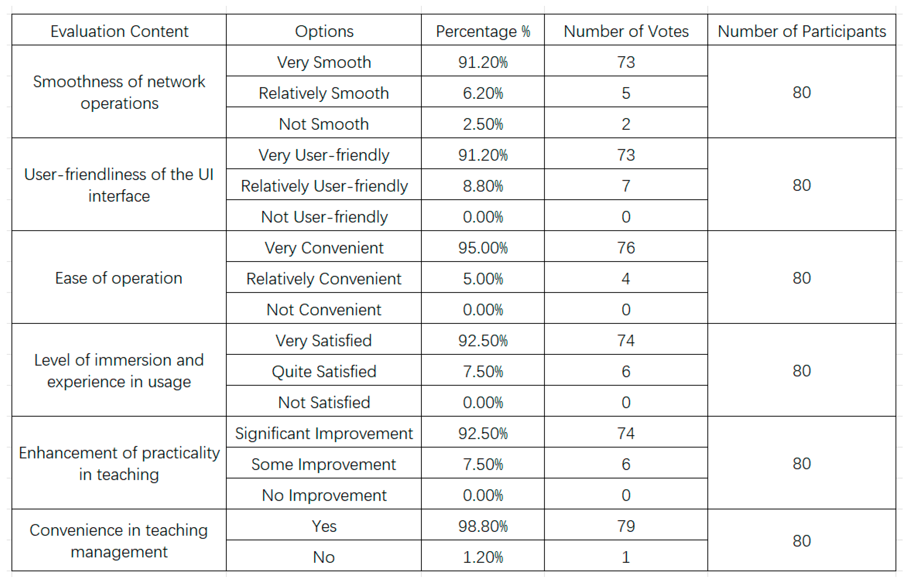
Positive reputation. During the trial phase after the completion of system development, in-depth experiences were provided to professionals and students from various disciplines. A comprehensive survey was conducted, resulting in the collection and analysis of 80 survey reports, as shown in Figure 11. By analyzing the data in the figure, it is evident that each evaluation category received a positive rating exceeding 90%. The system has gained an excellent reputation in real-world environments.

6. Conclusions

The optical physics virtual simulation system designed based on Unreal Engine 5 adopts a generic architecture design approach. This approach enhances the interactivity and realism of virtual simulation experiments, providing a strong sense of immersion. When conducting simulation experiments through network access, it consumes almost no computer resources (as shown in Figure 10, with average CPU usage of 0.4% and GPU usage of 0%, saving approximately 94.76% in average CPU usage compared to the other three platforms). In the future, coherent light sources will be added to simulate more diverse physical phenomena. The Fresnel effect will be incorporated to enhance the authenticity and accuracy of the simulation. Additionally, to address the limitations of a single physics course and improve the breadth and depth of teaching, content from other disciplines, such as chemistry, mathematics, biology, etc., needs to be introduced. This will increase the quantity and quality of the experiments in the simulation system. By complementing virtual simulations with traditional offline physics experiments, the overall effectiveness of physics laboratory teaching will be further improved.

References

1. Huang, J.D. Construction of the Virtual Simulation Experiment Platform for the Physics Experimental Teaching Demonstration Center. Comput. Knowl. Technol. 2019, 15, 261–264+274. [Google Scholar]
2. Wijaya, P.A.; Widodo, A. Muslim Virtual experiment of simple pendulum to improve student’s conceptual understanding. J. Phys. Conf. Ser. 2021, 1806, 012133. [Google Scholar] [CrossRef]
3. Asiksoy, G. Effects of Virtual Lab Experiences on Students’ Achievement and Perceptions of Learning Physics. Int. J. Online Biomed. Eng. 2023, 19, 31. [Google Scholar] [CrossRef]
4. Artun, H.; Durukan, A.; Temur, A. Effects of virtual reality enriched science laboratory activities on pre-service science teachers’ science process skills. Educ. Inf. Technol. 2020, 25, 5477–5498. [Google Scholar] [CrossRef]
5. Brinson, J.R. Learning outcome achievement in non-traditional (virtual and remote) versus traditional (hands-on) laboratories: A review of the empirical research. Comput. Educ. 2015, 87, 218–237. [Google Scholar] [CrossRef]
6. Reeves, S.M.; Crippen, K.J. Virtual laboratories in undergraduate science and engineering courses: A systematic review, 2009–2019. J. Sci. Educ. Technol. 2021, 30, 16–30. [Google Scholar] [CrossRef]
7. Husnaini, S.J.; Chen, S. Effects of guided inquiry virtual and physical laboratories on conceptual understanding, inquiry performance, scientific inquiry self-efficacy, and enjoyment. Phys. Rev. Phys. Educ. Res. 2019, 15, 010119. [Google Scholar] [CrossRef]
8. Niu, H.B.; Li, Y.X.; Liu, H.L.; Wang, X.K. Virtual system of physics experimental instruments based on Unity 3D. Phys. Exp. 2021, 41, 32–37. [Google Scholar]
9. Wang, J.W.; Liang, H.N. Application of virtual simulation technology in spectrometer experimental teaching. Coll. Phys. Exp. 2020, 33, 21–23. [Google Scholar]
10. Liu, X.; Yang, F.R. Research on adjustment of spectrometer based on simulation experimental platform. Inf. Rec. Mater. 2020, 21, 230–231. [Google Scholar]
11. Hou, D.M.; Chen, W.H.; Ma, J.H. Virtual simulation experiment design based on OpenGL. Lab. Res. Explor. 2019, 38, 89–92. [Google Scholar]
12. Chen, Z.X.; Xu, A.J. Design and implementation of spectrometer experiment system based on virtual reality technology. Mod. Comput. 2019, 35, 93–96. [Google Scholar]
13. Ali, N.; Ullah, S.; Khan, D. Interactive Laboratories for Science Education: A Subjective Study and Systematic Literature Review. Multimodal Technol. Interact. 2022, 6, 85. [Google Scholar] [CrossRef]
14. Zhang, M.-H.; Su, C.-Y.; Li, Y.-Y. Factors affecting Chinese university students’ intention to continue using virtual and remote labs. Australas. J. Educ. Technol. 2020, 36, 169–185. [Google Scholar] [CrossRef]
15. Xiao, X.; Liu, X.; Xiao, Z. Construction and Application of Computer Virtual Simulation Teaching Platform for Medical Testing. J. Phys. Conf. Ser. 2021, 1915, 042074. [Google Scholar] [CrossRef]
16. Zhang, Z.; Du, J.; Zhang, W. Application of virtual simulation experiment system in instrumental analysis teaching in colleges. ITM Web Conf. 2022, 45, 01085. [Google Scholar] [CrossRef]
17. Cui, Y.; Lai, Z.; Li, Z.; Su, J. Design and implementation of electronic circuit virtual laboratory based on virtual reality technology. J. Comput. Methods Sci. Eng. 2021, 21, 1125–1144. [Google Scholar] [CrossRef]
18. El-Wajeh, Y.A.; Hatton, P.V.; Lee, N.J. Unreal Engine 5 and immersive surgical training: Translating advances in gaming technology into extended-reality surgical simulation training programmes. Br. J. Surg. 2022, 109, 470–471. [Google Scholar] [CrossRef]
19. Zhang, X.; Fan, Y.; Liu, H.; Zhang, Y.; Sha, Q. Design and Implementation of Autonomous Underwater Vehicle Simulation System Based on MOOS and Unreal Engine. Electronics 2023, 12, 3107. [Google Scholar] [CrossRef]
20. Monji-Azad, S.; Kinz, M.; Hesser, J.; Löw, N. SimTool: A toolset for soft body simulation using Flex and Unreal Engine. Softw. Impacts 2023, 17, 100521. [Google Scholar] [CrossRef]
21. Jiang, C.; Dhamankar, S.; Liu, Z.; Vinod, G.; Shaver, G.; Evans, J.; Puryk, C.; Anderson, E.; DeLaurentis, D. Co-simulation of the Unreal Engine and MATLAB/Simulink for Automated Grain Offoading. IFAC-PapersOnLine 2022, 55, 379–384. [Google Scholar] [CrossRef]
22. Yang, H.; Xia, Z.; Chen, Y.; Zhu, L.; Dai, L.; Xu, R.; Sun, G.; Yu, H.; Xu, W. Research on visual simulation for complex weapon equipment interoperability based on MBSE. Multimed. Tools Appl. 2023, 1–20. [Google Scholar] [CrossRef]
23. Leng, B.; Gao, S.; Xia, T.; Pan, E.; Seidelmann, J.; Wang, H.; Xi, L. Digital twin monitoring and simulation integrated platform for reconfigurable manufacturing systems. Adv. Eng. Inform. 2023, 58, 102141. [Google Scholar] [CrossRef]
24. Hernández-De-Menéndez, M.; Guevara, A.V.; Morales-Menendez, R. Virtual reality laboratories: A review of experiences. Int. J. Interact. Des. Manuf. 2019, 13, 947–966. [Google Scholar] [CrossRef]
25. Jin, F.Z. Two auxiliary methods for measuring grating constant in grating diffraction experiment. Coll. Phys. 2020, 39, 48–52+56. [Google Scholar]
26. Chen, Z.H.; Xu, S.N.; Lv, Z.Y. Derivation of the Wavelength of Diffracted Grating by Geometric Method and Experimental Research. Phys. Eng. 2022, 32, 161–164. [Google Scholar]
27. Alam, A.; Ullah, S.; Ali, N. The Effect of Learning-Based Adaptivity on Students’ Performance in 3D-Virtual Learning Environments. IEEE Access 2017, 6, 3400–3407. [Google Scholar] [CrossRef]
Figure 1. Spectrometer virtual simulation comparison diagram [8,9,10,11,12].
Applsci 14 00955 g001
Figure 2. Schematic diagram of grating diffraction spectrum.
Applsci 14 00955 g002
Figure 3. Overall design diagram of the virtual simulation system.
Applsci 14 00955 g003
Figure 4. Device adjustment process.
Applsci 14 00955 g004
Figure 5. Visual drag-and-drop window layout.
Applsci 14 00955 g005
Figure 6. Graph depicting the relationship between green light diffraction angles and incident angles.
Applsci 14 00955 g006
Figure 7. Innovative experimental setup.
Applsci 14 00955 g007
Figure 8. Web access interface. (a) Web Operation Innovation Experiment. (b) Basic Web Operation Experiment.
Applsci 14 00955 g008
Figure 9. Comparison of virtual simulation effects. (a) Spectrometer instrument based on Unity 3D [8]. (b) Virtual spectrometer instrument structure [9]. (c) Spectrometer adjustment interface [10]. (d) Diffraction experiment based on OpenGL [11]. (e) Spectrometer based on Unity 3D [12]. (f) Spectrometer experiment based on Unreal Engine 5.
Applsci 14 00955 g009aApplsci 14 00955 g009b
Figure 10. Performance and features comparison chart.
Applsci 14 00955 g010
Figure 11. Survey results chart.
Applsci 14 00955 g011