A Population-Based Search Approach to Solve Continuous Distributed Constraint Optimization Problems

Abstract

Distributed Constraint Optimization Problems (DCOPs) are an efficient framework widely used in multi-agent collaborative modeling. The traditional DCOP framework assumes that variables are discrete and constraint utilities are represented in tabular forms. However, the variables are continuous and constraint utilities are in functional forms in many practical applications. To overcome this limitation, researchers have proposed Continuous DCOPs (C-DCOPs), which can model DCOPs with continuous variables. However, most of the existing C-DCOP algorithms rely on gradient information for optimization, which means that they are unable to solve the situation where the utility function is a non-differentiable function. Although the Particle Swarm-Based C-DCOP (PCD) and Particle Swarm with Local Decision-Based C-DCOP (PCD-LD) algorithms can solve the situation with non-differentiable utility functions, they need to implement Breadth First Search (BFS) pseudo-trees for message passing. Unfortunately, employing the BFS pseudo-tree results in expensive computational overheads and agent privacy leakage, as messages are aggregated to the root node of the BFS pseudo-tree. Therefore, this paper aims to propose a fully distributed C-DCOP algorithm to solve the utility function form problem and avoid the disadvantages caused by the BFS pseudo-tree. Inspired by the population-based algorithms, we propose a fully decentralized local search algorithm, named Population-based Local Search Algorithm (PLSA), for solving C-DCOPs with three-fold advantages: (i) PLSA adopts a heuristic method to guide the local search to achieve a fast search for high-quality solutions; (ii) in contrast to the conventional C-DCOP algorithm, PLSA can solve utility functions of any form; and (iii) compared to PCD and PCD-LD, PLSA avoids complex message passing to achieve efficient computation and agent privacy protection. In addition, we implement an extended version of PLSA, named Population-based Global Search Algorithm (PGSA), and empirically show that our algorithms outperform the state-of-the-art C-DCOP algorithms on three types of benchmark problems.

1. Introduction

The Distributed Constraint Optimization Problems (DCOPs) [1,2,3] are a powerful framework for multi-agent modeling. In DCOPs, multiple agents communicate directly or indirectly and coordinate their value assignments to optimize the aggregate constraint utility. DCOPs have been widely applied in practical problems such as meeting scheduling [4,5,6], smart home [7,8], sensor networks [9,10], multi-robot coordination [11,12], and path coordination [13]. Simultaneously, some important improvements and extensions have been proposed for DCOPs, such as the improving advanced methods [14,15,16,17,18], and the extensions of Asymmetric DCOPs [19,20,21,22] and Dynamic DCOPs [23,24].

The DCOP algorithms are simply classified as complete and incomplete algorithms. The complete algorithms aim to provide a global optimum solution, but the computational and memory overheads are expensive, such as Synchronous Branch-and-Bound (SyncBB) [25], Asynchronous Distributed OPTimization (ADOPT) [2], Distributed Pseudo-tree Optimization Procedure (DPOP) [3,26], and Pseudo-trees-Forward Bounding (PT-FB) [27]. Conversely, the incomplete algorithms obtain an approximate solution by reducing computational and memory overheads, such as Distributed Stochastic Algorithm (DSA) [28], Max-Sum (MS) [9,16], Maximum Gain Message (MGM) [29], ACO_DCOP [30], and LSGA [31].

Although the DCOP framework plays an important role in applications of discrete variables (e.g., action sets of machines in the smart home), they make less sense in applications of continuous variables (e.g., positions of robots in the mobile network). Therefore, Stranders et al. [32] proposed the Continuous DCOP (C-DCOP) framework to extend DCOPs whose variables are continuous and the constraint utilities are functional forms. The C-DOCP algorithms include Continuous MS (CMS) [32], Hybrid CMS (HCMS) [33], Bayesian DPOP (B-DPOP) [34], Particle Swarm Based Continuous DCOP (PCD) [35], Exact Continuous DPOP (EC-DCOP) [36] and extensions (Approximate Continuous DPOP (AC-DPOP), Clustered AC-DPOP (CAC-DPOP), Continuous DSA (C-DSA)), Continuous Cooperative Constraint Approximation (C-CoCoA) [37], and Particle Swarm with Local Decision Based Continuous DCOP (PCD-LD) [38].

Firstly, CMS and HCMS extend discrete MS, where CMS approximates utility functions to piecewise linear functions and HCMS introduces a continuous nonlinear optimization method. However, they are both limited by the forms of utility functions. Secondly, B-DPOP combines the Bayesian optimization with DPOP, but it does not guarantee an intermediate solution quality before convergence. Further, EC-DPOP provides the global optimum solution. AC-DPOP and CAC-DPOP provide approximate solutions and reduce communication overheads by limiting the size of messages. Nevertheless, they both incur exponential memory and computational overheads. Then, PCD introduces Particle Swarm Optimization (PSO) in C-DCOPs to reduce the computational and memory overhead. PCD-LD extends PCD to balance solution quality with memory overhead. Finally, C-CoCoA and C-DSA provide two low-cost methods to solve C-DCOPs, but none of the two algorithms have anytime properties.

Based on the above analysis, we propose two population-based approaches by using basic mathematical operators such as addition and multiplication only to solve C-DCOPs, Population-based Local Search Algorithm (PLSA), and the extension, Population-based Global Search Algorithm (PGSA). The proposed PLSA and PGSA can solve problems with any form of utility functions and outperform gradient-based methods in terms of computational and memory overhead [35].

In the previous paper [39], the idea of population-based local search is applied to centralized optimization problems and exhibits excellent performance. Specifically, the algorithm (i) uses some elite solutions and useful information to guide local search; and (ii) systematically updates the population. In this paper, we customize a population-based local search approach for C-DCOPs, which is more suitable for distributed optimization. Our motivations and contributions to PLSA can be summarized as follows:

• Motivation: The pseudo-tree is a communication structure commonly used in C-DCOP algorithms. The root agent can be aware of the aggregate utility according to the utility passing between all agents. We have two worries: (i) the root agent requires more computational and memory overhead. (ii) The privacy violation during utility passing, even if the privacy violation is minor [40].
  Contribution: Therefore, we use the graph structure in PLSA. The agent only passes its value assignments (instead of utilities received from other neighbors) to neighbors and optimizes the sum of local utilities through the neighbors’ value assignments. An important benefit is that each agent can guarantee equal overhead and privacy.
• Motivation: In distributed optimization, since none of the agents are aware of the quality of the aggregate utilities, the quality of aggregate utility fluctuates with the changes in value assignments. However, the sum of local utilities affects aggregate utility, so we consider that local stability promotes global stability to a certain extent.
  Contribution: Hence, we propose a STATE mechanism for each agent to control the changes in value assignments. Specifically, each agent changes its state (updates or holds values) based on historical values, which can make the current agent terminate the update early and keep local stability.
• Motivation: Falling into the local optimum is always an awkward problem in approximate optimization algorithms, which limits the exploration ability of the algorithm. Similarly, PLSA also faces the problem of falling into the local optimum as an approximate optimization algorithm.
  Contribution: With a simple idea, we introduce a classical mutation operator to jump out of the local optimum. The agent resets each value with probability to a random value from its domain.

PGSA is an extension of PLSA, which considers introducing Breadth First Search (BFS) pseudo-tree technology to guarantee its anytime property while extending local search to global search. Extensive comparative experiments on three randomly generated benchmark problems show that PGSA can improve the solution quality of PLSA, and our algorithms are superior to the state-of-the-art C-DCOP algorithms in terms of solution quality.

The remainder of this paper is organized as follows. Firstly, we introduce the background of the problem, the distributed population, and the BFS pseudo-tree in Section 2. In Section 3, we present the details of our algorithms. Section 4 presents the theoretical analysis. Then, Section 5 exhibits the comparative experiments of our algorithms and the state-of-the-art C-DCOP algorithms. Finally, we give the conclusion and future avenues of research in Section 6.

2. Background

In this section, we firstly introduce the DCOP and C-DCOP framework, which are the necessary background to this paper. Then, we describe the distributed population method, which is the basis of our algorithms. Finally, we present the relevant definitions of the BFS pseudo-tree.

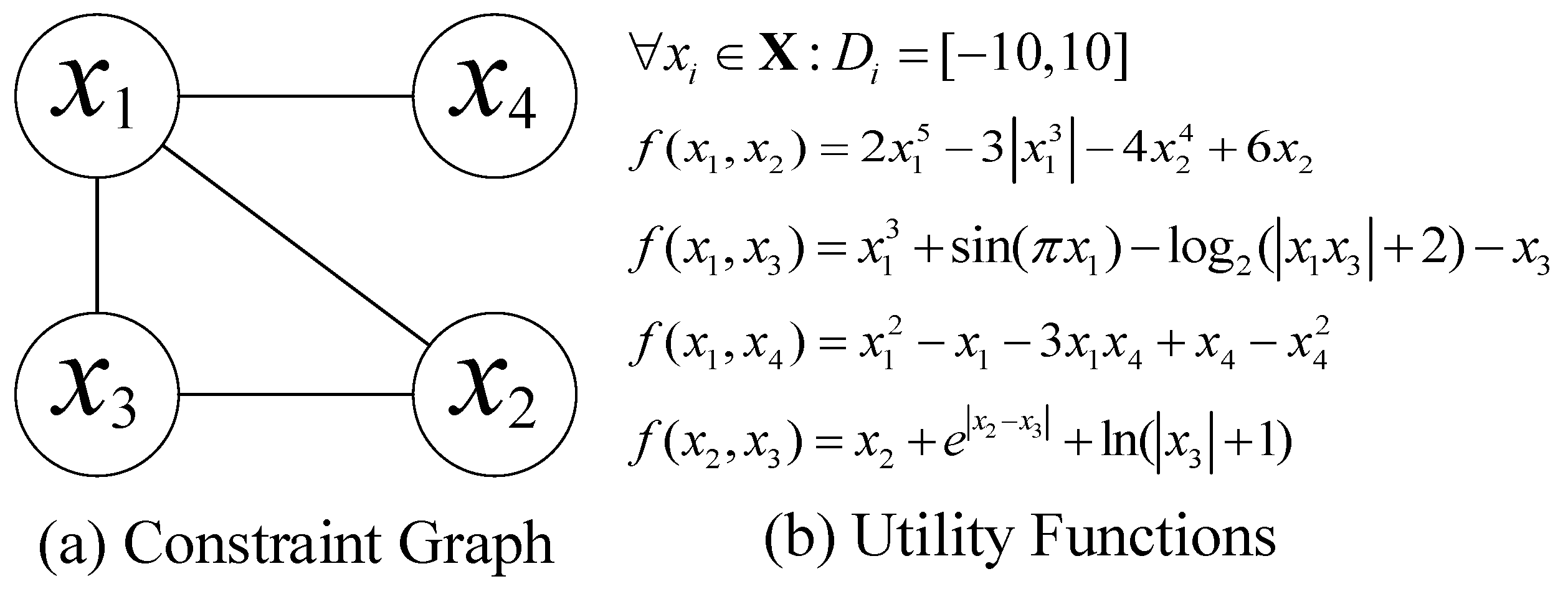
2.1. Distributed Constraint Optimization Problems

A Distributed Constraint Optimization Problem (DCOP) can be defined as a tuple $\langle \mathbf{A},\mathbf{X},\mathbf{D},$$\mathbf{F},\alpha \rangle$, where

• $\mathbf{A}=\{a_1,a_2,\dots ,a_n\}$ is a set of agents; an agent can control one or more variables.
• $\mathbf{X}=\{x_1,x_2,\dots ,x_m\}$ is a set of discrete variables; each variable $x_j$ is controlled by one of the agents $a_i\in \mathbf{A}$.
• $\mathbf{D}=\{D_1,D_2,\dots ,D_m\}$ is a set of discrete domains; each variable $x_i\in \mathbf{X}$ takes value from the domain $D_i\in \mathbf{D}$.
• $\mathbf{F}=\{f_1,f_2,\dots ,f_l\}$ is a set of utility functions; each $f_i\in \mathbf{F}:D_{i_1},D_{i_2},\dots ,D_{i_k}\to \mathbb{R}$ specifies the utility function assigned to each combination of $x_{i_1},x_{i_2},\dots ,x_{i_k}$, where the arity of the utility function $f_i$ is k. We consider that all utility functions are binary (thus $f_{ij}\in \mathbf{F}:D_i\times D_j\to \mathbb{R}$) in this paper.
• $\alpha :$ is a variable-to-agent mapping function that associates each variable $x_j\in \mathbf{X}$ to one agent $a_i\in \mathbf{A}$. In this paper, we assume one agent controls only one variable ($n=m$, thus the terms “agent” and “variable” could be used interchangeably).

The solution of a DCOP is an assignment combination $X^{*}$ to all variables that minimize (we are going to consider the minimization in this paper) the aggregate utility, as shown in Equation (1).

$$\begin{array}{c}\hfill X^{*}=\underset{d_i\in D_i,d_j\in D_j}{\arg \min }{\sum }_{f_{ij}\in \mathbf{F}}{f}_{ij}(x_i=d_i,x_j=d_j)\end{array}$$

(1)

2.2. Continuous Distributed Constraint Optimization Problems

Similarly, a Continuous DCOP (C-DCOP) is a tuple $\langle \mathbf{A},\mathbf{X},\mathbf{D},\mathbf{F},\alpha \rangle$, where $\mathbf{A}$, $\mathbf{F}$, and $\alpha$ are the same as DCOP. The set of variables $\mathbf{X}$ and the set of domains $\mathbf{D}$ are defined as follows:

• $\mathbf{X}=\{x_1,x_2,\dots ,x_m\}$ is the set of continuous variables and each variable $x_j$ is controlled by one of the agents $a_i\in \mathbf{A}$.
• $\mathbf{D}=\{D_1,D_2,\dots ,D_m\}$ is the set of continuous domains and each continuous variable $x_i\in \mathbf{X}$ takes any value from the domain $D_i=[L{B}_i,U{B}_i]$, where $LB$ and $UB$ represent the lower and upper bounds of the domain, respectively.

The goal of a C-DCOP is the same as Equation (1). Figure 1 shows a simple example of a C-DCOP, where Figure 1a shows a constraint graph with four variables, and each edge represents a utility function defined in Figure 1b. The domain $D_i$ of variable $x_i$ is $[-10,10]$.

2.3. Distributed Population

The distributed population is an extension of the traditional population, which has become a basic technology in the population-based algorithm for DCOPs and C-DCOPs [30,31,35,38] in recent years. The distributed population is held collaboratively by all agents.

Table 1. The distributed population.

	Agent ${\mathit{x}}_1$	Agent ${\mathit{x}}_2$	…	Agent ${\mathit{x}}_{\mathit{n}}$
solution 1	$S_1.x_1$	$S_1.x_2$	…	$S_1.x_n$
solution 2	$S_2.x_1$	$S_2.x_2$	…	$S_2.x_n$
…	…	…	…	…
solution k	$S_k.x_1$	$S_k.x_2$	…	$S_k.x_n$
…	…	…	…	…
solution K	$S_K.x_1$	$S_K.x_2$	…	$S_K.x_n$

shows a distributed population of n agents and K solutions, the agent $x_i$ holds one dimension of each solution, and multiple solutions are composed of a population, denoted as S.

One of the solutions, solution $k=\{S_k.x_1,S_k.x_2,\dots ,S_k.x_n\}$, represents an assignment combination of all agents. For solution k, we use $S_k.x_i$ to denote the variable held by agent $x_i$, and we define that $S_k\left(U_i\right)$ represents the sum of local utilities of agent $x_i$, calculated by Equation (2).

$$\begin{array}{c}\hfill S_k\left(U_i\right)={\sum }_{j\in N_i}{f}_{ij}(S_k.x_i,S_k.x_j)\end{array}$$

(2)

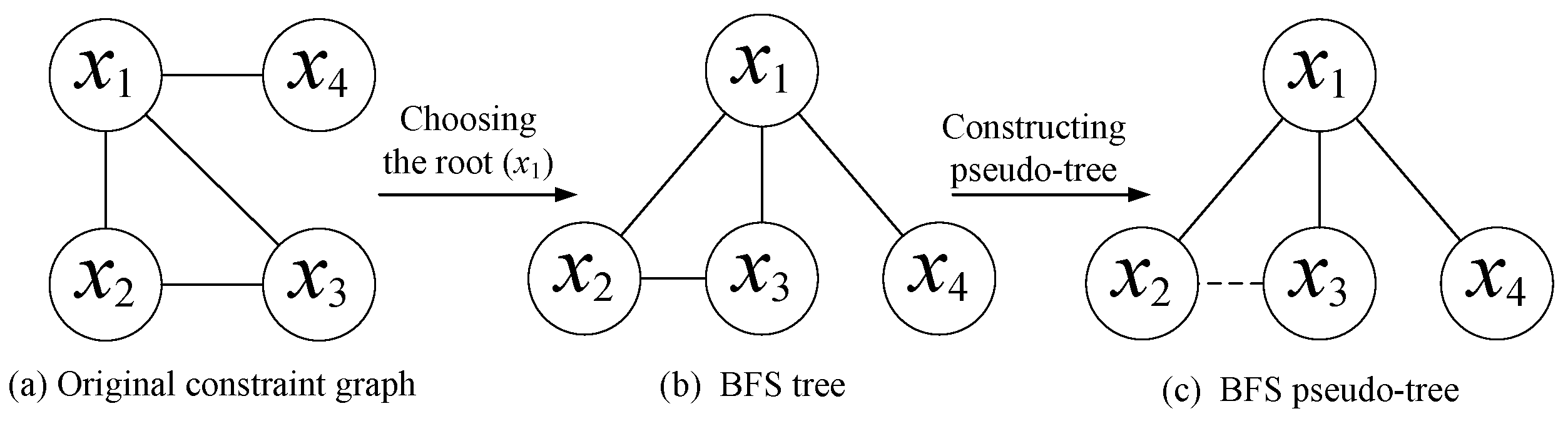
2.4. Breadth First Search Pseudo-tree

The Breadth First Search (BFS) pseudo-tree is a commonly used communication structure for DCOPs and C-DCOPs [3,26,27,35,36,38]. The characteristics of the BFS pseudo-tree are multi-branch parallel computing, short communication path, and time. We briefly present the relevant definitions of the BFS pseudo-tree, and the details can be found in reference [41].

Figure 2 shows an example of a BFS pseudo-tree using the constraint graph in Figure 1a. Some definitions of the BFS pseudo-tree are given as follows:

• $E(x_i,x_j)$—the tree edge, which connects $x_i$ and $x_j$ (e.g., $E(x_1,x_2)$ is a tree edge in Figure 2).
• $CE(x_i,x_j)$—the cross-edge, which directly connects node $x_i$ and $x_j$ in two different branches (e.g., $CE(x_2,x_3)$ is a cross-edge in Figure 2).
• $P_i$— the parent of node $x_i$, the single higher node directly connecting $x_i$ through a tree edge (e.g., $P_2=x_1$ in Figure 2).
• $C_i$— the set of children of node $x_i$, the lower nodes directly connecting $x_i$ through tree edges (e.g., $C_1=\{x_2,x_3,x_4\}$ in Figure 2).
• $N_i$—the set of neighbors of node $x_i$, the neighboring nodes that directly connect $x_i$ (e.g., $N_3=\{x_1,x_2\}$ in Figure 2).
• $P{N}_i$—the set of pseudo-neighbors of node $x_i$, the neighboring nodes that directly connect $x_i$ through cross-edge edges (e.g., $P{N}_3=\left\{x_2\right\}$ in Figure 2).

The BFS pseudo-tree is used for utility aggregation in distributed algorithms, each node $x_i$ sends the sum of local utilities to the root node according to the parent node $P_i$. Finally, the root node is aware of the aggregate utility.

3. Our Algorithms

In this section, we describe the details of the Population-based Local Search Algorithm (PLSA), which is a fully decentralized C-DCOP algorithm. In addition, we introduce a Population-based Global Search Algorithm (PGSA) based on PLSA.

3.1. Population-Based Local Search Algorithm

The PLSA consists of three phases: Initialization, Decision, and Update phases; the details of the algorithm can be found in Algorithm 1.

The Initialization phase: Firstly, PLSA initializes some parameters and constructs a distributed population. Specifically, K represents the number of solutions, and T is the termination parameter, which is the threshold of the agent state change. $\lambda$ and $P_m$ represent the learning rate and mutation probability, respectively. Secondly, each agent sets the $\delta$ to 0 and the STATE to “ACTIVE”. The $\delta$ records the change of the best value, and the STATE determines whether the value assignments are updated. In addition, each agent initializes the current dimension of each solution to a random value from its domain. Finally, the agent $x_i$ sends the values $S.x_i$ to neighbors $N_i$ (Algorithm 1: Lines 3–10).

The Decision phase: When receiving the value assignments $S.x_j$ sent by the neighbor $N_{i_j}\in N_i$, the agent $x_i$ calculates the sum of local utilities $U_i$ of each solution according to Equation (2) (Algorithm 1: Lines 12–14). In addition, agent $x_i$ calculates the index of the best value $best1$ and outputs $S_{best1}.x_i$, which is the value that minimizes the sum of local utilities (Algorithm 1: Lines 15–16).

The Update phase: This phase mainly includes state updates and value updates. On the one hand, the agent $x_i$ compares the best value of the current and the previous iteration. The $\delta$ is increased by one if the two values are equal, otherwise, the $\delta$ is set to zero. Further, if $\delta >T$, the agent $x_i$ changes the STATE to “Hold” (Algorithm 1: Lines 21–26), where t represents the number of iterations. On the other hand, the agent $x_i$ updates each value $S_k.x_i$ and sends it to neighbors $N_i$. Specifically, if the current STATE is “Hold”, each value is updated to $S_{best1}.x_i$. Otherwise, the agent $x_i$ generates a random number $r_m\in [0,1]$ and $S_k.x_i$ is assigned a random value from its domain if $r_m<P_m$. On the contrary, $S_k.x_i$ is updated from a linear combination of the two best and worst values, as shown in Equation (3) (Algorithm 1: Lines 28–35).

Algorithm 1: Population-based Local Search Algorithm

In general, the best solution has good exploitation ability, but it may fall into a local optimum and reduce the exploration ability. Conversely, the worst solution has better exploration ability. Therefore, we consider the weighted combination in Equation (3), such that each solution learns the exploration and exploitation from other solutions, where $S_{best2}.x_i$ is a value that makes the sum of local utilities the second smallest, and $S_{worst}.x_i$ is a value that maximizes the sum of local utilities.

$$\begin{array}{c}\hfill S_k.x_i=(1-\lambda )\ast S_k.x_i+\lambda \ast (S_{best1}.x_i+S_{best2}.x_i-S_{worst}.x_i)\end{array}$$

(3)

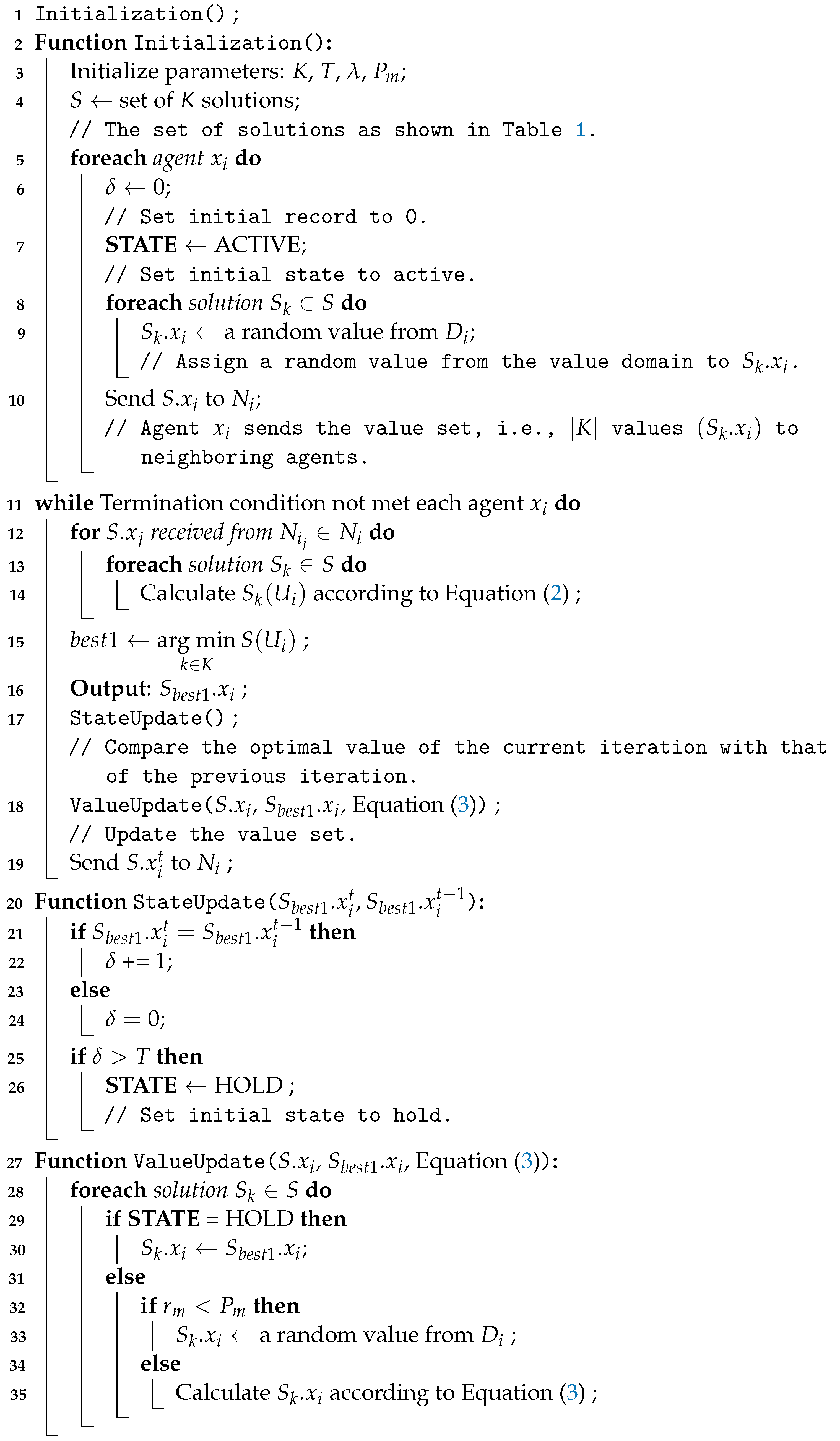
3.2. Population-Based Global Search Algorithm

Similar to PLSA, PGSA, represented by Algorithm 2, includes three phases: Initialization, Decision, and Update phases.

The Initialization phase: PGSA starts the $initialization\left(\right)$ after constructing a BFS pseudo-tree and assigning $\Gamma$ to $+\infty$, where $\Gamma$ records the best aggregate utility. In addition, each agent $x_i$ sets the $Gbes{t}_i$ to complete the assignment combination of the best aggregate utility (Algorithm 2: Lines 1–4).

The Decision phase: Similarly, the agent calculates the sum of local utilities with neighbors (Algorithm 2: Lines 6–8). However, the agent $x_i$ in PSGA sends the sum of local utilities to the parent agent $P_i$. Each agent except the root agent does the same thing; the agent $x_i$ waits to receive the sum of local utilities of children agents $C_i$ and adds it to its sum of the local utilities $S\left(U_i\right)$ (Algorithm 2: Lines 9–15). Since the agents of each layer pass the sum of local utilities up the pseudo-tree and the utility function represented by each edge is calculated twice by the corresponding two agents, the root agent calculates the aggregate utility of each solution by Equation (4). The root agent compares the minimum aggregate utility with $\Gamma$. If the minimum aggregate utility is less than $\Gamma$, the update is assigned the “Assign” and sent by the root agent to neighbors (Algorithm 2: Lines 27–37).

$$\begin{array}{c}\hfill \mathbf{U}=\frac{1}{2}{\sum }_{x_i\in X}{U}_i\end{array}$$

(4)

The Update phase: The agent $x_i$ updates $Gbes{t}_i$ according to the value of update (Algorithm 2: Lines 20–21). In addition, each agent updates its state and value assignments. As an extension of PLSA, we consider the same weighted combination method to update the solution, but we extend the local search to the global search, as shown in Equation (5), where the $S_0$ and $S_{K-1}$ are the solutions with minimum and maximum aggregate utility, respectively. And the $S_1$ is the solution with the second smallest aggregate utility.

$$\begin{array}{c}\hfill S_k.x_i=(1-\lambda )\ast S_k.x_i+\lambda \ast (S_0.x_i+S_1.x_i-S_{K-1}.x_i)\end{array}$$

(5)

Algorithm 2: Population-based Global Search Algorithm

4. Theoretical Analysis

In this section, we prove the anytime property of PGSA and provide some theoretical properties of PLSA and PGSA in terms of communication, computation, and memory. We assume that the graph structure is a binary constraint graph $G=(N,E)$, the number of nodes is $\left|A\right|$, and the number of edges of the constraint graph is $\left|F\right|$. Since the agent calculates the sum of local utilities (Algorithm 1: Line 14 and Algorithm 2: Line 8) or adds the sum of utilities of children agents (Algorithm 2: Line 14) in the decision phase, and the agent updates its value assignments in the update phase (Algorithm 1: Line 18 and Algorithm 2: Line 23), we define one iteration as the entire process of the decision and update phase.

Theorem 1.

PGSA is an anytime algorithm.

Proof. 

In PGSA, the root agent tracks the aggregate utility through a pseudo-tree. We assume that the $\Gamma$ and the aggregate utility $\mathbf{U}$ at the m iterations are ${\Gamma }^m$ and ${\mathbf{U}}^m$, respectively. According to Algorithm 2, Line 32-33, the ${\Gamma }^m\le {\mathbf{U}}^m$. Only the root agent finds the aggregate utility ${\mathbf{U}}^{m+\Delta }$ at the $m+\Delta (\Delta >0)$ iterations and ${\mathbf{U}}^{m+\Delta }<{\Gamma }^m\le {\mathbf{U}}^m$, ${\Gamma }^{m+\Delta }$ is assigned the value of ${\mathbf{U}}^{m+\Delta }$, the ${\Gamma }^{m+\Delta }<{\Gamma }^m$. Otherwise, ${\Gamma }^m$ maintains the best aggregate utility so far. In other words, ${\Gamma }^{m+\Delta }\le {\Gamma }^m$ and the aggregate utility decreases monotonically as the number of iterations increases. Therefore, the PGSA is an anytime algorithm. □

Theorem 2.

The total number of messages of PLSA and PGSA with t iterations are $2t\left|F\right|$ and $4t\left|F\right|$, respectively.

Proof. 

In one iteration of PLSA, for every constraint $f_{ij}(x_i,x_j)$, the agent $x_i$ sends a message to $x_j$ to share value assignments and vice versa. So there are two messages per edge, and thus the number of messages is $2\ast \left|F\right|$, where $\left|F\right|$ is the number of constraints and also the number of edges. Therefore, the total number of messages of PLSA with t iterations is $2t\left|F\right|$. Similarly, the agent $x_i$ in PGSA sends a message to $x_j$ and receives a message from $x_j$. In addition, the agent $x_i$ sends a message (the sum of utilities) to the parent agent (Algorithm 2: Line 15) and Messages to children agents (Algorithm 2: Line 24). Hence, the total number of messages of PGSA with t iterations is $4t\left|F\right|$. □

Theorem 3.

In one iteration, the message sizes of PLSA and PGSA are, respectively, K and $K+1$, where K is the number of solutions.

Proof. 

In PLSA, the agent sends a message containing K values to its neighbors in one iteration. Therefore, the message size of PLSA in one iteration is K, where K is the number of solutions. In PGSA, the agent sends three types of messages: the values assignments, the sum of local utilities, and Messages, whose message sizes are K, K, and $K+1$, respectively. Hence, the message size of PGSA in one iteration is $max\{K,K,K+1\}=K+1$. □

Theorem 4.

In one iteration, the computational overhead of one agent in PLSA and PGSA are, respectively, $K\left(\right|\mathcal{N}|+1)$ and $K\left(\right|\mathcal{N}|+1+|\mathcal{C}\left|\right)$, where K is the number of solutions, $\left|\mathcal{N}\right|$ is the number of neighbors, and $\left|\mathcal{C}\right|$ is the number of children agents in the BFS pseudo-tree. Further, the overall computational overheads of PLSA and PGSA in one iteration are $K\left(2\right|F|+|A\left|\right)$ and $K\left(2\right|F|+2|A|-1)$, respectively.

Proof. 

We define the number of neighbors of one agent is $\left|\mathcal{N}\right|$. In PLSA, each agent calculates the sum of local utilities with its neighbors and updates the value assignments of K solutions. The computational overhead of one agent in one iteration is $K\left(\right|\mathcal{N}|+1)$. Since ${\sum }_{x_i\in X}|{\mathcal{N}}_i|=2\left|F\right|$, therefore, the overall computational overhead of PLSA is ${\sum }_{x_i\in X}K\left(\right|{\mathcal{N}}_i|+1)=K\left(2\right|F|+\left|A\right|)$. Because BFS pseudo-tree is used in PGSA, we define the number of children of one agent as $\left|\mathcal{C}\right|$. In PGSA, one agent not only calculates the sum of local utilities and updates value assignments but also adds the sum of utilities of children agents. Hence, the computational overhead of one agent in one iteration is $K\left(\right|\mathcal{N}|+1+|\mathcal{C}\left|\right)$. Further, each agent has only one parent agent, while the root agent has no parent agent, so ${\sum }_{x_i\in X}|{\mathcal{C}}_i|=\left|A\right|-1$. Finally, the overall computational overhead of PGSA is ${\sum }_{x_i\in X}K\left(\right|{\mathcal{N}}_i|+1+|{\mathcal{C}}_i\left|\right)=K\left(2\right|F|+2|A|-1)$. □

5. Experiment Results

In this section, we first provide the basic experimental configuration. Then, we show the evolution curves of our algorithms (PLSA and PGSA) and competing algorithms (HCMS, PCD, C-CoCoA, and PCD-LD) on three benchmark problems. Finally, we analyze the solution quality of the six algorithms.

5.1. Experimental Configuration

We evaluate our algorithms and competing algorithms on three benchmark problems as follows: (i) Random Graphs: we refer to the Erdös–Rényi model [42] to provide two random graphs, sparse random graphs (edge probability 0.1) and dense random graphs (edge probability 0.6); (ii) Scale-free Networks: we use the Barabási–Albert (BA) [43] model to generate scale-free networks. Its parameters are $(m_1=15,m_2=7)$; and (iii) Small-world Networks: we use the Watts–Strogatz topology model [44] to generate small-world networks. The number of nearest nodes is 6 and the reconnect probability is 0.5.

We set the number of agents from 50 to 100 for three benchmark problems, and the quantity interval was 10. Although PLSA and PGSA can use any form of utility functions (refer to Figure 1), we followed reference [36,38] and used the utility function in the form of $a{x}^2+bx+cxy+dy+e{y}^2+f$ to fairly present the comparison results, where $a,b,c,d,e$, and f are random numbers in the range $[-5,5]$. In addition, we set the domains of all variables to $[-50,50]$ and the number of iterations to 500. For each experimental configuration, we independently ran each algorithm 30 times and took the average as the experimental result. The experiments were carried out on a computer equipped with Intel(R) Core(TM) i5-10500 CPU, 3.10 GHz processor, and 8 GB RAM.

We considered three important parameters of PLSA, $\lambda , T, and P_m$, and refer to reference [38] to set $P_m=0.01$. For the parameters $(\lambda ,T)$, we discretize $\lambda$ into 0.01–0.9 and T into 50–100 to find a combination with the best solution quality on dense random graphs ($\left|A\right|=100$). Figure 3 shows the relative quality of solutions with different $\lambda$ and T, where we normalize the solution quality by max-min normalization to present the difference. Specifically, the relative quality is $\left(\right|Q|-|Q_{max}\left|\right)/\left(\right|Q_{min}|-|Q_{max}\left|\right)$, where Q is the solution quality, $Q_{max}$ and $Q_{min}$ are the maximum and minimum solution quality, respectively. It is obvious from Figure 3 that the best combination ($\lambda ,T$) is $(0.9,100)$. In addition, we set K to 1000. The parameter configuration of the competing algorithms can refer to HCMS [36], PCD [35], C-CoCoA [37], and PCD-LD [38]. It is worth mentioning that we record the best solution found on the empirical evaluation for each algorithm.

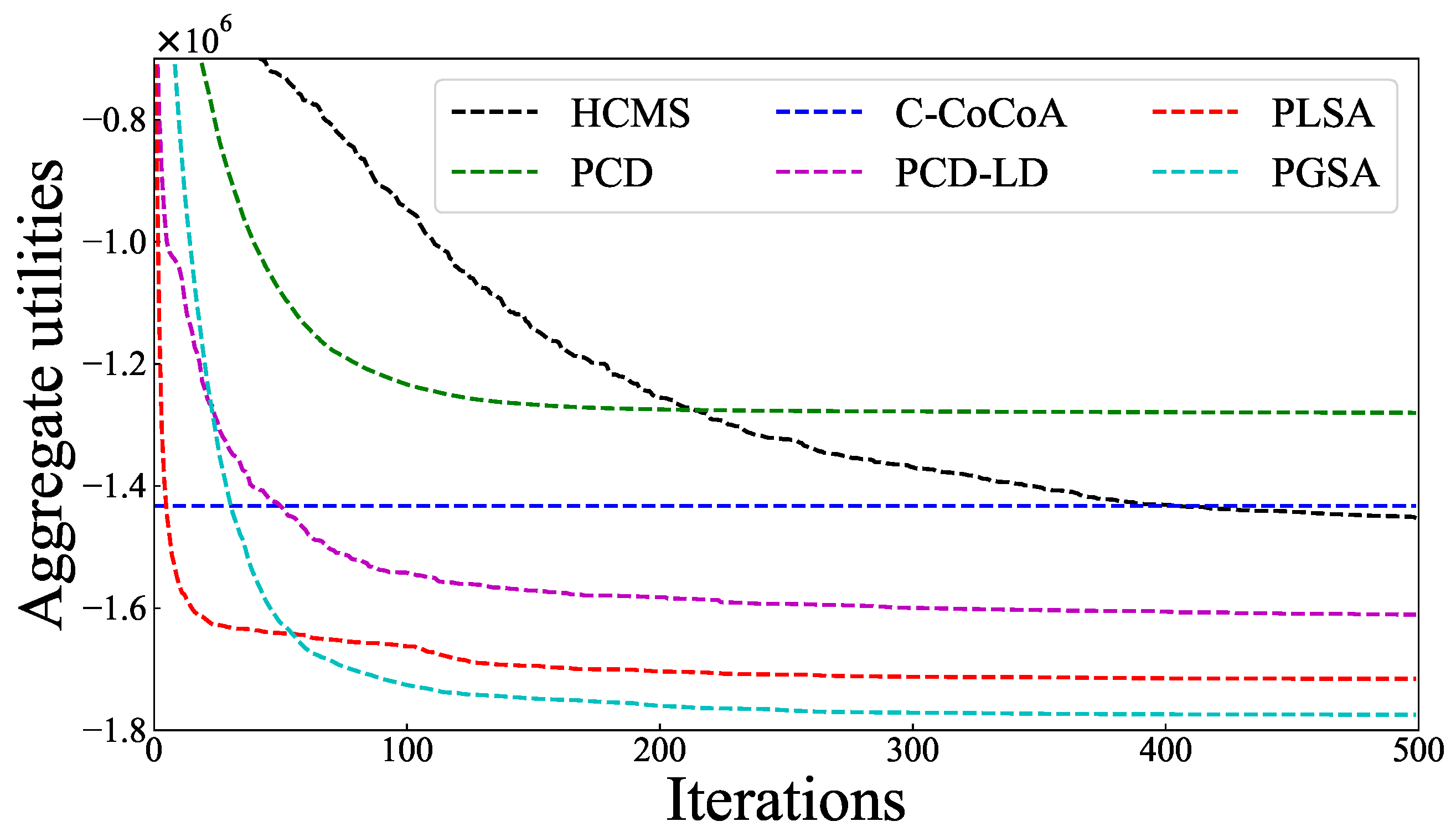
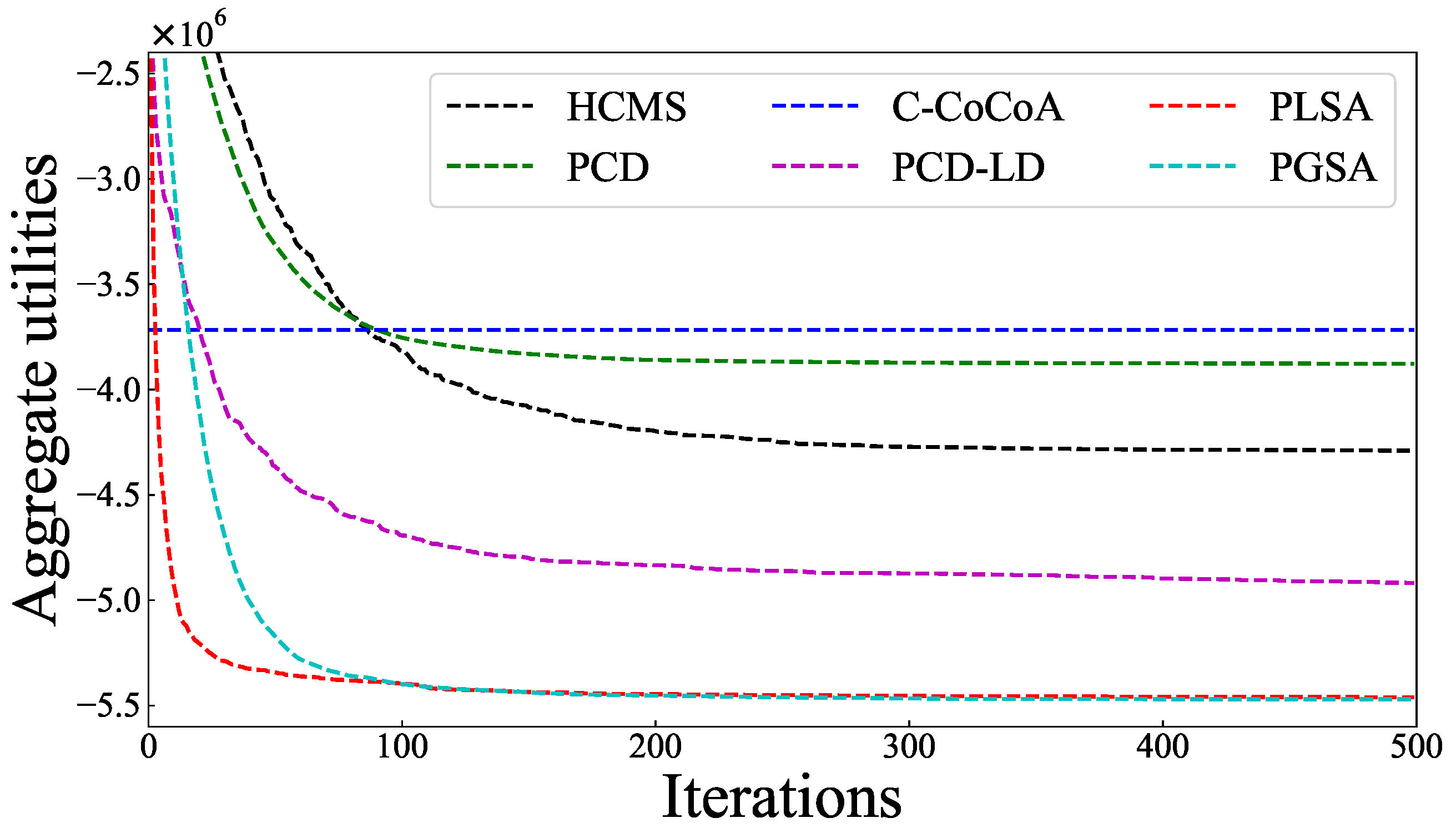
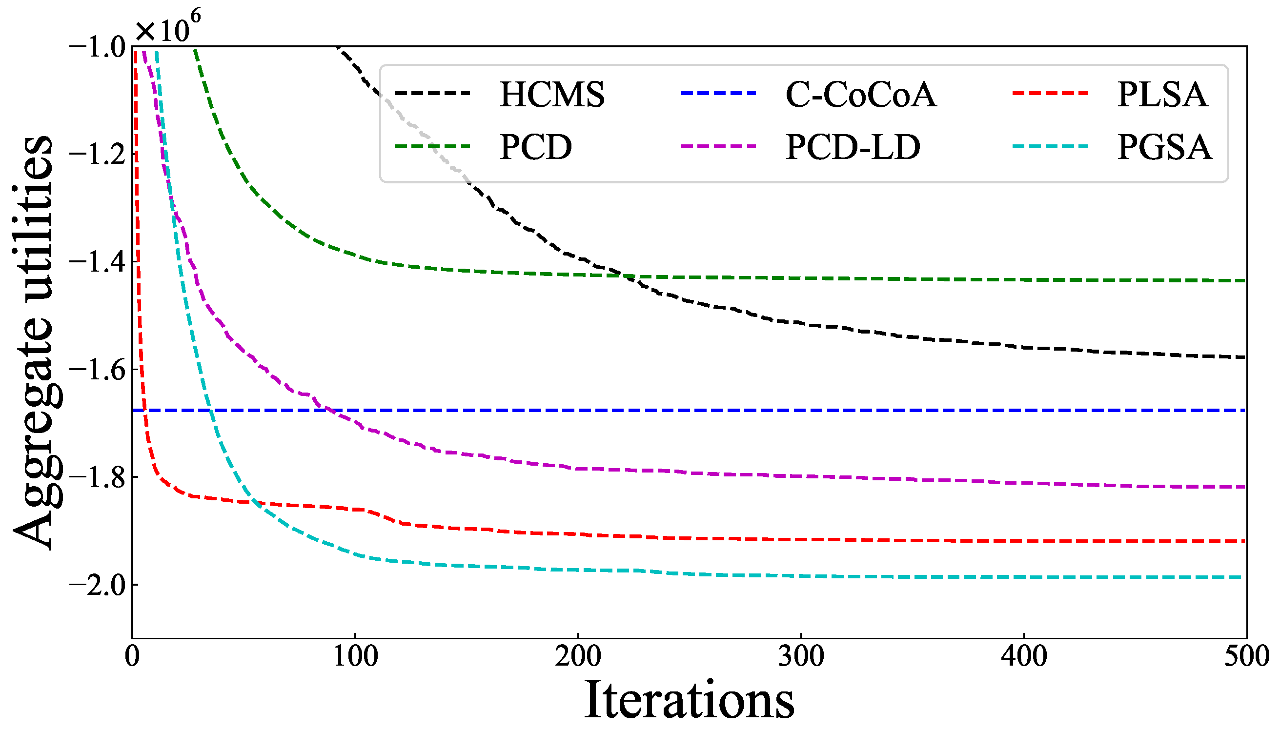
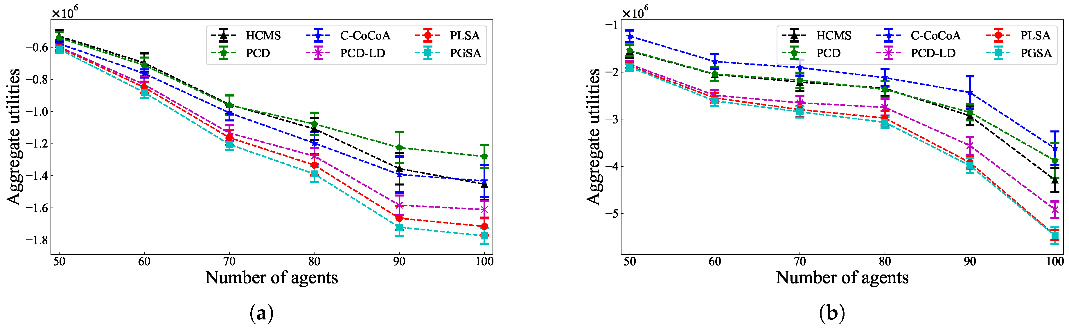
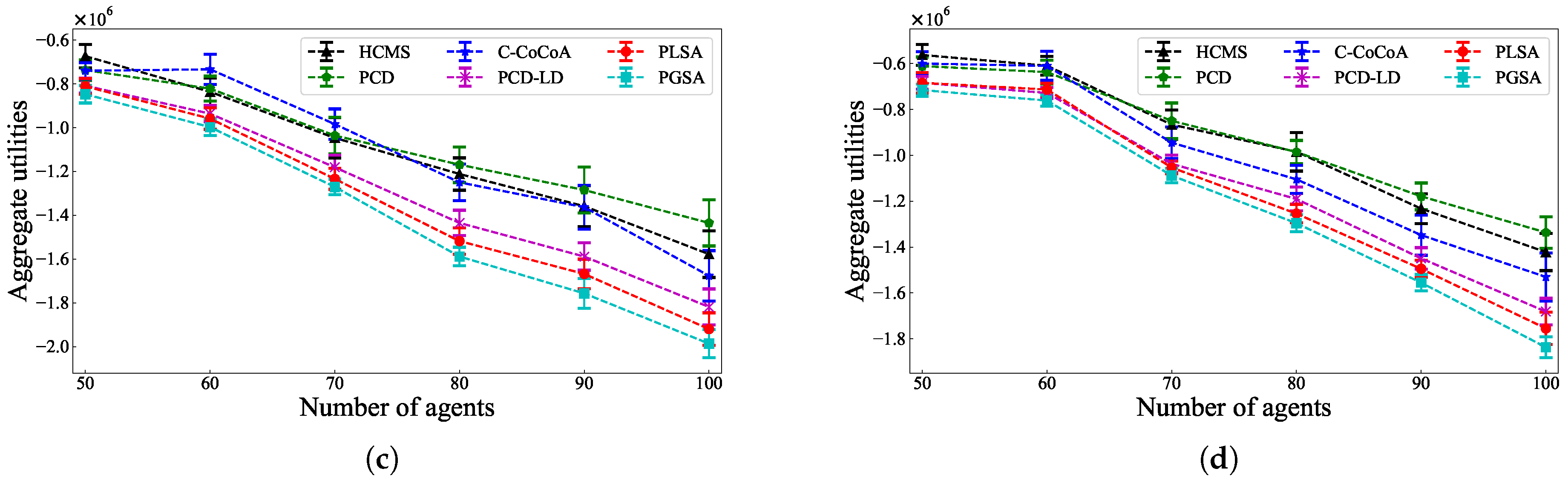
5.2. Comparison of Solution Quality

We present the evolution of the solution quality of our algorithms and competing algorithms with the increasing number of iterations on three benchmark problems with 100 agents. Since C-CoCoA is a non-iterative algorithm, we plot the solution quality of C-CoCoA as a straight line and focus only on its solution quality.

Figure 4 and Figure 5 show the evolution of solution quality of the six algorithms on sparse and dense random graphs, respectively. It can be seen from Figure 4 that PLSA obtains a high-quality solution through a few iterations, and the solution quality of PLSA is significantly superior to competing algorithms. Compared to the local search, there is a better exploration ability in the global search for the solution space. Although PLSA has excellent exploitation for solutions in early iterations, PGSA can explore a higher quality solution by global search. In Figure 5, PLSA and PGSA show the same performance as in sparse random graphs, but a significant difference is that the final solution quality of PLSA and PGSA is similar. The reason for this is that, as the number of neighboring agents on dense random graphs increases, the agents perform local searches over larger search spaces to obtain better solutions. It is worth noting that the solution quality of C-CoCoA is better than that of PCD and similar to HCMS on sparse random graphs, but in dense configurations, its solution quality is worse than PCD and HCMS. The reason for this is that C-CoCoA uses a semi-greedy local search method, for which it is easier to find high-quality solutions on simple graph structures than complex ones. In summary, PLSA and PGSA outperform competing algorithms on both sparse and dense random graphs.

Figure 6 and Figure 7 present the solution quality of PLSA and PGSA against competing algorithms on scale-free and small-world networks, respectively. We can clearly observe that the solution quality of PCD is better than that of HCMS before about 240 iterations. However, as the number of iterations increases, the solution quality of HCMS is superior to that of PCD, and the solution quality of PCD-LD is better than C-CoCoA. Since the global search in PGSA focuses on the exploration of solution space, and the exploitation ability of PGSA for solutions is not as good as that of PCD-LD, PCD-LD initially performs slightly better than PGSA in the early iterations. As the number of iterations increases, the solution quality of PGSA is superior to competing algorithms. In the end, our algorithms significantly outperform competing algorithms on these two benchmark problems.

Further, we evaluate the solution quality of our algorithms and competing algorithms on each benchmark problem with different numbers of agents, and the results are presented in Figure 8. We can see that the solution quality of our algorithm significantly outperforms HCMS, PCD, and C-CoCoA on three benchmark problems with each number of agents. Compared to PCD-LD, the superiority of PLSA and PGSA increases obviously in terms of solution quality as the number of agents increases.

5.3. Statistical Analysis

To clarify the superiority of our algorithms from a statistical perspective, we use the Wilcoxon signed rank test for statistical analysis on each benchmark problem with 100 agents, and the results are shown in

Table 2. Wilcoxon signed rank test results of solution quality over 30 independent runs of our algorithms and competing algorithms with the significance level ${\alpha }_{sl}=0.05$, where $R^{+}$ and $w^{-}$, respectively, represent the times and rank sum. The solution quality of our algorithms is better than that of competing algorithms; $R^{-}$ and $w^{-}$ mean the opposite, respectively. In addition, p represents the p-value.

Type	Ours	HCMS			PCD			C-CoCoA			PCD-LD
		${\mathit{R}}^{+}/{\mathit{R}}^{-}$	${\mathit{w}}^{+}/{\mathit{w}}^{-}$	p	${\mathit{R}}^{+}/{\mathit{R}}^{-}$	${\mathit{w}}^{+}/{\mathit{w}}^{-}$	p	${\mathit{R}}^{+}/{\mathit{R}}^{-}$	${\mathit{w}}^{+}/{\mathit{w}}^{-}$	p	${\mathit{R}}^{+}/{\mathit{R}}^{-}$	${\mathit{w}}^{+}/{\mathit{w}}^{-}$	p
Sparse	PLSA	30/0	465/0	0.000	30/0	465/0	0.000	30/0	465/0	0.000	28/2	441/24	0.000
	PGSA	30/0	465/0	0.000	30/0	465/0	0.000	30/0	465/0	0.000	29/1	464/1	0.000
Dense	PLSA	30/0	465/0	0.000	30/0	465/0	0.000	30/0	465/0	0.000	30/0	465/0	0.000
	PGSA	30/0	465/0	0.000	30/0	465/0	0.000	30/0	465/0	0.000	30/0	465/0	0.000
Scale-free	PLSA	30/0	465/0	0.000	30/0	465/0	0.000	28/2	462/3	0.000	25/5	414/51	0.000
	PGSA	30/0	465/0	0.000	30/0	465/0	0.000	30/0	465/0	0.000	29/1	464/1	0.000
Small-world	PLSA	30/0	465/0	0.000	30/0	465/0	0.000	29/1	463/2	0.000	22/8	375/90	0.003
	PGSA	30/0	465/0	0.000	30/0	465/0	0.000	30/0	465/0	0.000	30/0	465/0	0.000

. It can be clearly seen that our algorithms significantly outperform competing algorithms on three benchmark problems.

Table 3. The average improvement rate (rounded to two decimals) of PLSA and PGSA compared to the competing algorithms on three benchmark problems with different numbers of agents, where $\sigma$ represents the standard deviation of the improvement rates.

Graph Type	Our Algorithms	HCMS ($\mathit{\sigma }$)	PCD ($\mathit{\sigma }$)	C-CcCoA ($\mathit{\sigma }$)	PCD-LD ($\mathit{\sigma }$)
Sparse random graphs	PLSA	19.68% (±3.17%)	24.24% (±8.53%)	13.61% (±5.40%)	3.55% (±2.00%)
	PGSA	23.68% (±4.06%)	28.41% (±9.25%)	17.42% (±6.08%)	7.01% (±2.58%)
Dense random graphs	PLSA	26.57% (±3.97%)	29.83% (±6.94%)	49.03% (±6.66%)	6.52% (±3.56%)
	PGSA	28.70% (±4.26%)	31.97% (±6.43%)	51.50% (±6.13%)	8.30% (±3.49%)
Scale-free networks	PLSA	20.43% (±3.42%)	23.19% (±8.47%)	20.65% (±6.90%)	3.93% (±1.94%)
	PGSA	25.44% (±4.12%)	28.31% (±9.02%)	25.65% (±7.15%)	8.23% (±2.14%)
Small-world networks	PLSA	20.03% (±3.08%)	22.18% (±7.57%)	13.57% (±1.99%)	2.06% (±2.54%)
	PGSA	27.45% (±2.31%)	27.57% (±7.16%)	18.65% (±3.28%)	6.59% (±1.98%)

lists the average improvement rates of PLSA and PGSA compared to HCMS, PCD, C-CoCoA, and PCD-LD on three benchmark problems. In addition, we calculate the standard deviation of the improvement rates under the same problem and show it next to the average improvement rate, denoted as $\sigma$. We can observe that the average improvement rates of our algorithms compared to HCMS and PCD are stable and more than 20%. Compared to C-CoCoA, the average improvement rates of PLSA and PGSA are not stable on different benchmark problems, since C-CoCoA has a better performance on simple graph structures. The average improvement rates of PLSA and PGSA are stable compared to PCD-LD, which are, on average, about 4% and 7%, respectively.

6. Conclusions and Future Work

The C-DCOP framework extends the DCOP framework to solve applications with continuous variables. Addressing the limitations of the utility function and computational overheads for the existing C-DCOP algorithms, we designed a fully decentralized algorithm (PLSA) and a global search anytime algorithm (PGSA). In PLSA, each agent only exchanges value assignments with neighbors to avoid privacy leakage. In PGSA, agents pass utility through pseudo-tree to achieve global search and guarantee anytime property. In summary, there is less computational and memory overhead in PLSA, and it can obtain high-quality solutions faster. PGSA guarantees the anytime property and achieves higher quality solutions, but it requires more computational and memory overhead for utility passing. Extensive evaluations on three benchmark problems demonstrate that our algorithms outperform the state-of-the-art C-DCOP algorithms in terms of the runtime and solution quality. However, there are two limitations: (i) PLSA adopts a stochastic strategy to escape from the local optimum, which may lead to instability in the solution; and (ii) PGSA converges slowly in the early period since it performs the global search. Therefore, the future research avenues can be summarized as follows: (i) we plan to combine some other heuristic methods to improve the quality of and maintain stability in PLSA’s solution; and (ii) we will try to modify the search strategy of PGSA to improve its convergence speed.

7. Discussions

In recent years, the C-DCOPs have been widely studied as an extension framework of DCOPs. As a basic problem framework, there are many other extension frameworks of DCOPs that have become research hot-spots, such as Asymmetric DCOPs (ADCOPs) [45], Multi-objective DCOPs (MO-DCOPs) [46], Dynamic DCOPs (D-DCOPs) [47], Probabilistic DCOPs (P-DCOPs) [48], etc. Accordingly, many algorithms have been proposed for solving different DCOPs-based frameworks. Specifically, in contrast to DCOPs, the utility generated by one agent in ADCOPs from a utility function may differ from the utility generated by another agent from the same utility function. Therefore, the authors of reference [45] extend DSA and proposes Asymmetric Coordinated Local Search (ACLS) to solve ADCOPs, which changes its value with a certain probability to escape from local minimums. The authors of reference [49] solve ADCOPs by employing the PT-ISABB algorithm, which adopts customized inference algorithms to provide strict upper and lower bounds and adopts a complete tree-based search to guarantee optimal performance. In [50], AsymDPOP is proposed to solve the privacy exposure problem in ADCOPs. For MO-DCOPs, the authors of reference [51] propose Multi-objective Synchronous Branch and Bound (MO-SBB) to solve it; the agents in MO-SBB extend the Current Partial Assignment (CPA) with their own assignments with the current utility vector. Once a non-dominated solution is found, it is broadcasted to all agents and the solution is added to the global bounding list. In addition, the authors of reference [52] adopt the concept of non-dominated bounded vectors and retain only non-dominated vectors to solve MO-DCOPs. Then, the D-DCOPs are proposed to cope with environmental evolution over time. The authors of reference [53] introduces an inference-based approach and employ the Hybrid Algorithm for Reconstructing Pseudo-trees (HARP) to solve D-DCOPs, which reuses previous DCOP information to accelerate the search for solutions. In addition [54], the authors employ a reinforcement learning approach to solve D-DCOPs. Finally, P-DCOPs are proposed to cope with environments with stochastic behavior, i.e., there are unexpected events that affect the agent’s behavior. The authors of reference [55] propose a sampling and inference-based algorithm called E-DPOP to solve P-DCOPs, which employs a collaborative sampling strategy to influence the random variables controlled by the agent, and a leading agent merges the set of variables after that. On the other hand, the authors of reference [56] propose the Distributed Neighbor Exchange Algorithm (DNEA) algorithm to solve P-DCOPs. Specifically, each agent in DNEA computes the utility vector with the neighboring agents and sends it to the neighbors. After that, the neighboring agent computes the best value for each of its variables and assigns those values to it probabilistically. The neighboring agent finally sends the assigned values to all its neighbors.

In summary, DCOPs are a widely used basic framework for multi-intelligent systems. With the development of practical applications, different versions of DCOPs-based frameworks have been proposed, and they have made great contributions for solving multi-intelligent system problems. Compared to C-DCOPs, the variables in the above DCOPs-based frameworks are discrete, thus incorporating continuous variables into different extended frameworks is an interesting area of study. Note that the Dynamic Continuous DCOPs (DC-DCOPs), which combine D-DCOPs and C-DCOPs, are provided in reference [47]. This means that exploring different DCOPs versions for continuous variables would be a worthy development.

References

1. Fioretto, F.; Pontelli, E.; Yeoh, W. Distributed constraint optimization problems and applications: A survey. J. Artif. Intell. Res. 2018, 61, 623–698. [Google Scholar] [CrossRef]
2. Modi, P.; Shen, W.M.; Tambe, M.; Yokoo, M. ADOPT: Asynchronous distributed constraint optimization with quality guarantees. Artif. Intell. 2005, 161, 149–180. [Google Scholar] [CrossRef]
3. Petcu, A.; Faltings, B. A scalable method for multiagent constraint optimization. In Proceedings of the 19th International Joint Conference on Artificial Intelligence, Edinburgh, Scotland, 28–30 July 2005; pp. 266–271. [Google Scholar]
4. Hoang, K.D.; Fioretto, F.; Hou, P.; Yokoo, M.; Yeoh, W.; Zivan, R. Proactive dynamic distributed constraint optimization. In Proceedings of the 15th International Conference on Autonomous Agents and Multiagent Systems, Singapore, 9–13 May 2016; pp. 597–605. [Google Scholar]
5. Maheswaran, R.T.; Tambe, M.; Bowring, E.; Pearce, J.P.; Varakantham, P. Taking DCOP to the real world: Efficient complete solutions for distributed multi-event scheduling. In Proceedings of the 3rd International Conference on Autonomous Agents and Multiagent Systems, New York, NY, USA, 19–23 July 2004; pp. 310–317. [Google Scholar]
6. Enembreck, F.; Barthès, J.A. Distributed constraint optimization with MULBS: A case study on collaborative meeting scheduling. J. Netw. Comput. 2012, 35, 164–175. [Google Scholar] [CrossRef]
7. Fioretto, F.; Yeoh, W.; Pontelli, E. A multiagent system approach to scheduling devices in smart homes. In Proceedings of the 16th International Conference on Autonomous Agents and Multiagent Systems, São Paulo, Brazil, 8–12 May 2017; pp. 981–989. [Google Scholar]
8. Rust, P.; Picard, G.; Ramparany, F. Using message-passing DCOP algorithms to solve energy-efficient smart environment configuration problems. In Proceedings of the 25th International Joint Conference on Artificial Intelligence, New York, NY, USA, 9–15 July 2016; pp. 468–474. [Google Scholar]
9. Farinelli, A.; Rogers, A.; Petcu, A.; Jennings, N.R. Decentralised coordination of low-power embedded devices using the max-sum algorithm. In Proceedings of the 7th International Conference on Autonomous Agents and Multiagent Systems, Estoril, Portugal, 12–16 May 2008; pp. 639–646. [Google Scholar]
10. Yeoh, W.; Yokoo, M. Distributed problem solving. AI Mag. 2012, 33, 53–65. [Google Scholar] [CrossRef]
11. Zivan, R.; Yedidsion, H.; Okamoto, S.; Glinton, R.; Sycara, K.P. Distributed constraint optimization for teams of mobile sensing agents. Auton. Agent. Multi. Agent. Syst. 2015, 29, 495–536. [Google Scholar] [CrossRef]
12. Yedidsion, H.; Zivan, R. Applying DCOP_MST to a team of mobile robots with directional sensing abilities. In Proceedings of the 15th International Conference on Autonomous Agents and Multiagent Systems, Singapore, 9–13 May 2016; pp. 1357–1358. [Google Scholar]
13. Picard, G. Trajectory coordination based on distributed constraint optimization techniques in unmanned air traffic management. In Proceedings of the 21st International Conference on Autonomous Agents and Multiagent Systems, Virtual Event, 9–13 May 2022; pp. 1065–1073. [Google Scholar]
14. Chen, Z.; Deng, Y.; Wu, T. An iterative refined max-sum_ad algorithm via single-side value propagation and local search. In Proceedings of the 16th International Conference on Autonomous Agents and Multiagent Systems, São Paulo, Brazil, 8–12 May 2017; pp. 195–202. [Google Scholar]
15. Cohen, L.; Galiki, R.; Zivan, R. Governing convergence of max-sum on DCOPs through damping and splitting. Artif. Intell. 2020, 279, 103212. [Google Scholar] [CrossRef]
16. Khan, M.M.; Tran-Thanh, L.; Jennings, N.R. A generic domain pruning technique for GDL-based DCOP algorithms in cooperative multi-agent systems. In Proceedings of the 17th International Conference on Autonomous Agents and Multiagent Systems, Stockholm, Sweden, 10–15 July 2018; pp. 1595–1603. [Google Scholar]
17. Khan, M.M.; Tran-Thanh, L.; Yeoh, W.; Jennings, N.R. A near-optimal node-to-agent mapping heuristic for GDL-based DCOP algorithms in multi-agent systems. In Proceedings of the 17th International Conference on Autonomous Agents and Multiagent Systems, Stockholm, Sweden, 10–15 July 2018; pp. 1604–1612. [Google Scholar]
18. Zivan, R.; Parash, T.; Cohen, L.; Peled, H.; Okamoto, S. Balancing exploration and exploitation in incomplete min/max-sum inference for distributed constraint optimization. Auton. Agent. Multi. Agent. Syst. 2017, 31, 1165–1207. [Google Scholar] [CrossRef]
19. Deng, Y.; Chen, Z.; Chen, D.; Zhang, W.; Jiang, X. AsymDPOP: Complete inference for asymmetric distributed constraint optimization problems. In Proceedings of the 28th International Joint Conference on Artificial Intelligence, Macao, China, 10–16 August 2019; pp. 223–230. [Google Scholar]
20. Leeuwen, C.J.; Pawelczak, P. CoCoA: A non-iterative approach to a local search (A)DCOP solver. In Proceedings of the 31st AAAI Conference on Artificial Intelligence, 4–9 February 2017; pp. 3944–3950. [Google Scholar] [CrossRef]
21. Zivan, R.; Parash, T.; Cohen-Lavi, L.; Naveh, Y. Applying max-sum to asymmetric distributed constraint optimization problems. Auton. Agent. Multi. Agent. Syst. 2020, 34, 1–29. [Google Scholar] [CrossRef]
22. Deng, Y.; Chen, Z.; Chen, D.; Jiang, X.; Li, Q. PT-ISABB: A hybrid tree-based complete algorithm to solve asymmetric distributed constraint optimization problems. In Proceedings of the 18th International Conference on Autonomous Agents and Multiagent Systems, Montreal QC, Canada, 13–17 May 2019; pp. 1506–1514. [Google Scholar]
23. Hoang, K.D.; Hou, P.; Fioretto, F.; Yeoh, W.; Zivan, R.; Yokoo, M. Infinite-horizon proactive dynamic DCOPs. In Proceedings of the 16th International Conference on Autonomous Agents and Multiagent Systems, São Paulo, Brazil, 8–12 May 2017; pp. 212–220. [Google Scholar]
24. Hoang, K.D.; Fioretto, F.; Hou, P.; Yeoh, W.; Yokoo, M.; Zivan, R. Proactive dynamic distributed constraint optimization problems. J. Artif. Intell. Res. 2022, 74, 179–225. [Google Scholar] [CrossRef]
25. Hirayama, K.; Yokoo, M. Distributed partial constraint satisfaction problem. In Proceedings of the 3rd International Conference on Principles and Practice of Constraint Programming, Linz, Austria, 28–30 October 1997; pp. 222–236. [Google Scholar]
26. Rashik, M.; Rahman, M.M.; Khan, M.M.; Mamun-Or-Rashid, M.; Tran-Thanh, L.; Jennings, N.R. Speeding up distributed pseudo-tree optimization procedures with cross edge consistency to solve DCOPs. Artif. Intell. 2021, 51, 1733–1746. [Google Scholar] [CrossRef]
27. Litov, O.; Meisels, A. Forward bounding on pseudo-trees for DCOPs and ADCOPs. Artif. Intell. 2017, 252, 83–99. [Google Scholar] [CrossRef]
28. Zhang, W.; Wang, G.; Xing, Z.; Wittenburg, L. Distributed stochastic search and distributed breakout: Properties, comparison and applications to constraint optimization problems in sensor networks. Artif. Intell. 2005, 161, 55–87. [Google Scholar] [CrossRef]
29. Maheswaran, R.T.; Pearce, J.P.; Tambe, M. Distributed algorithms for DCOP: A graphical-game-based approach. In Proceedings of the 17th International Conference on Parallel and Distributed Computing Systems, Newport Beach, CA, USA, 9–13 July 2004; pp. 432–439. [Google Scholar]
30. Chen, Z.; Wu, T.; Deng, Y.; Zhang, C. An ant-based algorithm to solve distributed constraint optimization problems. In Proceedings of the 32nd AAAI Conference on Artificial Intelligence, New Orleans, LA, USA, 2–7 February 2018; pp. 4654–4661. [Google Scholar]
31. Chen, Z.; Liu, L.; He, J.; Yu, Z. A genetic algorithm based framework for local search algorithms for distributed constraint optimization problems. Auton. Agent. Multi. Agent. Syst. 2020, 34, 1–31. [Google Scholar] [CrossRef]
32. Stranders, R.; Farinelli, A.; Rogers, A.; Jennings, N.R. Decentralised coordination of continuously valued control parameters using the max-sum algorithm. In Proceedings of the 8th International Conference on Autonomous Agents and Multiagent Systems, Budapest, Hungary, 10–15 May 2009; pp. 601–608. [Google Scholar]
33. Voice, T.; Stranders, R.; Rogers, A.; Jennings, N.R. A hybrid continuous max-sum algorithm for decentralised coordination. In Proceedings of the 19th European Conference on Artificial Intelligence, Lisbon, Portugal, 8–12 August 2010; pp. 61–66. [Google Scholar]
34. Fransman, J.; Sijs, J.; Dol, H.; Theunissen, E.; Schutter, B.D. Bayesian-DPOP for continuous distributed constraint optimization problems. In Proceedings of the 18th International Conference on Autonomous Agents and Multiagent Systems, Montreal, QC, Canada, 13–17 May 2019; pp. 1961–1963. [Google Scholar]
35. Choudhury, M.; Mahmud, S.; Khan, M.M. A particle swarm based algorithm for functional distributed constraint optimization problems. In Proceedings of the 34th AAAI Conference on Artificial Intelligence, New York, NY, USA, 7–12 February 2020; pp. 7111–7118. [Google Scholar]
36. Hoang, K.D.; Yeoh, W.; Yokoo, M.; Rabinovich, Z. New algorithms for continuous distributed constraint optimization problems. In Proceedings of the 19th International Conference on Autonomous Agents and Multiagent Systems, Auckland, New Zealand, 9–13 May 2020; pp. 502–510. [Google Scholar]
37. Sarker, A.; Choudhury, M.; Khan, M.M. A local search based approach to solve continuous DCOPs. In Proceedings of the 20th International Conference on Autonomous Agents and Multiagent Systems, Virtual Event, UK, 3–7 May 2021; pp. 1127–1135. [Google Scholar]
38. Shi, M.; Liao, X.; Chen, Y. A particle swarm with local decision algorithm for functional distributed constraint optimization problems. Intern. J. Pattern. Recognit. Artif. Intell. 2022, 36, 2259025. [Google Scholar] [CrossRef]
39. Abuhamdah, A.; Ayob, M.; Kendall, G.; Sabar, N.R. Population based Local search for university course timetabling problems. Appl. Intell. 2014, 40, 44–53. [Google Scholar] [CrossRef]
40. Zivan, R.; Okamoto, S.; Peled, H. Explorative anytime local search for distributed constraint optimization. Artif. Intell. 2014, 212, 1–26. [Google Scholar] [CrossRef]
41. Chen, Z.; He, Z.; He, C. An improved DPOP algorithm based on breadth first search pseudo-tree for distributed constraint optimization. Artif. Intell. 2017, 47, 607–623. [Google Scholar] [CrossRef]
42. Paul, E.; Rényi, A. On the evolution of random graphs. Publ. Math. Inst. Hung 1960, 5, 17–60. [Google Scholar] [CrossRef]
43. Réka, A.; Albert-László, B. Statistical mechanics of complex networks. Rev. Mod. Phys. 2002, 74, 47. [Google Scholar] [CrossRef]
44. Watts, D.J.; Strogatz, S.H. Collective dynamics of ’small-world’ networks. Nature 1998, 393, 440–442. [Google Scholar] [CrossRef]
45. Grinshpoun, T.; Grubshtein, A.; Zivan, R.; Netzer, A.; Meisels, A. Asymmetric distributed constraint optimization problems. J. Artif. Int. Res. 2013, 47, 613–647. [Google Scholar] [CrossRef]
46. Delle Fave, F.M.; Stranders, R.; Rogers, A.; Jennings, N.R. Bounded decentralised coordination over multiple objectives. In Proceedings of the 10th International Conference on Autonomous Agents and Multiagent Systems, Taipei, Taiwan, 2–6 May 2011; pp. 371–378. [Google Scholar]
47. Hoang, K.D.; Yeoh, W. Dynamic continuous distributed constraint optimization problems. In Proceedings of the 24th International Conference on Principles and Practice of Multiagent Systems, Valencia, Spain, 16–18 November 2022; pp. 475–491. [Google Scholar]
48. Nguyen, D.T.; Yeoh, W.; Lau, H.C. Stochastic dominance in stochastic DCOPs for risk-sensitive applications. In Proceedings of the 11th International Conference on Autonomous Agents and Multiagent Systems, Valencia, Spain, 4–8 June 2012; pp. 257–264. [Google Scholar]
49. Chen, D.; Deng, Y.; Chen, Z.; He, Z.; Zhang, W. A hybrid tree-based algorithm to solve asymmetric distributed constraint optimization problems. Auton. Agent. Multi. Agent. Syst. 2020, 34, 1–42. [Google Scholar] [CrossRef]
50. Chen, D.; Chen, Z.; Deng, Y.; He, Z.; Wang, L. Inference-based complete algorithms for asymmetric distributed constraint optimization problems. Artif. Intell. Rev. 2022, 56, 4491–4534. [Google Scholar] [CrossRef]
51. Medi, A.; Okimoto, T.; Inoue, K. A two-phase complete algorithm for multi-objective distributed constraint optimization. J. Adv. Comput. Intell. Intell. Inform. 2014, 18, 573–580. [Google Scholar] [CrossRef]
52. Matsui, T.; Silaghi, M.; Hirayama, K.; Yokoo, M.; Matsuo, H. Leximin multiple objective optimization for preferences of agents. In Proceedings of the 17th International Conference on Principles and Practice of Multiagent Systems, Gold Coast, QLD, Australia, 1–5 December 2014; pp. 423–438. [Google Scholar]
53. Yeoh, W.; Varakantham, P.; Sun, X.; Koenig, S. Incremental DCOP search algorithms for solving dynamic DCOPs. In Proceedings of the 10th International Conference on Autonomous Agents and Multiagent Systems, Taipei, Taiwan, 2–6 May 2011; pp. 1069–1070. [Google Scholar]
54. Shokoohi, M.; Afsharchi, M.; Shah-Hoseini, H. Dynamic distributed constraint optimization using multi-agent reinforcement learning. Soft Comput. 2022, 26, 360103629. [Google Scholar] [CrossRef]
55. Léauté, T.; Faltings, B. Distributed constraint optimization under stochastic uncertainty. In Proceedings of the 25th AAAI Conference on Artificial Intelligence, San Francisco, CA, USA, 7–11 August 2011; pp. 68–73. [Google Scholar]
56. Atlas, J.; Decker, K. Coordination for uncertain outcomes using distributed neighbor exchange. In Proceedings of the 9th International Conference on Autonomous Agents and Multiagent Systems, Toronto, ON, Canada, 10–14 May 2010; pp. 1047–1054. [Google Scholar]
Figure 1. An example of a C-DCOP.
Applsci 14 01290 g001
Figure 2. A BFS pseudo-tree representation (c) of the C-DCOP depicted in Figure 1a.
Applsci 14 01290 g002
Figure 3. Relative quality of solutions with different λ and T.
Applsci 14 01290 g003
Figure 4. The evolution of solution quality of PLSA and PGSA against the competing algorithms on sparse random graphs.
Applsci 14 01290 g004
Figure 5. The evolution of solution quality of PLSA and PGSA against the competing algorithms on dense random graphs.
Applsci 14 01290 g005
Figure 6. The evolution of solution quality of PLSA and PGSA against the competing algorithms on scale-free networks.
Applsci 14 01290 g006
Figure 7. The evolution of solution quality of PLSA and PGSA against the competing algorithms on small-world networks.
Applsci 14 01290 g007
Figure 8. The solution quality of PLSA and PGSA against the competing algorithms with different numbers of agents. (a) Sparse random graphs. (b) Sense random graphs. (c) Scale-free networks. (d) Small-world networks.
Applsci 14 01290 g008aApplsci 14 01290 g008b