Review

Review of Advances in Active Impulsive Noise Control with Focus on Adaptive Algorithms

School of Microelectronics, Tianjin University, Tianjin 300072, China
*
Author to whom correspondence should be addressed.
Appl. Sci. 2024, 14(3), 1218; https://doi.org/10.3390/app14031218
Submission received: 22 November 2023 / Revised: 26 January 2024 / Accepted: 29 January 2024 / Published: 31 January 2024
(This article belongs to the Special Issue Feature Review Papers in "Acoustics and Vibrations" Section)

Abstract

:
Mitigating low-frequency noise in various industrial applications often involves the use of the filter-x least mean squares (FxLMS) algorithm, which relies on the mean square error criterion. This algorithm has demonstrated effectiveness in reducing noise induced by Gaussian noise within noise control systems. However, the performance of this algorithm experiences significant degradation and does not converge properly in the presence of impulsive noise. Consequently, to uphold the stability of the ANC system, several robust adaptive algorithms tailored to handle shock noise interference have been introduced. This paper systematically organizes and classifies robust adaptive algorithms designed for impulse noise based on algorithmic criteria, offering valuable insights for the research and application of pertinent active impact noise control methods.

1. Introduction

Noise control encompasses both active noise control (ANC) approaches and passive noise control (PNC). Passive noise control primarily involves addressing noise through the manipulation of sound waves and acoustic isolation materials or structural design. This method is highly effective for controlling higher-frequency noise but has several drawbacks when it comes to low-frequency noise control. The characteristics of active noise reduction and passive noise reduction are outlined in Table 1.
Therefore, in recent years, active noise control systems have gained increasing favor due to their compact size and excellent low-frequency noise reduction capabilities. They utilize active noise control algorithms to generate anti-noise signals, which are emitted through acoustic devices such as speakers to eliminate unwanted noise. The two core components of the ANC system are adaptive filters and control algorithms. The coefficients of the adaptive filter are iteratively updated according to the rules of the control algorithm. The filter, guided by the control algorithm, produces a secondary sound source that is equal in magnitude but opposite in phase to the primary noise, resulting in destructive interference to cancel out the primary noise. In 1933, German physicist Paul Lueg first applied active noise cancellation to the treatment of noise at lower frequencies in pipelines, implementing active noise control using the least mean square (LMS) algorithm [1]. In 1981, Burgess introduced the filtered-x least mean square (FxLMS) algorithm to address phase shift in the secondary path. Since then, FxLMS has become a classic algorithm in active control methods [2].
Figure 1 illustrates the block diagram of a feedforward ANC system. Where the reference signal is denoted as x(n) = [x(n), x(n − 1),…, x(nL + 1)]T, P(z) signifies the primary path, and the secondary route is represented by S(z). The adaptive filter is used for obtaining the estimation of the secondary path, denoted as S ~ ( z ) , through offline or online modeling techniques. When the filter length is L, the adaptive filter, denoted as W(z), has a weight vector represented as w(n) = [w0(n), w1(n), …, wL−1(n)]T. The represented output response of the filter is y(n):
y n = w T n x n
The expression for the error signal is as follows:
e n = d n - y f n = d n - y n s n
where s(n) corresponds to the response characteristics of S(z) and * signifies the discrete convolution operator. Represented by y f ( n ) and x f ( n ) , these terms stand for the filtered reference and secondary signal, respectively.
The cost function in the FxLMS algorithm entails the square mean of the error signal, with E[∗] denoting the expectation operator:
J ( n ) = E   [ e 2 ( n ) ]
The FxLMS algorithm employs gradient descent to derive the iterative update equation, which is as follows:
w ( n + 1 ) = w ( n ) μ J ( n ) w ( n ) = w ( n ) + μ e ( n ) x f ( n )
The FxLMS algorithm possesses advantages such as simplicity, ease of implementation, and effective active control, making it particularly efficient in handling noise that follows a Gaussian distribution. However, its noise reduction performance significantly diminishes when dealing with impulse noise.
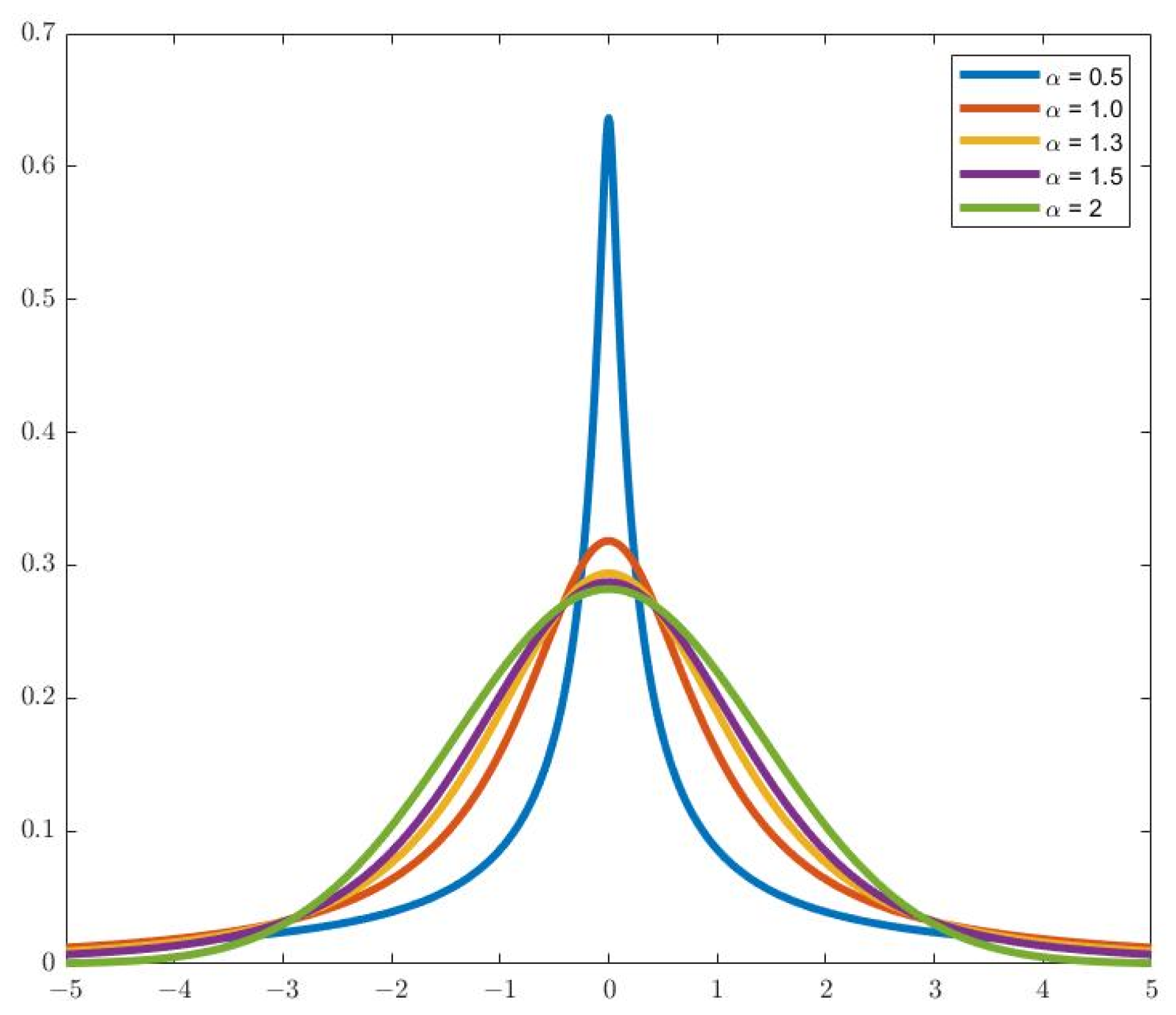
The characteristics of impulse noise can be adequately illustrated using the noise model depicted in Figure 2, which follows a standard SαS distribution. As shown in Figure 2, in the presence of impulse noise, the l2 norm of the error signal exhibits unbounded characteristics. This implies that the e ( n ) , rooted in the MSE, lacks a minimum value, hindering the algorithm from achieving stable convergence.
The SαS distribution is characterized by the following expression for its characteristic function:
V ( t ) = exp j δ t γ | t | α [ 1 + j β s g n ( t ) S ( t , α ) ]
where:
S ( t , α ) =   tan α π 2 α = 1 2 log | y | / π α 1
When α ∈ (0, 2), a decrease in α results in a heavier-tailed probability distribution, increasing the likelihood of outliers in the signal. A smaller α corresponds to a higher degree of noise impulses. In real-life situations, common values for the α of pulse noise range from (1, 2). The graph distinctly illustrates that when α = 0.5, the curve exhibits pronounced peaks and thicker tails, representing an uncommon occurrence in everyday noise. Conversely, when α = 2, the distribution degenerates into a Gaussian distribution. β serves as the symmetry coefficient, where β = 0 indicates a symmetric distribution. The parameter δ signifies the location parameter. γ is the scale parameter.
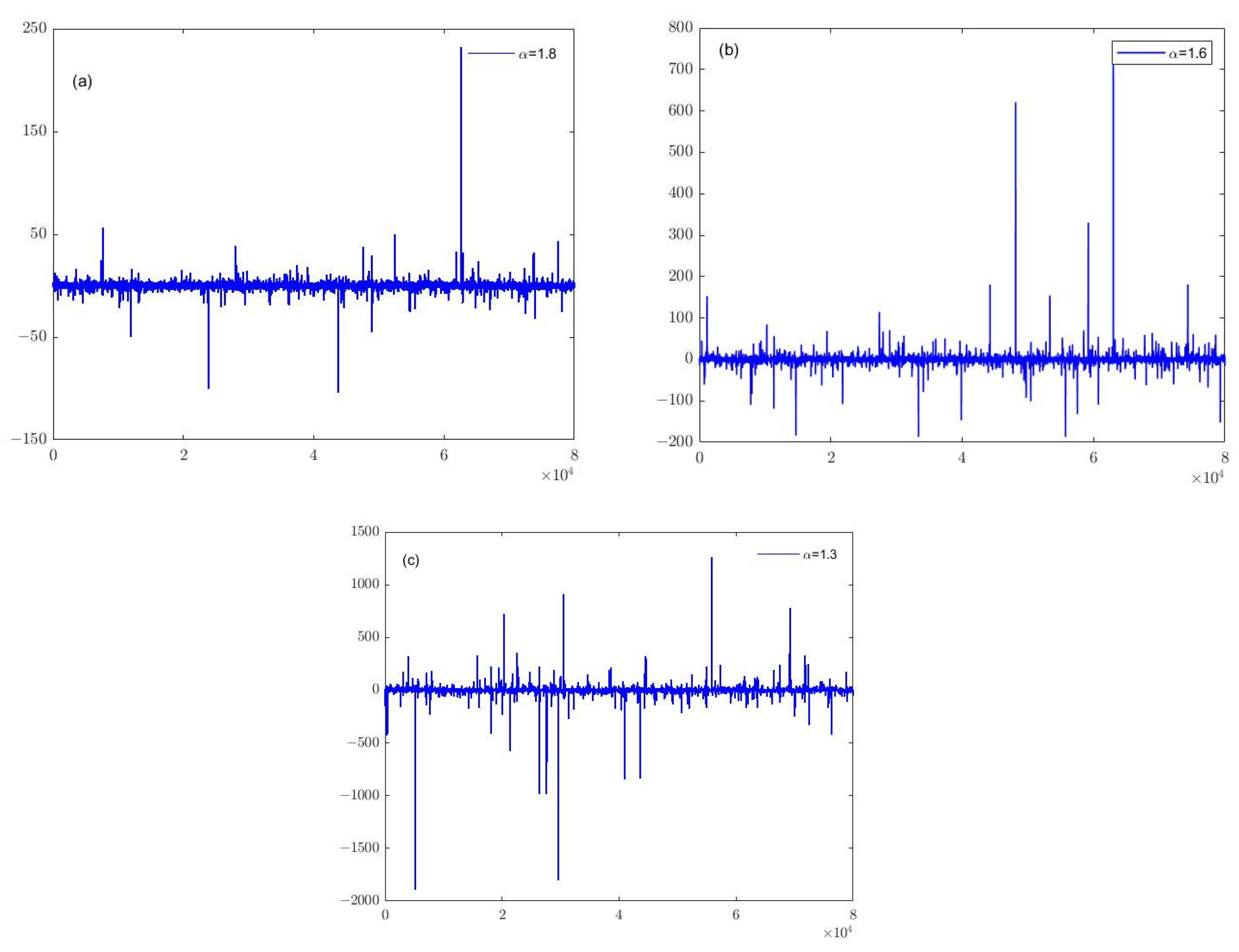
Many everyday situations give rise to impulsive noise. Impulse noise is an unexpected, sharp sound that occurs instantaneously over the course of time. Figure 3 illustrates noise signals with varying intensities under different α values of the α-stable distribution. As observed in Figure 3, a decrease in α leads to increased amplitude and discrete changes in the noise signal, thereby complicating the convergence of algorithms.
Various robust adaptive algorithms, extensively discussed in prior literature, have been developed to improve the stability of ANC systems when confronted with abrupt noise interference. This study systematically organizes and categorizes adaptive algorithms designed explicitly for impulsive noise, classifying them based on their criteria. The aim is to provide a structured summary, offering valuable insights for research and applications in active impulsive noise control.

2. Fractional Lower-Order Power-Based Algorithms

2.1. p-Power Algorithms

From the above, it is evident that when the impulse noise signal follows an α-stable distribution, the l2 norm of the e ( n ) does not exist, but the p power of the e ( n ) is bounded. In lieu of minimizing the variance, as in standard algorithms, Leahy et al. proposed minimizing the existing fractional lower-order moments (p < α) [3]. Here, p represents the order less than the dispersion α. They introduced the filter-x least mean p-power (FxLMP) algorithm, where the cost function aims to minimize the p-power of the e ( n ) . Leahy and colleagues studied the impact of parameter p on the algorithm’s performance and concluded that the closer p is to the characteristic parameter of impulsive noise, the better the algorithm performs. In fact, when setting the parameter p in the FxLMP algorithm to a fixed value, the algorithm degrades into different algorithms such as LMAD, LMAT and LMF [4,5]. Therefore, the FxLMP algorithm can be considered a general algorithm for this type. Subsequently, many researchers improved the FxLMP algorithm based on the study by Leahy. Akhtar and Mitsuhashi, based on the FxLMP algorithm, applied threshold nonlinear transformations to both the reference and error signals. This further improved the robustness of the FxLMP method without increasing computational complexity [6]. However, the stability of the FxLMP algorithm is contingent on the parameter p. The algorithm exhibits better stability when p is less than the characteristic parameter α of impulsive noise. Consequently, it is necessary to estimate the characteristic parameter of impulsive noise in advance when applying the FxLMP method. Bergamasco and Piroddi delved into the dependency of the FxLMP algorithm on the characteristic parameter α of impulsive noise [7]. They proposed a sliding window method for online estimation of the characteristic parameter α. This method circumvents the need for prior knowledge of the characteristic parameter α in p power algorithms but comes at the cost of increased algorithm complexity.
In addition, another drawback of the FxLMP series algorithms is the increased computational complexity and slow convergence speed of ANC systems due to the computation of fractional lower-order powers. To address this, Akhtar and Mitsuhashi, building upon the FxLMP algorithm, introduced two modified algorithms: the modified FxLMP (MFxLMP), which incorporates a threshold method, and the filtered-x modified normalized least mean p power, which utilizes a normalization step size method [8]. The filter-x affine projection (FxAP) algorithm was introduced by S.C. Douglas to address convergence speed in correlated input environments. Subsequently, Akhtar and Nishihara combined the affine projection algorithm with the normalized p power algorithm (FxNLMP) [9]. This integration leveraged the characteristics of the projection algorithm to improve the convergence speed of the algorithm. The results indicate that the algorithm maintains good convergence when transitioning from low-intensity impulse noise (α = 1.7) to high-intensity impulse noise (α = 1.1) and maintains insensitivity to changes in the noise source. In contrast, the FxLMP algorithm becomes unstable. Additionally, the introduction of the projection algorithm results in an increase in computational complexity. Akhtar, building upon the FxLMP, FxNLMP and filtered-x generalized normalized LMP (FxGNLMP) algorithms, proposed the convex-combined step size FxGNLMP algorithm, which enhanced the convergence speed and steady-state performance of active impulsive noise control algorithms [10]. Nevertheless, the convex combination algorithm increased computational complexity due to the parallel computation of two filters. Zheng developed a filter-logarithmic recursive least p-power algorithm, integrating logarithmic moments with p-power norms to enhance the noise reduction performance in the α state of 1.35 [11].
In order to facilitate a more intuitive comparison of various update functions, the filter coefficient update formulas are standardized as follows:
w ( n + 1 ) = w ( n ) + μ φ ( e ( n ) ) x f ( n )
The cost function and filter coefficient update formulas for the fractional lower-order power algorithms are shown in Table 2.
The characteristics of p-power algorithms are summarized. These methods are intricately linked to impulsive noise, influencing the robustness of parameter p. More specifically, the algorithm’s convergence is contingent on the relationship between p and α amidst impulsive noise interference, where effective convergence occurs when p < α. Whether estimating α online or offline, additional steps and computational burden are introduced, contributing to increased algorithm complexity. The computation of the p power of the error signal further amplifies the algorithm’s computational load.
Scholars have sought to enhance the performance of this type of algorithm by employing methods such as normalized step size, filter convex combination and integration with projection algorithms to improve convergence speed and steady-state error. However, these improvement measures cannot prevent the subsequent increase in algorithm complexity.

2.2. Other Algorithms

p-power algorithms need to satisfy p < α to prevent instability in ANC systems. To ensure stability in all situations, the choice of p = 1 has been proposed, leading to the sign algorithm (SA). The SA algorithm, in comparison to the FxLMP algorithm, does not necessitate prior knowledge of the distinctive parameter α of impulsive noise, leading to a reduction in processing demands [12,13]. However, traditional SA trades convergence speed for robustness. To address this, Shao introduced the affine projection sign algorithm, commonly known as APSA, which minimizes the posterior error l1 moment as the optimization goal [14]. By introducing the error sign vector, APSA eliminates the need to invert matrices during weight coefficient updates, significantly reducing algorithmic computational complexity. Simultaneously, the introduction of the error l1 moment enhances the algorithm’s resilience to impulsive noise. The algorithm exhibits excellent resistance to impulse noise interference, enhancing the convergence speed under colored input signals. Yu and Zhao simplified the formula for the proportionality factor in the proportionate affine projection sign algorithm, commonly known as PAPSA, improving the algorithm’s computational efficiency and impulsive noise resilience. The performance of noise reduction in sparse systems is improved [15].
Zhao improved the efficiency and impulsive noise resilience of the proportionate affine projection sign algorithm (PAPSA) by introducing the Gaussian entropy as a substitute for the error l0 moment in the proportionality matrix function along with its approximate formula [16]. Additionally, Li introduced the error sign function and reference signal into the SA step size, allowing for a larger step size during the initial working phase for rapid convergence and a smaller step size with minimal errors to achieve significant steady-state error reduction. The algorithm demonstrates fast convergence under colored input signals, where the smoothing factor parameter satisfies 0 < β < 1 [17]. Wang implemented an enhanced Gaussian kernel formula, replacing the traditional variable step size formula. β represents a smooth factor [18]. Kim expedites the convergence of the APSA algorithm through adaptive step size adjustment [19]. In this context, the parameter δ is typically set to 0, and α is defined as 1-M/5L. This ensures stability when outliers are present. This formula adjusts the step size to be larger when the error is significant, enhancing convergence speed, and smaller when the error is minor, improving steady-state error. Chen and Ni enhanced the convergence speed of the sign algorithm (SA) by introducing a natural logarithmic momentum term related to the absolute value of weight coefficients in the weight coefficient update formula [20]. This algorithm enhances system performance in sparse environments, where ε is a non-zero decimal number. Zong proposed a series of dual sign algorithms (DSA) and introduced compensation terms related to the l1 and l0 moments of weight coefficients in the weight coefficient update formula to accelerate the convergence process in sparse environments [21].
In addition, there are mixed-moment algorithms and continuous p power algorithms. In 1997, Jonathon and Apostolos proposed a method called the mixed norm (MN) algorithm, which forms a new cost function by convexly combining the l2 and l1 norms of the error [22]. Papoulis and Stathaki improved the convergence speed and steady-state performance of the MN algorithm by adapting the fixed mixing parameter in the MN algorithm based on the error and normalizing the step parameter in the weight coefficient update formula [23]. Song and Zhao summarized the general form of the MN algorithm, proposing the filtered-x general mixed norm (FxGMN) algorithm [24]. When p = q = 2 and λ 0 = 0.5 , the algorithm exhibits optimal noise reduction capabilities in pulse environments. They enhanced its convergence speed through convex combination methods and studied the control capability of the FxGMN algorithm for impulsive noise under different parameter combinations. Lu and Zhao employed a continuous logarithmic transformation p-power cost function for active noise control [25]. The algorithm performs well under various secondary path conditions. Hadi, based on the FxLMP algorithm, introduced a continuous mixed p-norm cost formula to improve adaptive algorithms in ANC systems [26]. Feng introduced self-p-normalized algorithms to achieve faster convergence without compromising the stability error characteristics of the system, where ⊙ denotes the Hadamard product and r denotes the intensity of the reference noise [27]. Some algorithm update formulas are shown in Table 3.
In summarizing various algorithms, the sign algorithm stands out for its ability to handle impulsive noise without the need for prior estimation of the characteristic parameter α. However, its drawback lies in a relatively slow convergence speed, necessitating enhancements through techniques like affine projection, variable step size, and momentum. The mixed norm algorithm combines error l1 and l2 moment algorithms, offering a balanced approach, where the former boosts robustness and the latter improves convergence speed. Meanwhile, the continuous p-power algorithm introduces a logarithmic transformation for rapid convergence, albeit at the expense of a higher complexity. Choosing the most suitable algorithm depends on specific application requirements and contextual considerations. When exclusively considering the algorithm’s effectiveness, the FxGMN algorithm is applicable. Due to the property of convex combination, this approach enhances the robustness of the MN algorithm while keeping up with convergence rate. When the primary concern is complexity, the SA algorithm can be used, which is easy to implement, but the algorithm has poor stability in the mixed noise environment with Gaussian noise or in the impact noise with a high intensity. The continuous mixed p-norm algorithm can be used when faster convergence is required.

3. Non-Linear Transformation-Based Algorithms

3.1. Threshold Method

Grounded in the error l2 moment criterion, the FxLMS algorithm experiences significant performance degradation when encountering impulsive noise interference. The simplest and most direct method to mitigate impulsive noise interference is to set thresholds for both the error signal and reference signal. Sun introduced the threshold FxLMS (ThFxLMS) algorithm, which ignores signals with values exceeding a predefined threshold parameter [28]. In this approach, the corresponding filter coefficients remain unchanged, ensuring the stability of the ANC system. However, in specific scenarios, this method may lead to frequent coefficient freezing, resulting in a slower convergence speed. In 2009, Akhtar further improved the algorithm based on the ThFxLMS algorithm [29]. In addition to correcting the reference signal, constraints were applied to the error signal, replacing outliers with critical values. Zhou proposed a method using box plot (BP) sliding windows for online threshold estimation [30]. This method does not require prior knowledge of the impulsive noise characteristic parameter α, and the threshold exhibits time-varying characteristics. Non-linear threshold transformations applied to the reference signal can be utilized not only in FxLMS but also in other algorithms. Saravanan enhanced the algorithm’s control performance against impulsive noise by applying a threshold non-linear transformation to both the error and reference signals and adopting a variable step size approach [31].
In 2007, Thanigai introduced the FxLMM algorithm, utilizing a non-linear transformation of the error signal with the Hampel function. Zhou combining the Huber M-estimation method with the LMS algorithm and presented a simplified FxLMM algorithm [32]. Wu and Qiu utilized the Fair function to transform the error signal, facilitating the setting of thresholds for error signals [33]. Akhter introduced a hyperbolic tangent threshold transformation for both the reference and error signals, replacing the manual threshold-setting approach [34]. Sun improved the FLMM’s performance by substituting a more precise method for estimating the proportion of the distribution in the reference noise with a higher degree of accuracy [35]. The threshold of the algorithm in this classification is obtained through parameter estimation by the formula. Table 4 summarizes the threshold formulas and corresponding weight coefficient update formulas for threshold-based algorithms.
The characteristics of Threshold-Based Algorithms can be seen in Table 4. The fixed threshold method has low computational complexity, but its performance depends on the selection of threshold parameters. Foreknowledge of the distinctive parameter α of abrupt noise is required for the selection of threshold parameters, and adjustments to this parameter are not feasible when noise conditions change. On the other hand, online estimation methods for thresholds have a high computational complexity. Algorithms that implement hyperbolic tangent functions to the input and error signals still require offline estimation of threshold parameters. Robust M estimation algorithms essentially achieve resistance to impulsive noise interference by limiting the error signal.

3.2. Logarithmic Transformation and Trigonometric Transformation

For impulsive noise signals following an α-stable distribution, the signal becomes more Gaussian-like after undergoing a logarithmic transformation. Consequently, Wu introduced the FxlogLMS algorithm, or the filtered-x logarithmic transformation least Mean square algorithm. This algorithm utilizes the error signal after logarithmic transformation as the objective function [36]. This algorithm exhibits stability without the need for prior knowledge of the impulsive noise characteristic parameter α or the estimation of threshold parameters, making it more robust compared to the FxLMP method. However, the FxlogLMS algorithm introduces additional computational complexity due to the logarithmic calculation involved in updating the weight coefficients. Additionally, careful consideration is required for cases where l exceeds the amplitude of the error signal. George and Panda introduced an algorithm that utilizes the logarithmic transformation of the squared error signal as the objective function, specifically designed for impulsive noise elimination [37]. Furthermore, Sayin introduced a convex combination approach, incorporating the logarithmic conversion of the error signal α (α = 1.2) moments [38]. The algorithm corresponding to the l2 moment is referred to as the least mean logarithmic square (LMLS) algorithm, while the l1 moment corresponds to the least logarithmic absolute difference (LLAD) algorithm. Both algorithms exhibit rapid convergence and resilience against impulsive noise interference, although careful parameter selection is essential for their combination. LU introduced a recursive error fractional moment logarithmic transformation algorithm that combines logarithmic transformation with fractional lower-order moment methods [39]. The recursive algorithm enhances the convergence speed of the algorithm but also increases computational complexity. The Lorenz norm, another form of logarithmic transformation, is utilized in algorithms presented by Lochan and Narwaria including the Lorenz norm algorithm based on the error signal, the normalized Lorenz norm algorithm and the momentum Lorenz norm algorithm [40]. These algorithms demonstrate excellent steady-state performance and convergence speeds.
In addition to logarithmic transformations, trigonometric function transformations can enhance the algorithm’s robustness against impulse noise. Mirza utilized the logarithmic hyperbolic cosine transformation of the error signal as the objective function in the filtered-x least cosine hyperbolic (FxLCH) algorithm and proposed the simultaneous use of variable step sizes and threshold nonlinear transformation methods for active elimination of impulse noise [41]. Wang employed the logarithmic hyperbolic cosine transformation of the error signal as the cost function, enhancing the convergence speed of the algorithm through a variable step size form [42]. Patel used the logarithmic hyperbolic cosine transformation of the error signal as the cost function [43]. Since the weight coefficient update formula of this type of algorithm requires calculating the exponential form of the error, the authors proposed two approximation equations, reducing computational complexity. Yu adopted the logarithmic hyperbolic cosine transformation of the error signal as the cost function and improved the algorithm’s convergence speed through an accelerated gradient method [44]. Song utilized the hyperbolic tangent function of the error as the cost function [45]. The parameter β needs adjustment based on the signal impulses and the algorithm. The hyperbolic tangent function adjusts the step size based on the amplitude variation of the error signal in weight coefficient updates. Under impulse noise conditions, the algorithm adapts the stride to bolster system robustness. Conversely, with a decrease in the error signal, the stride is increased to ensure the system convergence rate. Integrating the hyperbolic secant function and the mean difference function, Lu formulated the cost function [46]. This method, with a clever choice of combination parameters, allows the step scaling factor to play a more excellent role. When the system has not encountered impulse noise and the error signal amplitude is large, the step size is not scaled to accelerate convergence. When the error is small, the step size is scaled to enhance steady-state performance. When encountering impulse noise interference, the step size is scaled to strengthen system stability. In Xiao’s proposed algorithm, the random Fourier feature (RFF) technique and CG approach are employed to address the slow convergence issues posed by the generalized Hough transform (GHT) criterion [47].
Zhu proposed an algorithm based on a random Fourier filter to handle impulse noise. The algorithm’s convergence capability is confirmed through numerical simulations under different conditions [48]. Gu introduced the error arctangent as the cost function, presenting the filtered-x arctangent error least mean square (FxatanLMS) algorithm [49]. The study showed outstanding performance of the normalized error arctangent algorithm in handling narrowband, wideband, and impulse noise. Tao proposed a constrained least variance algorithm, demonstrating superior performance in impulse noise environments compared to other algorithms. The lncosh cost function is the natural logarithm of the hyperbolic cosine function, representing a combination of mean square error and mean absolute error criteria [50]. In this paper, setting β to 0.8 achieves the best convergence performance under pulse noise. Krishna Kumar introduced a new robust norm based on the exponential hyperbolic cosine function (EHCF) and developed corresponding adaptive filters based on EHCF [51]. Radhika proposed two adaptive filters based on hyperbolic sine functions that are suitable for impulse noise environments [52]. The study explored learning rate-based stability conditions and steady-state analysis. Additionally, a variable scale parameter format was proposed to eliminate the trade-off between convergence speed and steady-state excess mean squared error. Guan proposed two adaptations based on the hyperbolic secant function (HSF). In the presence of pulse interference, both algorithms exhibit superior performance compared to existing algorithms [53]. Table 5 summarizes the corresponding weight coefficient-updating formulas for algorithms based on logarithmic and trigonometric transformations.
The FxlogLMS algorithm involves logarithmic calculations during the filter weight coefficient updating process, significantly increasing computational complexity. However, other logarithmic transformation weight coefficient updating formulas, excluding FxlogLMS, do not require logarithmic calculations. Logarithmic hyperbolic cosine transformation algorithms essentially limit the amplitude of the error signal. Other types of logarithmic transformations are similar to step size normalization algorithms. These algorithms exhibit slow convergence rates in the presence of Gaussian noise. Three trigonometric functions that are suitable for nonlinear transformation of the error signal are the hyperbolic tangent, hyperbolic secant and arctangent. This type of transformation is a relatively recent introduction as a nonlinear cost function, demonstrating superior performance. However, the weight coefficient updating formulas involve complex trigonometric functions, especially hyperbolic functions, thereby increasing algorithmic complexity.

4. Other Transformation Algorithms

The MCC algorithm, formally known as the maximum correntropy criterion, aims to enhance performance by maximizing the probability of similarity in the local space between two sets of random variables. The core idea of this algorithm is to control the observation range of random variables through the adjustment of kernel width, thereby automatically excluding outliers. The MCC algorithm is essentially based on the mixed second-order norm of the error signal, typically employing a Gaussian kernel function. In the MCC algorithm, increasing the kernel width expands the observation space, making the algorithm gradually approach the FxLMS algorithm. Conversely, decreasing the kernel width narrows the observation space, thereby enhancing the MCC algorithm’s resistance to impulsive noise.
Liu first introduced the concept of correntropy and theoretically analyzed the advantages of the MCC algorithm in handling impulsive noise [54]. The MCC algorithm exhibits l2 moment characteristics when two sets of analyzed signals are relatively similar, presents l1 moment properties when there is a slight difference in signals and shows l0 moment properties when the signal gap is larger. Therefore, it ensures the stability of the active noise control (ANC) system under impulsive noise interference. PRINCIPE utilized the MCC algorithm to identify and eliminate impulsive noise in system recognition under impulsive noise interference [55]. Chen conducted a theoretical analysis, marking the first investigation into the long-term performance of the MCC algorithm and providing insights into its steady-state behavior [56]. Chen proposed the GMCC algorithm, formally known as the generalized maximum correntropy criterion algorithm. They verified the stability of this equation under impulsive noise interference through theoretical derivation and simulation [57]. LU proposed a filtered-x recursive maximum correntropy algorithm with adaptive kernel width updates, demonstrating fast convergence and robustness against impulsive noise [58]. The results indicate that the algorithm exhibits a fast convergence rate in environments with a low pulse intensity (α = 1.7). By integrating the AP algorithm with other methods, Li proposed two novel adaptive approaches for addressing impulsive noise [59]. Zhao presented a multi-convex combination maximum correntropy adaptive algorithm. The synergy of the AP and GMCC algorithms can significantly improve the algorithm’s effectiveness [60]. The algorithm achieves the best convergence performance when the parameter α is set to 2. Wang introduced a transformed kernel width MCC algorithm that operates as a fixed kernel width MCC algorithm when the error is small [61]. The algorithm proposed by Zhou adopts an improved conjugate gradient method to iteratively update filter coefficients, thereby enhancing the algorithm’s performance [62].
Chen introduced the kernel risk-sensitive loss (KRSL) algorithm, demonstrating from theoretical and simulation perspectives that this method achieves a fast convergence, high accuracy and robustness [63]. Zhang combined the minimum kernel risk-sensitive loss criterion with the p-norm method, proposing a new robust adaptive algorithm [64]. Qian introduced the convex combination KRSL algorithm. Similar to the MCC algorithm, the performance of the KRSL algorithm is associated with the kernel width parameter [65]. Information-theoretic learning cost functions have the advantages of strong robustness and not requiring prior estimation of the impulsive noise characteristic parameter α. However, careful selection of the kernel width is necessary for optimal performance of this algorithm.
In addition, Huang combined the maximum skewness line criterion with the FxLMP algorithm, proposing a novel adaptive algorithm [66]. Lei derived a filter-x affine projection algorithm based on the minimum variance distortionless response (MVC) by solving an inequality-constrained problem [67]. This algorithm demonstrates a fast convergence when dealing with active impulsive noise control. Cheng, inspired by convex combination methods, combined the FxLMS algorithm with the FxMVC algorithm, developing the C-FxMVC algorithm using an amplitude constraint approach [68]. Simulation results indicate that the C-FxMVC algorithm performs well in terms of convergence speed and noise reduction. Radhika theoretically analyzed the stability of VersoriaLMS-type algorithms based on the maximum skewness line criterion under Gaussian and non-Gaussian noise conditions [69]. Huang proposed a set of adaptive algorithms belonging to the SigmoidLMS type by embedding conventional cost functions into the sigmoid function [70]. Leveraging the amplitude compression feature of the sigmoid function, this algorithm resists impulsive noise interference. The algorithm introduces a free parameter, aside from the step size, controlling the compression amplitude and influencing convergence speed and steady-state error. The sigmoid function transformation algorithm exhibits some similarity to the hyperbolic tangent transformation.
Omer introduced a robust semi-quadratic criterion (HQC) adaptive filtering algorithm using convex cost functions [71]. The proposed HQC introduces a more efficient performance surface, leading to substantial improvements in dealing with impulsive noise. Krishna proposed a robust algorithm and confirmed through simulation studies that the arctan algorithm family achieves a higher performance compared to standard algorithms [72]. The filter coefficient update formulas for the algorithms are shown in Table 6.
In summary, in practical applications, the first consideration involves determining whether a prior estimate of α is necessary to guide the selection of the appropriate algorithm. Additionally, factors such as the computational complexity and hardware feasibility of the algorithm must be taken into account. The final step is to choose the appropriate algorithm based on the severity of the pulse noise. It is worth noting that in real life, pulse noise often coexists with other types of noise, such as traditional broadband noise and narrowband noise. Therefore, the algorithm’s performance in controlling noise in mixed environments needs to be carefully considered.

5. Conclusions

This article summarizes existing active control algorithms for impulse noise and categorizes them into three classes. It reviews the development history of each class, summarizes the theoretical background and noise reduction performance of various algorithms, and discusses the characteristics and application scenarios of these algorithms. This provides valuable insights for future research and applications in the field of active impulse noise control.

Author Contributions

All authors contributed equally. All authors have read and agreed to the published version of the manuscript.

Funding

This work is supported by the Tianjin Science and Technology Foundation (No. 16YFZCGX00760).

Institutional Review Board Statement

Not applicable.

Informed Consent Statement

Not applicable.

Data Availability Statement

Not applicable.

Conflicts of Interest

The authors declare no conflicts of interest.

References

  1. Guicking, D. On the invention of active noise control by Paul Lueg. J. Acoust. Soc. Am. 1990, 87, 2251–2254. [Google Scholar] [CrossRef]
  2. Burgess, J.C. Active Adaptive Sound Control in A Duct: A Computer Simulation. J. Acoust. Soc. Am. 1981, 70, 715–726. [Google Scholar] [CrossRef]
  3. Leahy, R.; Zhou, Z.; Hsu, Y. Adaptive Filtering of Stable Processes for Active Attenuation of Impulsive Noise; ICASSP: Detroit, MI, USA, 1995. [Google Scholar]
  4. Zhang, S.; Zhang, J. Fast stable normalised least-mean fourth algorithm. Electron. Lett. 2015, 51, 1276–1277. [Google Scholar] [CrossRef]
  5. Zhao, H.Q.; Yu, Y.; Gao, S.B.; Zeng, X.P.; He, Z.Y. A new normalized LMAT algorithm and its performance analysis. Signal Process. 2014, 105, 399–409. [Google Scholar] [CrossRef]
  6. Akhtar, M.T.; Mitsuhashi, W. Robust Adaptive Algorithm for Active Noise Control of Impulsive Noise; ICASSP: Taipei, China, 2009. [Google Scholar]
  7. Bergamasco, M.; Piroddi, L. Active Noise Control of Impulsive Noise Using Online Estimation of an Alpha-Stable Model; CDC: Atlanta, GA, USA, 2010. [Google Scholar]
  8. Akhtar, M.T.; Mitsuhashi, W. Improving robustness of filtered-x least mean p-power algorithm for active attenuation of standard symmetric-α-stable impulsive noise. Appl. Acoust. 2011, 72, 688–694. [Google Scholar] [CrossRef]
  9. Akhtar, M.T.; Nishihara, A. Data-reusing-based filtered-reference adaptive algorithms for active control of impulsive noise sources. Appl. Acoust. 2015, 92, 18–26. [Google Scholar] [CrossRef]
  10. Akhtar, M.T. A time-varying normalized step-size based generalized fractional moment adaptive algorithm and its application to ANC of impulsive sources. Appl. Acoust. 2019, 155, 240–249. [Google Scholar] [CrossRef]
  11. Zheng, Z.; Lu, L.; Yu, Y.; de Lamare, R.C.; Liu, Z. FxlogRLP: The Filtered-X Logarithmic Recursive Least P-Power Algorithm; SSP: Rio de Janeiro, Brazil, 2021. [Google Scholar]
  12. Cho, S.H.; John, M.V. Tracking analysis of the sign algorithm in nonstationary environments. IEEE Trans. Audio Speech Lang. Process. 1990, 12, 2046–2057. [Google Scholar] [CrossRef]
  13. Mathews, V.; Cho, S. Improved convergence analysis of stochastic gradient adaptive filters using the sign algorithm. IEEE Trans. Audio Speech Lang. Process. 1987, 35, 450–454. [Google Scholar] [CrossRef]
  14. Shao, T.; Zheng, Y.R.; Benesty, J. An affine projection sign algorithm robust against impulsive interferences. IEEE Signal Process Lett. 2010, 17, 327–330. [Google Scholar] [CrossRef]
  15. Yu, Y.; Zhao, H. An Efficient Memory-improved proportionate affine projection sign algorithm based on l0-norm for sparse system identification. Adv. Intell. 2014, 277, 509–518. [Google Scholar]
  16. Zhao, J.; Zhang, H.B.; Wang, G.; Liao, X.F. Modified memory-improved proportionate affine projection sign algorithm based on correntropy induced metric for sparse system identification. Electron. Lett. 2018, 54, 630–632. [Google Scholar] [CrossRef]
  17. Li, Y.; Lee, T.; Wu, B. A variable step-size sign algorithm for channel estimation. Signal Process. 2014, 102, 304–312. [Google Scholar] [CrossRef]
  18. Wang, W.H.; Zhao, J.H.; Qu, H.; Chen, B.D. A correntropy inspired variable step-size sign algorithm against impulsive noises. Signal Process. 2017, 141, 168–175. [Google Scholar] [CrossRef]
  19. Kim, J.H.; Chang, J.H.; Nam, S.W. Affine projection sign algorithm with l1 minimization-based variable step-size. Signal Process. 2014, 105, 376–380. [Google Scholar] [CrossRef]
  20. Chen, X.; Ni, J. Variable step-size weighted zero-attracting sign algorithm. Signal Process. 2020, 172, 107542. [Google Scholar] [CrossRef]
  21. Zong, Y.; Ni, J.; Chen, J. A family of normalized dual sign algorithms. DSP 2021, 110, 102954. [Google Scholar] [CrossRef]
  22. Chambers, J.; Avlonitis, A. A robust mixed-norm adaptive filter algorithm. IEEE Signal Process. Lett. 1997, 4, 46–48. [Google Scholar] [CrossRef]
  23. Papoulis, E.V.; Stathaki, T. A normalized robust mixed-norm adaptive algorithm for system identification. IEEE Signal Process. Lett. 2004, 11, 56–59. [Google Scholar] [CrossRef]
  24. Song, P.C.; Zhao, H.Q. Filtered-x generalized mixed norm (FXGMN) algorithm for active noise control. Mech. Syst. Signal Process. 2018, 107, 93–104. [Google Scholar] [CrossRef]
  25. Lu, L.; Zhao, H. Adaptive Volterra filter with continuous lp-norm using a logarithmic cost for nonlinear active noise control. J. Sound Vib. 2016, 364, 14–29. [Google Scholar] [CrossRef]
  26. Zayyani, H. Continuous mixed p-norm adaptive algorithm for system identification. IEEE Signal Process. Lett. 2014, 21, 1108–1110. [Google Scholar]
  27. Feng, P.X.; Zhang, L.J.; Meng, D.J.; Pi, X.F. An active impulsive noise control algorithm with self-p-normalized method. Appl. Acoust. 2022, 186, 108428. [Google Scholar]
  28. Sun, X.; Kuo, S.M.; Meng, G. Adaptive algorithm for active control of impulsive noise. J. Sound Vib. 2006, 291, 516–522. [Google Scholar] [CrossRef]
  29. Akhtar, M.T.; Mitsuhashi, W. Improving performance of FxLMS algorithm for active noise control of impulsive noise. J. Sound Vib. 2009, 327, 647–656. [Google Scholar] [CrossRef]
  30. Bergamasco, M.; Della Rossa, F.; Piroddi, L. Active Noise Control of Impulsive Noise with Selective Outlier Elimination; ACC: Washington, DC, USA, 2013; pp. 4171–4176. [Google Scholar]
  31. Saravanan, V.; Santhiyakumari, N. An active noise control system for impulsive noise using soft threshold FxLMS algorithm with harmonic mean step size. Wirel. Pers. Commun. 2019, 109, 2263–2276. [Google Scholar] [CrossRef]
  32. Zhou, Y.; Chan, S.C.; Ho, K.L. New sequential partial-update least mean M-estimate algorithms for robust adaptive system identification in impulsive noise. IEEE Trans. Ind. Electron. 2011, 58, 4455–4470. [Google Scholar] [CrossRef]
  33. Wu, L.; Qiu, X. An M-estimator based algorithm for active impulse-like noise control. Appl. Acoust. 2013, 74, 407–412. [Google Scholar] [CrossRef]
  34. Akhtar, M.T. An adaptive algorithm, based on modified tanh non-linearity and fractional processing, for impulsive active noise control systems. J. Low Freq. Noise Vib. Act. Control 2018, 37, 495–508. [Google Scholar] [CrossRef]
  35. Sun, G.H.; Li, M.F.; Lim, T.C. Enhanced filtered-x least mean mestimate algorithm for active impulsive noise control. Appl. Acoust. 2015, 90, 31–41. [Google Scholar] [CrossRef]
  36. Wu, L.; He, H.; Qiu, X. An active impulsive noise control algorithm with logarithmic transformation. IEEE Trans. Audio Speech Lang. Process. 2011, 19, 1041–1044. [Google Scholar] [CrossRef]
  37. George, N.V.; Panda, G. A robust filtered-s LMS algorithm for nonlinear active noise control. Appl. Acoust. 2012, 73, 836–841. [Google Scholar] [CrossRef]
  38. Sayin, M.O.; Vanli, N.D.; Kozat, S.S. A novel family of adaptive filtering algorithms based on the logarithmic cost. IEEE Trans. Audio Speech Lang. Process. 2014, 62, 4411–4424. [Google Scholar] [CrossRef]
  39. Lu, L.; Zhao, H.; Chen, B. Improved variable forgetting factor recursive algorithm based on the logarithmic cost for Volterra system identification. IEEE Trans. Circuits Syst. II Express Briefs 2016, 63, 588–592. [Google Scholar] [CrossRef]
  40. Das, R.L.; Narwaria, M. Lorentzian based adaptive filters for impulsive noise environments. IEEE Trans. Circuits Syst. I Regul. Pap. 2017, 64, 1529–1539. [Google Scholar] [CrossRef]
  41. Mirza, A.; Zeb, A.; Yasir Umair, M.; Iyas, D.; Sheikh, S.A. Less complex solutions for active noise control of impulsive noise. Analog. Integr. Circuits Signal Process. 2020, 102, 507–521. [Google Scholar] [CrossRef]
  42. Wang, S.; Wang, W.; Xiong, K.; Iu, H.H.; Chi, K.T. Logarithmic hyperbolic cosine adaptive filter and its performance analysis. IEEE Trans. Syst. Man Cybern. 2021, 51, 2512–2524. [Google Scholar] [CrossRef]
  43. Patel, V.; Bhattacharjee, S.S.; George, N.V. A family of logarithmic hyperbolic cosine spline nonlinear adaptive filters. Appl. Acoust. 2021, 178, 07973. [Google Scholar] [CrossRef]
  44. Yu, T.; Li, W.; Yu, Y.; de Lamare Rodrigo, C. Robust spline adaptive filtering based on accelerated gradient learning: Design and performance analysis. Signal Process. 2021, 183, 107965. [Google Scholar] [CrossRef]
  45. Song, I.; Park, P.; Newcomb, R.W. A normalized least mean squares algorithm with a step-size scaler against impulsive measurement noise. IEEE Trans. Circuits Syst. II Express Briefs 2013, 60, 442–445. [Google Scholar] [CrossRef]
  46. Lu, L.; Chen, L.; Zheng, Z.; Yu, Y.; Yang, X.M. Behavior of the LMS algorithm with hyperbolic secant cost. J. Frankl. Inst. 2020, 357, 1943–1960. [Google Scholar] [CrossRef]
  47. Xiao, Y.Y.; Chen, S.M.; Zhang, Q.Q.; Lin, D.Y.; Shen, M.L.; Wang, S.Y. Generalized Hyperbolic Tangent Based Random Fourier Conjugate Gradient Filter for Nonlinear Active Noise Control. IEEE Trans. Audio Speech Lang. Process. 2023, 31, 619–632. [Google Scholar] [CrossRef]
  48. Zhu, Y.Y.; Zhao, H.Q.; He, X.Q.; Shu, Z.L.; Chen, B.D. Cascaded Random Fourier Filter for Robust Nonlinear Active Noise Control. IEEE Trans. Audio Speech Lang. Process. 2022, 30, 2188–2200. [Google Scholar] [CrossRef]
  49. Gu, F.; Chen, S.; Zhou, Z.; Jiang, Y. An enhanced normalized step-size algorithm based on adjustable nonlinear transformation function for active control of impulsive noise. Appl. Acoust. 2021, 176, 107853. [Google Scholar] [CrossRef]
  50. Tao, L.; Li, Y.S.; Zakharov, Y.V.; Xue, W.; Qi, J.W. Constrained least lncosh adaptive filtering algorithm. Signal Process. 2021, 183, 108044. [Google Scholar]
  51. Kumar, K.; Pandey, R.; Bhattacharjee, S.S.; George, N.V. Exponential Hyperbolic Cosine Robust Adaptive Filters for Audio Signal Processing. IEEE Trans. Circuits Syst. II Express Briefs 2021, 28, 1410–1414. [Google Scholar] [CrossRef]
  52. Radhika, S.; Albu, F.; Chandrasekar, A. Robust Exponential Hyperbolic Sine Adaptive Filter for Impulsive Noise Environments. IEEE Trans. Circuits Syst. II Express Briefs 2022, 69, 5149–5153. [Google Scholar]
  53. Guan, S.; Cheng, Q.; Zhao, Y.; Biswal, B. Robust adaptive filtering algorithms based on (inverse) hyperbolic sine function. PLoS ONE 2021, 16, 0258155. [Google Scholar] [CrossRef]
  54. Liu, W.; Pokharel, P.P.; Principe, J.C. Correntropy: Properties and applications in non-Gaussian signal processing. IEEE Trans. Signal Process. 2007, 55, 5286–5298. [Google Scholar] [CrossRef]
  55. Singh, A.; Principe, J.C. Using Correntropy as a Cost Function in Linear Adaptive Filters; IJCNN: Atlanta, GA, USA, 2009; pp. 2950–2955. [Google Scholar]
  56. Chen, B.; Lei, X.; Liang, J.; Zheng, N.N.; Príncipe, J.C. Steady-state mean-square error analysis for adaptive filtering under the maximum correntropy criterion. IEEE Signal Process. Lett. 2014, 21, 880–884. [Google Scholar]
  57. Chen, B.; Xing, L.; Zhao, H.; Zheng, N.N.; Príncipe, J.C. Generalized correntropy for robust adaptive filtering. IEEE Signal Process. Lett. 2016, 64, 3376–3387. [Google Scholar] [CrossRef]
  58. Lu, L.; Zhao, H. Active impulsive noise control using maximum correntropy with adaptive kernel size. Mech. Syst. Signal Process. 2017, 87, 180–191. [Google Scholar] [CrossRef]
  59. Li, G.; Wang, G.; Dai, Y.; Sun, Q.; Yang, X.Y.; Zhang, H.B. Affine projection mixed-norm algorithms for robust filtering. Signal Process. 2021, 187, 108153. [Google Scholar] [CrossRef]
  60. Zhao, J.; Zhang, H.; Zhang, J.A. Generalized maximum correntropy algorithm with affine projection for robust filtering under impulsive-noise environments. Signal Process. 2020, 172, 107524. [Google Scholar] [CrossRef]
  61. Wang, W.; Zhao, J.; Qu, H.; Chen, B.; Principe, J.C. A Switch Kernel Width Method of Correntropy for Channel Estimation; IJCNN: Killarney, FL, USA, 2015. [Google Scholar]
  62. Zhou, E.L.; Xia, B.Y.; Li, E.; Wang, T.T. An efficient algorithm for impulsive active noise control using maximum correntropy with conjugate gradient. Appl. Acoust. 2022, 188, 108511. [Google Scholar] [CrossRef]
  63. Chen, B.; Xing, L.; Xu, B.; Zhao, H.Q.; Zheng, N.N.; Príncipe, J.C. Kernel risk-sensitive loss: Definition, properties and application to robust adaptive filtering. IEEE Trans. Signal Process. 2017, 65, 2888–2901. [Google Scholar] [CrossRef]
  64. Zhang, T.; Huang, X.; Wang, S. Minimum kernel risk sensitive mean p-power loss algorithms and their performance analysis. DSP 2020, 104, 102797. [Google Scholar] [CrossRef]
  65. Qian, G.; Dong, F.; Wang, S. Robust constrained minimum mixture kernel risk-sensitive loss algorithm for adaptive filtering. DSP 2020, 107, 102859. [Google Scholar] [CrossRef]
  66. Huang, F.; Zhang, J.; Zhang, S. Maximum versoria criterion-based robust adaptive filtering algorithm. IEEE Trans. Circuits Syst. II Express Briefs 2017, 64, 1252–1256. [Google Scholar] [CrossRef]
  67. Wang, L.; Chen, K.; Xu, J. Convex combination of the FxAPV algorithm for active impulsive noise control. Mech. Syst. Signal Process. 2022, 181, 109443. [Google Scholar] [CrossRef]
  68. Cheng, Y.B.; Chao, L.; Chen, S.M.; Ge, P.Y.; Cao, Y.T. Active control of impulsive noise based on a modified convex combination algorithm. Appl. Acoust. 2022, 186, 108438. [Google Scholar] [CrossRef]
  69. Radhika, S.; Albu, F.; Chandrasekar, A. Steady state mean square analysis of standard maximum versoria criterion based adaptive algorithm. IEEE Trans. Circuits Syst. II Express Briefs 2021, 68, 1547–1551. [Google Scholar] [CrossRef]
  70. Huang, F.; Zhang, J.; Zhang, S. A family of robust adaptive filtering algorithms based on sigmoid cost. Signal Process. 2018, 149, 179–192. [Google Scholar] [CrossRef]
  71. Abdelrhman, O.M.; Sen, L. Robust adaptive filtering algorithms based on the half-quadratic criterion. Signal Process. 2023, 202, 108775. [Google Scholar] [CrossRef]
  72. Kumar, K.; Pandey, R.; Bora, S.S.; George, N.V. A Robust Family of Algorithms for Adaptive Filtering Based on the Arctangent Framework. IEEE Trans. Circuits Syst. II Express Briefs 2022, 69, 1967–1971. [Google Scholar] [CrossRef]
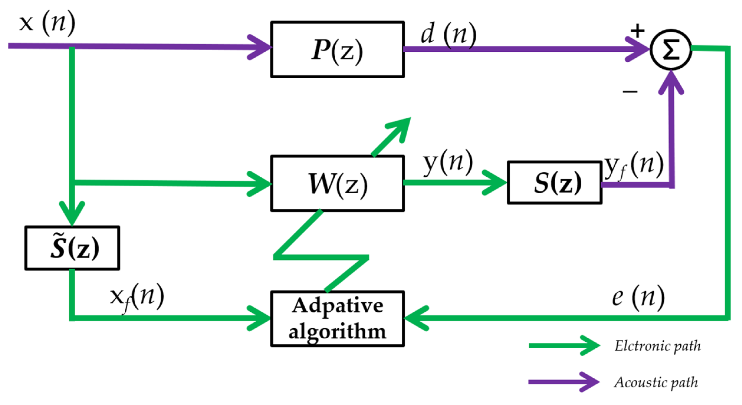
Figure 1. Block diagram of an ANC system using the filtered-x structure.
Applsci 14 01218 g001
Figure 2. Probability density distribution of SαS signals with different intensities.
Applsci 14 01218 g002
Figure 3. α-stable distributed noise signals of different intensities (a) α = 1.8; (b) α = 1.6; (c) α = 1.3.
Applsci 14 01218 g003
Table 1. The characteristics of active noise reduction and passive noise reduction.
CharacteristicsActive Noise ReductionPassive Noise Reduction
Real-timeFaster response and adaptationRelatively slower response
AdaptabilityAutomatically adjusts parametersTypically lacks adaptability
Effective Noise ReductionEffectively suppresses various types of noiseLimited effectiveness in handling complex noise patterns
Power ConsumptionRequires additional powerRelatively lower
power consumption
ComplexityAlgorithm and hardwareMaterial or structure
Relatively simple implementation
Table 2. Summary of adaptive algorithms in Section 2.1.
Cost Function φ ( e ( n ) ) References
J ( n ) = E   [ | e ( n ) | p ] p e ( n ) p sign ( e ( n ) ) [3,4]
J ( n ) = E   [ | e ( n ) | p ] e ( n ) = c 1 i f   e ( n ) c 1 c 2 i f   e ( n ) c 2 e ( n ) c 1 e ( n ) c 2 x f ( n ) = c 1 i f   x ( n ) c 1 c 2 i f   x ( n ) c 2 x f ( n ) c 1 x f ( n ) c 2 p e ( n ) p sign ( e ( n ) ) x f ( n )   [5]
J ( n ) = E   [ | e ( n ) | p ] p | e ( n ) | p 1 sign ( e ( n ) ) / x f ( n ) p p + E ( n ) + δ E ( n + 1 ) = λ E ( n ) + ( 1 λ ) e 2 ( n ) [6,7]
J ( n ) = E   [ | e ( n ) | a q ] p | e ( n ) | a sign ( e ( n ) ) / x f ( n ) a q a q + E ( n ) + δ E ( n + 1 ) = λ E ( n ) + ( 1 λ ) e a q ( n ) a = p β ; q = p / a β [8,9]
J ( n ) = E   [ | e ( n ) | p ] p | e ( n ) | p 1 sign ( e ( n ) ) λ ( n ) ( 1 λ ( n ) ) [ y 1 ( n ) y 2 ( n ) ] [10]
J ( n ) = i = 1 n λ n i log p ( 1 + | e ( n ) | ) φ ( e ( n ) ) = K ( n ) e ( n ) K ( n ) = v ( n ) P ( n 1 ) x s ( n ) λ + v ( n ) x s T ( n ) P ( n 1 ) x s ( n ) P ( n ) = λ 1 P ( n 1 ) λ 1 K ( n ) x s T ( n ) P ( n 1 ) v ( n ) = log p 1 ( 1 + | e ( n ) | ) ( 1 + | e ( n ) | ) | e ( n ) | + τ [11]
Table 3. Summary of adaptive Algorithms in Section 2.2.
Cost Function φ ( e ( n ) ) References
J ( n ) = E   [ | e ( n ) | ] sign ( e ( n ) ) [12,13,19]
J ( n ) = E   [ | e ( n ) | ] sign ( e ( n ) ) sign ( e T ( n ) ) X T ( n ) X ( n ) sign ( e ( n ) ) [14,15]
J ( n ) = E   [ | e ( n ) | ] sign ( e ( n ) ) ( ( 1 β ) μ ( n 1 ) + γ | | p i | | ) p i = β p i 1 + ( 1 β ) sign ( e ( n ) ) x ( n ) [17]
J ( n ) = exp ( e 2 ( n ) δ 2 ) exp ( e 2 ( n ) δ 2 ) sign ( e ( n ) ) V ( n ) V ( n ) = β V ( n 1 ) + ( 1 β ) e 2 ( n ) δ 2 exp ( e 2 ( n ) δ 2 ) [18]
J ( n ) = E   [ | e ( n ) | ] μ ( k ) sign ( e ( n ) ) sign ( e T ( n ) ) X T ( n ) X ( n ) sign ( e ( n ) ) + δ μ ( n ) = α μ ( n 1 ) + ( 1 α ) min [ μ s o l   μ ( n 1 ) ] μ s o l = arg min | | e ( n ) μ ( n ) X ( n ) sign ( e ( n ) ) sign ( e T ( n ) ) X T ( n ) X ( n ) sign ( e ( n ) ) + δ | | 1 [19]
J ( n ) = E   [ | e ( n ) | ] + λ i = 0 M 1 In ( 1 + | w | / ε ) sign ( e ( n ) ) ρ sgn w ( n ) / ( ε + | w ( n ) | ) [20]
J ( n ) = λ ( n ) E   [ e ( n ) p ] + ( 1 λ ( n ) ) E   [ e ( n ) q ] sign ( e ( n ) ) ( λ ( n ) p e ( n ) p 1 + ( 1 λ ( n ) ) p e ( n ) q 1 ) [24]
J ( n ) = 1 2 E   [ log ( 1 + e ( n ) p ) ] d p log ( 1 + e ( n ) ) log ( 1 + | e 2 ( n ) | ) log ( e ( n ) ) e ( n ) sign ( e ( n ) ) [25]
J ( n ) = 1 2 λ n p E   [ e ( n ) p ] d p sign ( e ( n ) ) 1 2 p λ n p e ( n ) p 1 d p [26]
J ( n ) = E   [ | e ( n ) | ] sign ( e ( n ) ) x f ( n ) = q s p n ( n ) x ( n ) q s p n ( n ) = 1 / ( | x ( n ) / r | + 1 ) [27]
Table 4. Summary of adaptive algorithms in Section 3.1.
Cost Function φ ( e ( n ) ) Reference
J ( n ) = E   [ | e ( n ) | 2 ] e ( n ) x f ( n ) x f ( n ) = x f ( n ) x f ( n ) [ c 1 ,   c 2 ] 0 otherwise [29]
J ( n ) = E   [ | e ( n ) | 2 ] e ( n ) x f ( n ) e ( n ) = e ( n ) e ( n ) [ c 1 ,   c 2 ] 0 otherwise   x f ( n ) = x f ( n ) x f ( n ) [ c 1 ,   c 2 ] 0 otherwise [30]
J ( n ) = E   [ | e ( n ) | 2 ] e ( n ) x f ( n ) e ( n ) = sign ( e ( n ) ) ( | e ( n ) | - λ )   e ( n ) [ γ   1 ,   γ   2 ] 0 otherwise x f ( n ) = sign ( x f ( n ) ) ( | x f ( n ) | - λ )   ( x f ( n ) [ γ   1 ,   γ   2 ] 0 otherwise γ = arg m i n ( N + | | x f ( n ) | | + 2 i = 0 N 1   x   n ) [31]
J ( n ) = e 2 ( n ) 2 | e ( n ) | < ξ ξ | e ( n ) | ξ 2 2 ξ | e ( n ) | < Δ Δ 2 2 Δ < | e ( n ) | e ( n ) | e ( n ) | < ξ ζ   sign   (   e ( n )   ) ξ | e ( n ) | < Δ 0   Δ < | e ( n ) | [32]
J ( n ) = c 2 [ e ( n ) c log ( 1 + e ( n ) c ) ] c e ( n ) c + e ( n ) [33]
J ( n ) = e 2 ( n ) 2 | e ( n ) | < ξ ξ | e ( n ) | ξ 2 2 ξ | e ( n ) | < Δ 1 ξ 2 | Δ 2 Δ 1 | ξ 2 2 + ξ 2 ( | e ( n ) Δ 2 | ) 2 Δ 1 Δ 2   Δ 1 | e ( n ) | < Δ 2 Δ 2 2 2   Δ 2 < | e ( n ) | e ( n ) | e ( n ) | < ξ ζ   sign ( e ( n ) ) ξ | e ( n ) | < Δ 1 ξ 2 ( | e ( n ) Δ 2 | ) Δ 1 Δ 2   Δ 1 | e ( n ) | < Δ 2 0   Δ 2 < | e ( n ) | [34]
J ( n ) = e 2 ( n ) 2 | e ( n ) | < ξ ξ | e ( n ) | ξ 2 2 ξ | e ( n ) | < Δ 1 ξ 2 | Δ 2 Δ 1 | ξ 2 2 + ξ 2 ( | e ( n ) Δ 2 | ) 2 Δ 1 Δ 2   Δ 1 | e ( n ) | < Δ 2 Δ 2 2 2   Δ 2 < | e ( n ) | x   ( n ) 0   | x   ( n ) |     ξ ξ   s i g n   [ x   ( n ) ] ξ < | x   ( n ) |     Δ 1 [   (   | x   ( n ) | Δ 2 ) ξ Δ 1 Δ 2 ]   s i g n   [ x   ( n ) ] Δ 1 < | x   ( n ) |     Δ 2 0 Δ 2 < | x   ( n ) | [35]
Table 5. Summary of adaptive algorithms in Section 3.2.
Cost Function φ ( e ( n ) ) References
J ( n ) = E   [ log 2 e ( n ) ] log ( e ( n ) ) sign ( e ( n ) ) e ( n ) [36]
J ( n ) = E   [ log [ 1 + e 2 ( n ) 2 δ 2 ] ] e ( n ) e 2 ( n ) + 2 δ 2 [37]
J ( n ) = E   [ f ( e ( n ) ) ] 1 α E [ log [ 1 + α f ( e ( n ) ) ] ] f ( e ( n ) ) = e ( n )   ( L L A D ) α e ( n ) 1 + α | e ( n ) |         ( L L A D ) [38]
J ( n ) = n i = 1 λ n i log [ 1 + | e ( n ) | p ] n i = 1 λ n i p e ( n ) p 1 s i g n ( e ( n ) ) 1 + e ( n ) p [39]
J ( n ) = M 1 i = 1 log [ 1 + ( e ( i ) δ ) 2 ] n i = 1 λ n i e ( i ) δ 2 + e 2 ( i ) [40]
J ( n ) = E   [ In [ cosh ( λ | e ( n ) | p ) ] ] tanh ( ρ e ( n ) ) [41,42,43,44,50]
J ( n ) = 1 β tanh ( β 2 ( e ( n ) x ( n ) ) 2 ) 4 exp ( β ( e ( n ) / x ( n ) ) 2 e ( n ) ( 1 + exp ( β ( e ( n ) / x ( n ) ) 2 ) x ( n ) ) 2 [45]
J ( n ) = E   [ sech ( e 2 ( n ) ) λ 2 e 2 ( n ) ] e ( n ) sech ( e 2 ( n ) ) tanh ( e 2 ( n ) ) + λ e ( n ) [46]
J ( n ) = E   [ 1 λ tanh ( λ | e ( n ) | p ) ] p | e ( n ) | p 1 sech ( λ | e ( n ) | p ) sign ( e ( n ) ) [47]
J ( n ) = E   [ sech ( λ | e ( n ) | p ) ] p sech ( λ | e ( n ) | p ) tan ( λ | e ( n ) | ) [48]
J ( n ) = 4 k π arctan ( π k 2 e ( n ) ) 32 arctan ( π k 2 e ( n ) ) π 4 k 2 e 2 ( n ) + 4 π 2 [49]
J ( n ) = 1 E   [ γ exp [ cosh ( λ | e ( n ) | p ] ] exp [ cosh ( λ | e ( n ) | 2 sinh ( 2 λ | e ( n ) | ) (p = 2) [51]
J ( n ) = 1 E   [ exp [ sinh 2 ( λ e ( n ) ] ] exp [ sinh 2 ( λ e ( n ) ] sinh ( 2 λ e ( n ) ) [52]
J ( n ) = E   [ sinh 1 ( | e ( n ) | 2 ) ] e 2 ( n ) 1 + e 2 ( n ) [53]
Table 6. Summary of adaptive algorithms in Section 4.
Cost Function φ ( e ( n ) ) References
J ( n ) = exp ( e 2 ( n ) 2 δ 2 ) exp ( e 2 ( n ) 2 δ 2 ) e ( n ) δ 2 [54,55,56,61]
J ( n ) = exp ( ( e ( n ) β ) a ) exp ( ( e ( n ) β ) a ) a e ( n ) a 1 β a [57]
J ( n ) = i = 1 n λ n i exp ( e 2 ( n ) / 2 δ 2 ) i = 1 n λ n i exp ( e 2 ( n ) / 2 δ 2 ) e ( n ) / 2 δ 2 [58]
J ( n ) = i = 1 n λ n i exp ( e 2 ( n ) / 2 δ 2 ) α ( n ) p ( n ) α ( n ) = g T ( n ) p ( n ) p T ( n ) R ( n ) p ( n ) R ( n ) = R ( n 1 ) + exp ( e 2 ( n ) / 2 δ 2 ) r ( n ) r T ( n ) p ( n ) = ( 1 + β ( n ) g T ( n ) p ( n 1 ) g T ( n ) g ( n ) ) g ( n ) + β ( n ) p ( n 1 ) β ( n ) = g T ( n ) ( g ( n ) g ( n 1 ) ) g T ( n 1 ) g ( n 1 ) g ( n ) = g ( n 1 ) α ( n ) R ( n ) p ( n )   + exp ( e 2 ( n ) / 2 δ 2 ) r ( n ) ( d ( n ) W T ( n ) s ( n ) * x ( n ) ) r ( n ) = s ( n ) * x ( n ) [62]
J ( n ) = exp ( λ ( 1 exp ( e 2 ( n ) 2 δ 2 ) ) ) λ exp ( λ ( 1 exp ( e 2 ( n ) 2 δ 2 ) ) ) exp ( e 2 ( n ) 2 δ 2 ) e ( n ) δ 2 [63,64]
J ( n ) = 1 2 γ E   [ 1 1 + γ | e ( n ) | p ] ] | e ( n ) | p 1 sign ( e ( n ) ) ( 1 + γ | e ( n ) | p ) 2 [66,67,68]
J ( n ) = 1 γ E   [ 1 1 + exp ( γ | e ( n ) | 2 ) ] 2 e ( n ) 1 + exp ( γ | e ( n ) | 2 ) ( 1 1 1 + exp ( γ | e ( n ) | 2 ) ) [70]
J ( n ) = E   [ 1 + λ | e ( n ) | 2 ] 1 exp ( ( e ( n ) β ) a ) a e ( n ) a 1 β a [71]
Disclaimer/Publisher’s Note: The statements, opinions and data contained in all publications are solely those of the individual author(s) and contributor(s) and not of MDPI and/or the editor(s). MDPI and/or the editor(s) disclaim responsibility for any injury to people or property resulting from any ideas, methods, instructions or products referred to in the content.