Article

Carbon Quota Allocation Prediction for Power Grids Using PSO-Optimized Neural Networks

1
College of Management, Shenyang Jianzhu University, Shenyang 110168, China
2
School of Economics and Management, Beijing Jiaotong University, Beijing 100044, China
3
School of Materials Science and Engineering, Northeastern University, Shenyang 110819, China
4
International College, Shenyang Jianzhu University, Shenyang 110168, China
5
School of Materials Science and Engineering, Shenyang University of Technology, Shenyang 110870, China
6
School of Engineering, Design and Built Environment, Western Sydney University, Penrith, NSW 2751, Australia
7
Centre for Infrastructure Engineering and Safety, School of Civil and Environmental Engineering, The University of New South Wales, Sydney, NSW 2052, Australia
*
Authors to whom correspondence should be addressed.
Appl. Sci. 2024, 14(24), 11996; https://doi.org/10.3390/app142411996
Submission received: 16 November 2024 / Revised: 13 December 2024 / Accepted: 20 December 2024 / Published: 21 December 2024
(This article belongs to the Special Issue Artificial Intelligence Applications in Smart Energy Systems)

Abstract

:
Formulating a scientifically sound and efficient approach to allocating carbon quota aligned with the carbon peaking goal is a fundamental theoretical and practical challenge within the context of climate-oriented trading in the power sector. Given the highly irrational allocation of carbon allowances in China’s power sector, as well as the expanding role of renewable energy, it is essential to rationalize the use of green energy in the development of carbon reduction in the power sector. This study addresses the risk of “carbon transfer” within the power industry and develops a predictive model for CO2 emission based on multiple influential factors, thereby proposing a carbon quota distribution scheme adapted to green energy growth. The proposed model employs a hybrid of the gray forecasting model-particle swarm optimization-enhanced back-propagation neural network (GM-PSO-BPNN) for forecasting and allocating the total carbon quota. Assuming consistent total volume control through 2030, carbon quota is distributed to regional power grids in proportion to actual production allocation. Results indicate that the PSO algorithm mitigates local optimization constraints of the standard BP algorithm; the prediction error of carbon emissions by the combined model is significantly smaller than that of the single model, while its identification accuracy reaches 99.46%. With the total national carbon emissions remaining unchanged in 2030, in the end, the regional grids received the following quota values: 873.29 million tons in North China, 522.69 million tons in Northwest China, 194.15 million tons in Northeast China, 1283.16 million tons in East China, 1556.40 million tons in Central China, and 1085.37 million tons in the Southern Power Grid. The power sector can refer to this carbon allowance allocation standard to control carbon emissions in order to meet the industry’s emission reduction standards.

1. Introduction

In recent years, China’s power industry has become the largest source of global carbon dioxide emissions, with coal-fired power generation contributing the most to its greenhouse gas emissions. Amid the global energy transition, renewable energy power generation has emerged as a crucial pathway toward achieving a green, low-carbon transition and net-zero emissions. Riding the momentum of the “double carbon” policy, the renewable energy sector has entered a golden period of development, especially wind and solar energy, which will hold a leading position in the future energy generation market [1,2]. In December 2017, the comprehensive CO2 emissions trading system in China was officially launched, with the power segment as the first and only industry to be included. The allocated CO2 emission allowances in China are crucial for the establishment of a national carbon market trading mechanism and the realization of China’s 2030 carbon peaking target. The CO2 emissions trading system is an effective vehicle to reduce carbon emissions through market mechanisms [3,4]. The primary starting points for existing researchers’ research on quota allocation are efficiency and equity. The issue of equity is considered extremely critical in international climate negotiations [5]. There is no single definition of equity that is universally accepted, and the principle of equity refers to a more general concept of distributive justice or fairness [6]. Based on the principle of equity, Pozo et al. [7] applied it to the allocation of global CO2 quotas based on three dimensions: responsibility, capacity, and equity. The carbon sink attribute of agriculture is considered and characterized as a safeguard-type equity indicator in light of the somewhat increased theoretical bounds of carbon emissions [8]. Cost-effectiveness and input-output effectiveness are the two metrics typically employed to assess the efficiency principle. As far as efficiency is concerned, cost-effectiveness refers to the minimization of the gross abatement cost. Jiang et al. [9] allocated CO2 allowances from a cost-negligible perspective. Among the input-output criteria, DEA is the most frequently used approach to evaluate the efficiency of CO2 emissions. Cai and Ye [10] employed the data envelopment analysis (DEA) model for the efficient allocation of CO2 emission allowances. Fang et al. [11] introduced the carbon emissions trading system (ETS), and a valuation model for emission quota options under the ETS was introduced, it was found that the price of allowance options exhibited volatility similar to that of the stock market. Initially, power companies participated in the ETS through the free allocation of carbon emission allowances (EUAs), raising concerns about windfall profits for producers with carbon-intensive power portfolios. To address this issue, the transition of the trading model to an auction-based allocation at the beginning of the third phase of the ETS was designed to eliminate this discrepancy. However, the interaction between power generation and consumption complicates the quantitative analysis of carbon emission responsibility [12]. Additionally, the use of single-indicator predictions to determine total carbon allowance allocations often results in unfair and unreasonable outcomes. Therefore, it is essential to compute total carbon quota allocations taking into consideration the effect of renewable energy power generation on the system so as to improve the formulation of CO2 emission credits in the electricity system under the carbon trading market. Additionally, establishing an equitable and rational allocation plan that takes into account the interactions between power consumption and generation regions is essential.

2. Literature Review

As a key industry in the study of global CO2 emissions, analyzing the current status of power sector emissions is essential for developing effective emission reduction strategies. Power-related carbon emissions issues have been the focus of much research in recent years by numerous academics, who have concentrated on both the types of emission generation and the factors that influence them. The emissions from the power sector can be categorized into direct emissions from electricity generation and indirect emissions from electricity demand [13]. Von et al. [14] proposed a method for calculating carbon emissions based on electricity consumption, while Qu et al. [15] used a network approach to estimate carbon emissions from electricity consumption in 137 countries and regions around the world. Zhang et al. [16] and Wei et al. [17] utilized various methods, including the carbon inventory approach and multi-region input-output approach, to calculate electricity-related carbon emissions. Greenhouse gas emissions from China’s cross-provincial electricity trading were examined by Li et al. [18]. The influence of shifting electricity sources on carbon accounting was investigated by Eberle and Heath [19]. Lopez et al. [20] studied the effect of energy trading on CO2 emissions in the top 20 electricity trading nations in Europe. Li et al. [21] looked at the effects of power trading on air quality in the Yangtze River Basin. Similarly, Ehigiamusoe [22] compared the impact of electricity trade on CO2 emission changes with other key factors, including energy intensity and economic performance. Xu et al. [23] conducted a temporal and spatial decomposition study on the factors driving CO2 emission changes in China’s thermal power industry from 2010 to 2020, revealing regional variability and trends in emission dynamics by expanding the Kaya constant equation and applying the LMDI decomposition method.
Establishing an effective carbon emission prediction model (CEPM) to understand and forecast carbon dioxide emission trends is essential for mitigating climate change. Forecasting domestic and international carbon emissions from electricity relies primarily on quantitative methods, encompassing both individual and integrated forecasting models, including artificial neural networks, genetic algorithms, support vector machines, linear regression, and the GM(1,1) model [24]. Zuo et al. [25] presented continuous emission monitoring systems and predictive emission monitoring systems commonly utilized in power plants and highlighted that machine learning techniques are capable of significantly improving predictive emission monitoring systems via their ability to intelligently deal with large data sets, thereby transforming traditional emission monitoring systems by increasing the accuracy, effectiveness, and cost-efficiency. Jin et al. [26] reviewed 147 CEPMs and noted the increasing use of neural network models, particularly feed-forward architectures, with many models incorporating meta-heuristic approaches. Parameter optimization was the main focus of prediction algorithms, followed by structural optimization. Predictor selection models employed grey relational analysis and principal component analysis for statistical and machine learning applications, effectively filtering influencing factors. Wang et al. [27] constructed a new optimization model OGMW(1,1) based on the GM(1,1) model to predict a trend of China’s primary sources of energy, oil and coal consumption, and CO2 emission in the next five years. Zhao et al. [28] proposed a random forest regression model enhanced by a genetic learning strategy to improve the traditional artificial bee colony algorithm for predicting CO2 emissions in the power system. Li and Zhang [29] addressed the issues of outliers and heteroskedasticity by applying a grey theory prediction model with nonlinear inflection point forecasting. While machine learning algorithms perform well in short-term data prediction, they often require extensive high-dimensional data. Many scholars have confirmed that combined prediction models outperform single models by integrating grey theory and neural networks. Meanwhile, during the learning process of neural networks, existing scholars usually combine other algorithms with them to improve the prediction accuracy. Some scholars have combined neural networks with particle swarm optimization algorithms to build PSO-BP prediction models [30,31]. Hu [32] developed the NNGM(1,1) model, a combination of grey theory and neural networks, and applied it to forecast electricity consumption using data from the Ministry of Energy and Natural Resources of Turkey and the Asia-Pacific Economic Cooperation. Chiang et al. [33] proposed an adaptive electricity load forecasting method by fusing neural networks with grey modeling, leveraging the complementary strengths of both techniques. Wang et al. [34] employed a combination of particle swarm optimization, genetic algorithms, and BPNN models to forecast shallow groundwater levels in Harbin. Liu and Shao [35] devised a sparrow search algorithm-particle swarm optimization-back-propagation neural network (SSA-PSO-BPNN) model to precisely anticipate the deformation of aerospace wall plates during clamping. Zheng et al. [36] used the STIRPAT-GA-BPNN model optimized by a genetic algorithm to analyze the scenario prediction of the maximum CO2 emission in Dalian, China, and the accuracy of the predicted carbon emissions was as high as 99.33%, which proved its excellent prediction ability. Yang et al. [37] proposed a technique that uses PSO in combination with the fusing of a one-dimensional convolutional neural network (CNN) and a multi-head self-attention (MHSA) bidirectional long short-term memory (BiLSTM) network called PSO-CNN-BiLSTM-MHSA. Ellahi et al. [38] used a combination of particle swarm optimization algorithms as well as bat algorithms to obtain the hybrid particle swarm optimization (PSO) and a Bat algorithm (BA) (HPSOBA) and accurately predicted wind speeds and wind energy using cascaded feed-forward neural networks.
The Carbon Emissions Trading Scheme (ETS) has significantly improved the pollution and CO2 reductions of China’s power sector, especially in terms of effective synergies in reducing CO2, SO2, and PM2.5 emissions [39]. Jin et al. [40] demonstrated that carbon trading improves carbon emission efficiency using an uncertainty-related stochastic DEED model. Wang et al. [41] formulated a PEQ-based carbon quota allocation model for coal power supply chain enterprises. Meng et al. [42] employed a combined trend prediction model and a triple-index allocated model for analyzing the provincial CO2 emission allowance distribution of China’s power system. Meanwhile, Wang et al. [43] employed the Zero-Sum-Gain Data Envelopment Analysis model to construct a multi-criteria carbon quota allocation system for the power sector and utilized the CO2 emission flow (CEF) model to track the “virtual” carbon flows in conjunction with electricity flows. Ma et al. [44] designed a planning model to allocate carbon reduction shares among China’s five largest power companies and evaluated their efficiency using the zero-sum gain data envelopment analysis (ZSG-DEA) method. Zhang et al. [45] established a Computable General Equilibrium (CGE) model to study China’s electric power carbon allowance allocations and found that using historical emissions as a benchmark for quota allocation leads to better outcomes. Lyu et al. [46] developed a cross-regional electricity trading cooperation game model, finding that shared responsibility between producers and consumers for carbon quotas is more effective than placing the responsibility solely on producers, especially when low-carbon policies on the demand side are relaxed. Regarding renewable energy’s impact on electricity carbon quotas, Zhu et al. [47] found that the green label price under the Renewable Energy Certificate (REC) policy has a non-monotonic impact on investment in renewable energy, influenced significantly by the quota set under the Renewable Energy Standard (RES) policy. Li et al. [48] developed a carbon transaction cost model for wind and thermal energy and adopted a carbon quota distribution strategy that used the entropy weight method to adjust the proportions of benchmark emission components in regional power systems.
The majority of current research on carbon allocation in the power industry focuses primarily on thermal power generation, with little attention paid to the impact of renewable energy on emissions. This is based on both domestic and international research on the influence of CO2 emissions from electricity, the determination of total carbon quota allocations, and allocation methods. Furthermore, the determination of total carbon quotas often relies on a single factor, overlooking the potential risk of “carbon transfer” within the power industry, leading to allocation schemes that lack fairness. To address these gaps, this study builds a carbon emissions impact indicator system for the power sector and improves the current prediction model by using the PSO algorithm, which gets around the drawbacks of conventional neural networks in global optimization. In an attempt to identify a more accurate carbon emissions forecasting model under the effect of several factors, the paper combines the GM(1,1) gray prediction model with BPNN. The forecasting precision of the synthesized model is compared with that of the standalone GM(1,1) model. With the total carbon emission control unchanged by 2030, the shared emission reduction responsibility coefficient is introduced to address the challenge of dividing emission reduction responsibilities within the power system. This allows for a quantitative analysis of the emission reduction responsibilities of each regional power grid, ensuring a fair allocation of carbon quotas and facilitating the proposal of reasonable and effective emission reduction measures based on the quota standard.

3. Materials and Methods

3.1. Status of Carbon Emissions in the Power Sector

Carbon footprints in the power sector come mainly from power plants. The primary forms of power generation include wind, thermal, hydroelectric, solar, and nuclear. Thermal power stands as a predominant contributor to CO2 emissions; thus, we focus our CO2 emissions calculations on thermal power generation.

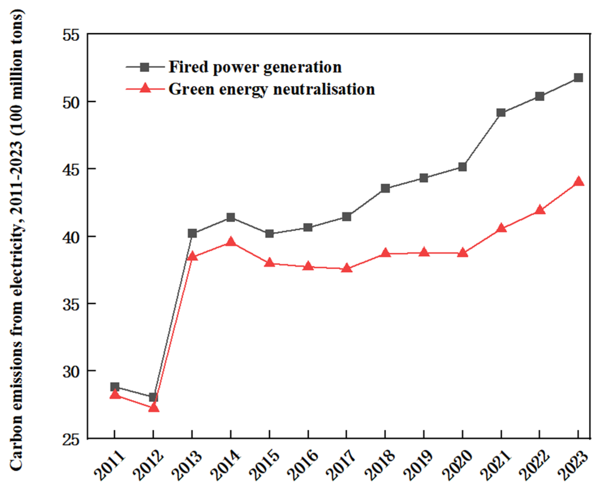
3.1.1. CO2 Emission Measurement in the Power Sector

  • Thermal power generation CO2 emissions
The IPCC methodology was developed by the Intergovernmental Panel on Climate Change (IPCC) to account for emissions from electricity generation and is the most widely used methodology in the world (IPCC, 2006) [17]. Since power plants are the main source of carbon emissions in the power sector, power generation capacity is used as a quantitative indicator to measure these emissions. The mathematical expression for carbon emission calculation from coal-fired power generation for the period 2021–2023 is as follows:
E M f = E f i r × E C E F
where E M f represents carbon emissions from thermal power (billion ton), E f i r represents thermal power generation ( k w h ), and E C E F represents carbon emission factors for electricity in each region ( k g / k w h ).
2.
Green energy neutralizes carbon emissions
Since green energy does not produce carbon dioxide during power generation, it helps reduce some of the emissions associated with thermal power generation. Therefore, this paper uses the electricity generated by green energy, both during and after its integration (collectively referred to as the electricity generated in and after green energy), as the quantitative indicator of green energy generation. Similarly, the carbon emissions from green energy and the corresponding portion of thermal power generation (collectively referred to as the carbon emissions from green energy in and after green energy) are used as the indicators of emissions after the influence of green energy. The green energy neutralization and post-carbon emissions for 2021–2023 are then measured using Equations (2) and (3):
G e = ( E f i r E g r e )
E M g = G e × E C E F
where G e represents green energy neutralization generation (kWh), and E g r e represents renewable energy generation (kWh). E M g represents post-neutral green energy (100 million tons).
Analyses of the past decade based on electricity sector CO2 emissions measured from 2012 to 2023 show a continuous increase in CO2 emissions from the electricity sector (Figure 1). However, as carbon emissions are affected by electricity output and CO2 emission factors, the trend is unstable, rising sharply at times and falling sharply at others. The data for this analysis is sourced from the (2012–2024) China Electricity Statistical Yearbook.

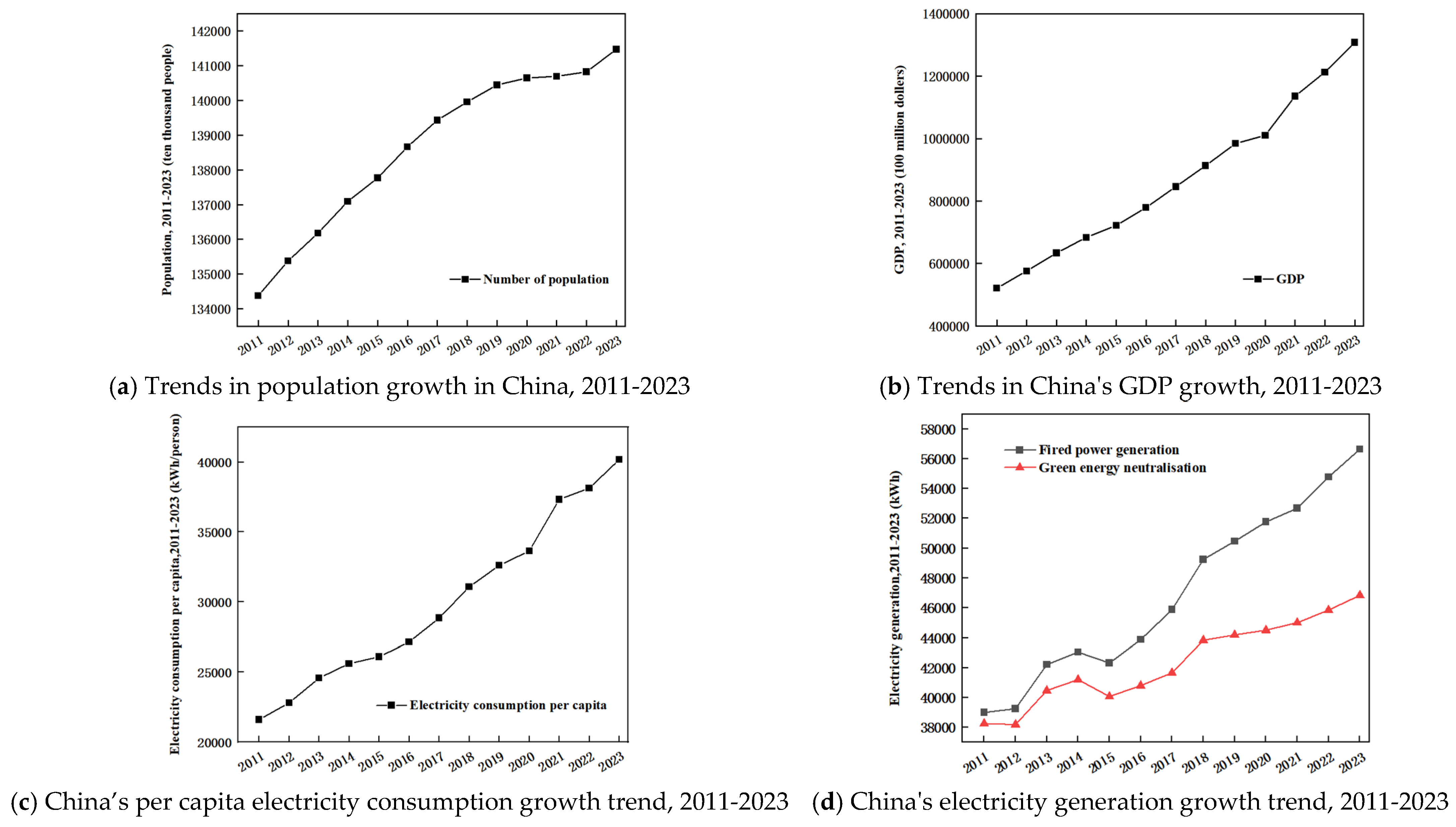
3.1.2. Indicator Characteristics

It was found that factors including population size, economic development, and energy intensity have a great bearing on the carbon emission drive of China’s electricity consumption, in which thermal power generation, historical accumulated CO2 emissions, and carbon strength indicators are suitable to be used as impact indicators for allocating electricity carbon allowances [49,50]. In this paper, the factors influencing carbon emissions in the power sector are categorized into three key indicators: emission abatement responsibility, emission abatement potential, and emission abatement capacity, forming a multi-indicator comprehensive evaluation system. These indexes are summarized in Table 1.
Based on the multi-indicator comprehensive evaluation system, the analysis of carbon emission indicators in the power industry from 2012 to 2023 reveals several trends: population, per capita electricity consumption, and GDP have all shown consistent growth, although population growth slowed between 2020 and 2021. Power generation in the industry has generally increased, with thermal power generation following a continuous upward trend. However, green power generation has experienced a fluctuating upward trend due to factors such as regional restrictions and immature technology, with occasional declines in certain years (e.g., Figure 2). The data for this analysis is sourced from the 2012–2024 China Statistical Yearbook.

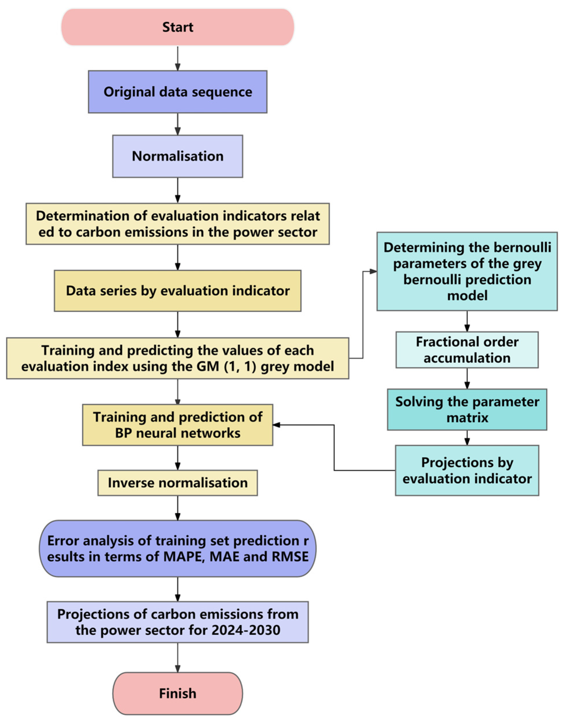
3.2. Model Building and Optimization

Grey prediction models and machine learning methods are commonly utilized for predicting time series data, especially when dealing with small sample sizes and long-term prediction. In this research, a hybridized prediction model combining GM(1,1) and BPNN is developed to predict CO2 emissions in the electric power system from 2024 to 2030, forming the basis for the regional allocation scheme of carbon allowances. The model comprises two components: the GM(1,1) module and the BPNN module. Based on analyzing carbon emission-related impact indicators, which demonstrate a consistent growth trend, the GM(1,1) model is applied to forecast these indicators in the electric power industry. However, due to the fluctuating growth pattern of historical carbon emissions, the prediction accuracy of the GM(1,1) model decreases and fails to capture the complicated relationship between the indicators and carbon emissions. To address this limitation, the BPNN model is employed to predict the CO2 emission of electric power systems in China.
In this paper, using the GM(1,1) model, based on the concept of grey generating function with differential fitting as the core, the indicator values are substituted into the function to find grey Bernoulli parameter values, but rather the haphazard column of the original carbon emission indicator data into a more regular time series data, the establishment of a dynamic model to obtain the predicted value of the carbon emission indicator, the carbon emission is an extremely unstable indicator, cannot be carried out singularly. Carbon emissions are an extremely unstable indicator, which cannot be predicted singly, so the output value generated by GM(1,1) is used as the input value of the PSO-BP neural network, and machine learning is utilized to iterate and train the model, and the prediction accuracy of the carbon emissions is finally measured by the training error indicator, which provides reliable basic data for the allocation of carbon quotas in the later stage. The flowchart of the proposed hybridized prediction model can be found in Figure 3.

3.2.1. GM(1,1) Module

GM(1,1) is an effective tool to deal with small sample prediction problems. When dealing with fewer eigenvalue data, the model does not need the sample space of the data to be large enough to solve the problems of small historical data, low sequence integrity, and unreliability. GM(1,1) transforms the irregular raw data into a more regular generating sequence through the methods of cumulative generation, cumulative subtraction generation, mean generation, rank-ratio generation, and so on. It is especially suitable for the prediction problem that approximates the exponential growth, so GM(1,1) has superiority in prediction [51]. Since the historical data related to CO2 emission in the power industry are less and the CO2 emission shows a yearly growth trend, the model is used to predict the aggregate quantity of carbon quota distribution, and the concrete steps are as follows:
  • Processing of raw carbon emissions data
This process involves cumulative generation, transforming the original data to create new sequences that enhance the level of smoothing and stability of the data. Assuming the original sequence of carbon emission-related indicators for the power industry is as follows:
X ( 0 ) = [ x ( 0 )   ( 1 ) , x ( 0 )   ( 2 )   , x ( 0 )   ( 3 ) , x ( 0 )   ( n ) ]
where X ( 0 ) is the original time series of carbon emissions from the power industry, x ( 0 )   ( 1 ) , x ( 0 )   ( 2 )   , x ( 0 )   ( 3 ) , x ( 0 )   ( n ) are the original carbon emissions data of each carbon source, respectively.
A new carbon emission sequence X ( 1 ) is generated by accumulating Equation (4).
X ( 1 ) = [ x ( 1 )   ( 1 ) , x ( 1 )   ( 2 )   , x ( 1 )   ( 3 ) , x ( 1 )   ( n ) ]
x ( 1 ) ( k ) = n = 1 k x ( 0 ) ( n )
where X ( 1 ) is the cumulative generation of new carbon emissions time series   x ( 1 )   ( 1 ) , x ( 1 )   ( 2 )   , x ( 1 )   ( 3 ) , x ( 1 )   ( n ) is the cumulative carbon emissions data for each indicator x ( 1 ) ( k ) is the cumulative value between the original data.
2.
Construction of GM(1,1) primitive form. Assuming that   X ( 1 ) has an approximate exponential variation rule, then x ( 1 ) ( k ) can be regarded as a function of time t x ( 1 ) ( k ) = x ( 1 ) ( t ) , then, the whitened form of GM(1,1) is as follows:
x ( 0 )   ( k ) = d x ( 1 ) ( k ) = x ( 1 ) ( k ) x ( 1 ) ( k 1 ) z ( 1 ) ( k ) = 0.5 x ( 1 ) ( k ) + 0.5 ( k 1 ) x ( 1 )
The white differential equation for its GM(1,1) is:
d x ( 1 ) ( k ) / d t + a x ( 1 ) ( k ) = b
where x ( 0 ) ( k ) is the grey derivative corresponding to x ( 1 ) ( k ) ; a is the development coefficient; b is the amount of grey action; z ( 1 ) ( k ) is the whitening background value corresponding to x ( 1 ) ( t ) .
Then, the original form of GM(1,1) is as follows:
x ( 0 ) ( k ) / d t + a z ( 1 ) ( k ) = b
3.
Establishment of the data matrix and data vector of the grey Bernoulli prediction model for carbon emissions. In the calculation process, it is common to use Z and X to represent the matrices.
Z = z ( 1 ) ( 2 ) z ( 1 ) ( 2 ) r z ( 1 ) ( n ) z ( 1 ) ( n ) r
X = x ( 0 ) ( 2 ) x ( 0 ) ( n )
The parameter matrix of the grey Bernoulli prediction model can be found by the least squares method as follows:
a , b T = B T B 1 B T Y
4.
Construct the time-response function and calculate the predicted values
The time response function can be introduced by bringing the parameter matrix into the grey differential equation:
x ( 1 ) ( k + 1 ) = ( x ( 0 ) ( 1 ) b / a ) a k + b / a
x ( 0 ) ( k + 1 ) = x ( 1 ) ( k + 1 ) x ( 1 ) ( k )
where x ( 1 ) ( k + 1 ) is the predicted value of the cumulative data for carbon emissions; x ( 0 ) ( k + 1 ) is the predicted value of each carbon source corresponding to the reduced cumulative value x ( 1 ) ( k + 1 ) ; and x ( 0 ) ( 1 ) is the raw data for the carbon emissions corresponding to the first carbon emission targets.
5.
Accuracy test of carbon emission projections
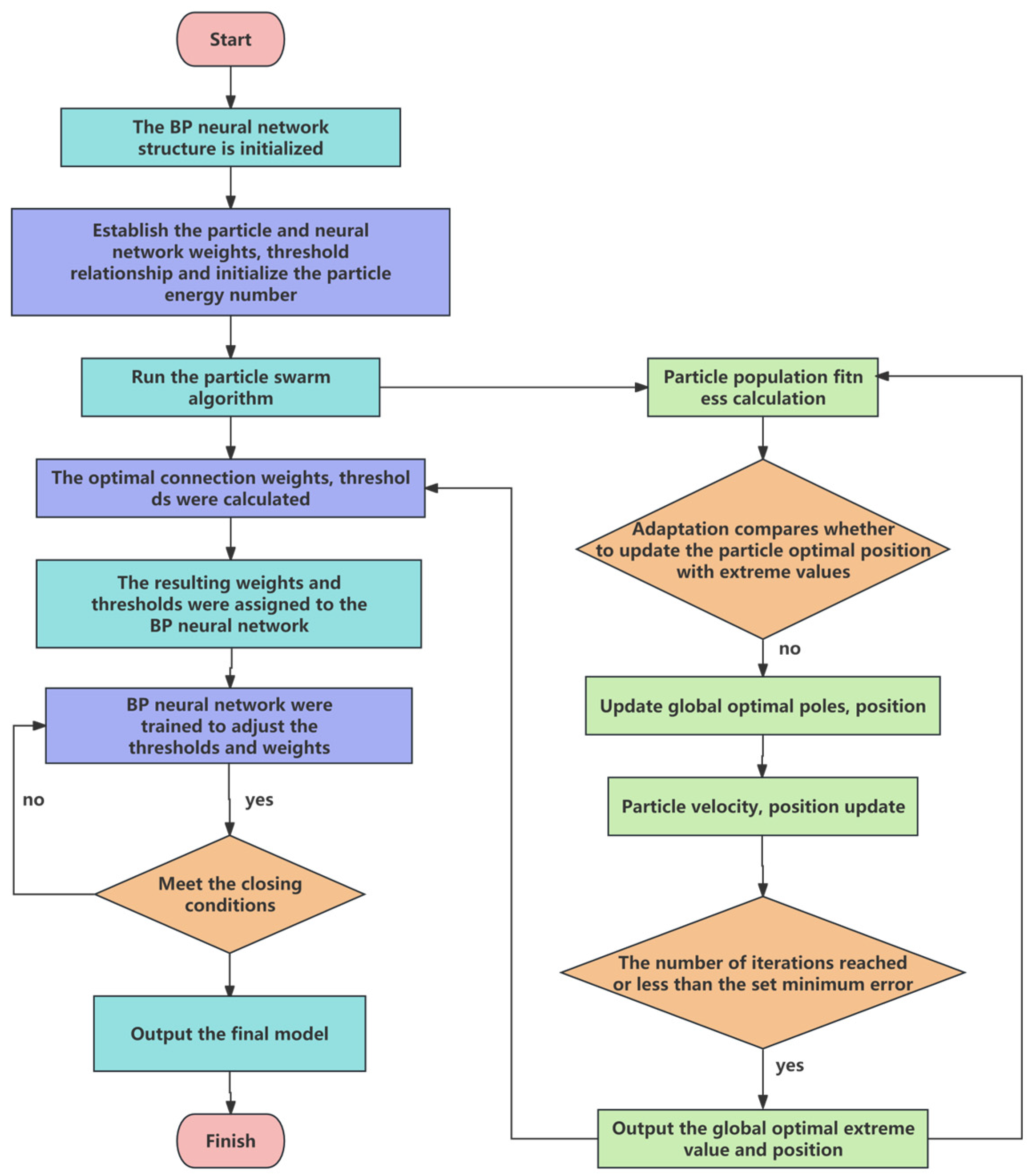
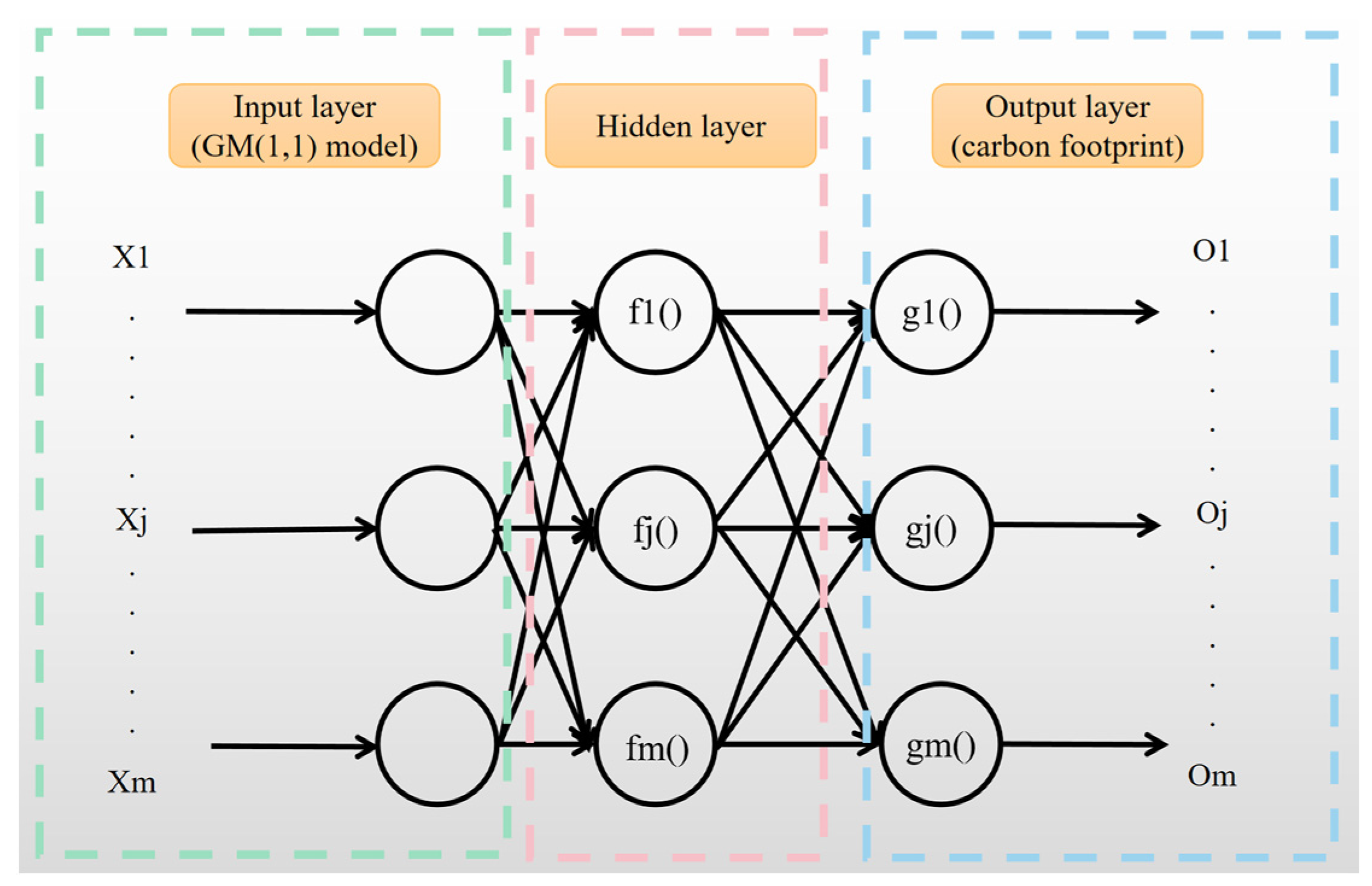
ε ( k ) = [ x ( 0 ) ( n ) x ( 0 ) ( k + 1 ) ] / x ( 0 ) ( k + 1 )
where ε ( k ) is the model residual value; x ( 0 ) ( n ) is the true value; x ( 0 ) ( k + 1 ) is the predicted value. In this case, if ε ( k ) < 0.2 , it can be considered to meet the general requirements; if ε ( k ) < 0.1, it can be considered to meet the higher requirements.

3.2.2. BPNN Module

In the mid-1980s, Rumelhart [52] proposed the well-known error back propagation (BP) as a now commonly used machine learning method suitable for constructing multi-layer orthogonal networks and training them with a back propagation algorithm to minimize the difference between the output and the real value. The algorithm is effectively used as an excellent fitting function for practical problem solving such as regression analysis and classification tasks [53].
  • Neural network algorithm flow
The specific process of neural network establishment is as follows:
Step 1: Determine the input dimension based on the input sample, and set up the input layer. The activation function is configured as the Sigmoid function, expressed as follows:
g ( x ) = 1 / ( 1 + e x )
Step 2: Output of the hidden and output layers
The BPNN typically consists of three layers: the input layer (representing the output set of the GM(1,1) model), the hidden layer, and the output layer (representing the carbon emissions from the power sector), as shown in Figure 4. Let the number of nodes in the input, hidden, and output layers be denoted as m, n, and s, respectively.
The hidden layer output formula is shown in (17):
H k = f i = 1 m x i · w i k a k
where i = 1,2 , . . . , m ; k = i = 1,2 , . . . , n ; w i k is the link weight coefficient from the input layer to the hidden layer and a k   is the bias.
The mathematical expression for the output layer is shown in (18):
O j = i = 1 m H k · w k j b j
where j = 1,2 , . . . , s ; w k j is the connection weight coefficient from the hidden layer to the output layer and b j is its bias.
Step 3: Calculate the error. The error is the difference between the output of the input layer and the desired output, as expressed in Formula (19):
e j = O j O j
where j = 1,2 , . . . , s ; O j denotes the desired output value and O j is the true value.
Step 4: Weight updating. The formula for updating connection weights from the input layer to the hidden layer is provided in Equation (20):
w i k = w i k + θ H k 1 H k · x i i = 1 m e j · w k j
The formula for updating the threshold from the hidden layer to the output layer is given in Equation (21):
w k j = w k j + θ H k · e j
where i = 1,2 , . . . , m ; k = i = 1,2 , . . . , n ; j = 1,2 , . . . , s .
Step 5: Update threshold
The formula for updating the threshold from the input layer to the hidden layer is shown in (22):
a k = a k + θ H k 1 H k i = 1 m e j · w k j
The threshold update formula for the implicit layer to the output layer is shown in (23):
b j = b j + e j
where i = 1,2 , . . . , m ; k = i = 1,2 , . . . , n ; j = 1,2 , . . . , s .
Step 6: Judge the termination condition
If the error e j falls within a reasonable range, the calculation will terminate; otherwise, the hidden and output layers will be recalculated, returning to step 2.
2.
PSO optimization algorithm
PSO is a heuristic search method that mimics the foraging behavior of birds [54,55]. To address the issue of local optima that the BP neural network tends to encounter during the learning process, this paper incorporates the PSO algorithm to perform a global search for the optimal initial weights and thresholds of the BP neural network. This approach helps the BP neural network escape from local extrema.
The PSO algorithm regards the solution of optimal problems as searching for optimal particles in a D-dimensional space. The total number of particles in the population is u, vector r i = [ r i 1 , r i 2 , . . . , r i D ] T indicates the position of the ith particle, vector v i = [ v i 1 , v i 2 , . . . , v i D ] T   represents the velocity of the ith particle, vector k i = [ k i 1 , k i 2 , . . . , k i D ] T represents the optimal position searched by the particle itself, vector g i = [ g i 1 , g i 2 , . . . , g i D ] T   represents the optimal location searched for the entire population, z is the particle numbering, z ( 1,2 , , u ) .
The velocity and position of the PSO are expressed by the following equation: Initially, the PSO algorithm calculates the fitness value of each particle using the fitness function and iteratively updates it to search for the optimal solution. In each iteration, particle   r i   updates its position and velocity based on its individual optimal value k i and the global optimal value   g z .
The velocity and position of the particles in PSO are expressed by the following equations.
v i ( n + 1 ) = w v i ( n ) + c 1 r a n d ( x ) [ k i ( n ) r i ( n ) + c 2 r a n d ( x ) [ g z r i ( n ) ]
r i ( n + 1 ) = r i ( n ) + v i ( n + 1 )
where n is the number of iterations; w is the inertial weight, which is used to control the convergence and searchability of the algorithm; c 1   and   c 2 are the acceleration weights that push the particle to the optimal position of the individual and the group, respectively; r a n d ( x ) is the random number generator; the generated random number is between [0, 1]; k i ( n )   ,   g z   is the current best and global best position in the PSO algorithm.
The steps of Particle Swarm Optimization (PSO) to optimize the BP neural network are as follows (Figure 5):
Step 1: Use MATLAB software v.2023a to read the data of the carbon emission index of the electric power industry and set the Q parameters of the algorithm.
Step 2: Initialize the particle swarm and velocity: the particles represent a BP neural network mouth model, and the velocity is used to control the movement of particles in the search space. The position of each particle represents the weight and deviation of the neural network Q, and the speed represents the search strength in a certain direction.
Step 3: Initialize the global optimal solution and the individual optimal solution: the global optimal solution is the optimal solution in the whole particle swarm, i.e., the optimal neural network model mouth; the individual optimal solution indicates the optimal solution found by each particle.
Step 4: Calculate the fitness: for each particle in the particle swarm, calculate its fitness value according to the indicator weights and deviations. The fitness function is the error of the BP neural network.
Step 5: Update velocity and position: update the velocity and position of the particles according to their own optimal solutions and the optimal solutions in the population, as well as some weight coefficients. Specifically, the new velocity and position can be calculated by the velocity and position update formula.
Step 6: Update the global optimal solution and the individual optimal solution: after each iteration, the global optimal solution and the individual optimal solution are updated according to the fitness value. If the fitness of a particle exceeds the fitness of the global optimal solution, it is taken as the new global optimal solution; if the fitness of a particle exceeds the fitness of its individual optimal solution, it is taken as the new individual optimal solution.
Step 7: Repeat Iteration: Repeat steps 4 and 5 until the condition of stopping iteration is reached. The conditions for stopping iteration can be set according to the actual situation, such as reaching the maximum number of iterations, the fitness value reaching a preset threshold or the fitness value becoming stable.
Step 8: Output the optimal prediction result of carbon emissions.
Figure 5. The PSO-BPNN algorithm.
Applsci 14 11996 g005

3.2.3. Combined Prediction Model Accuracy Test

1.
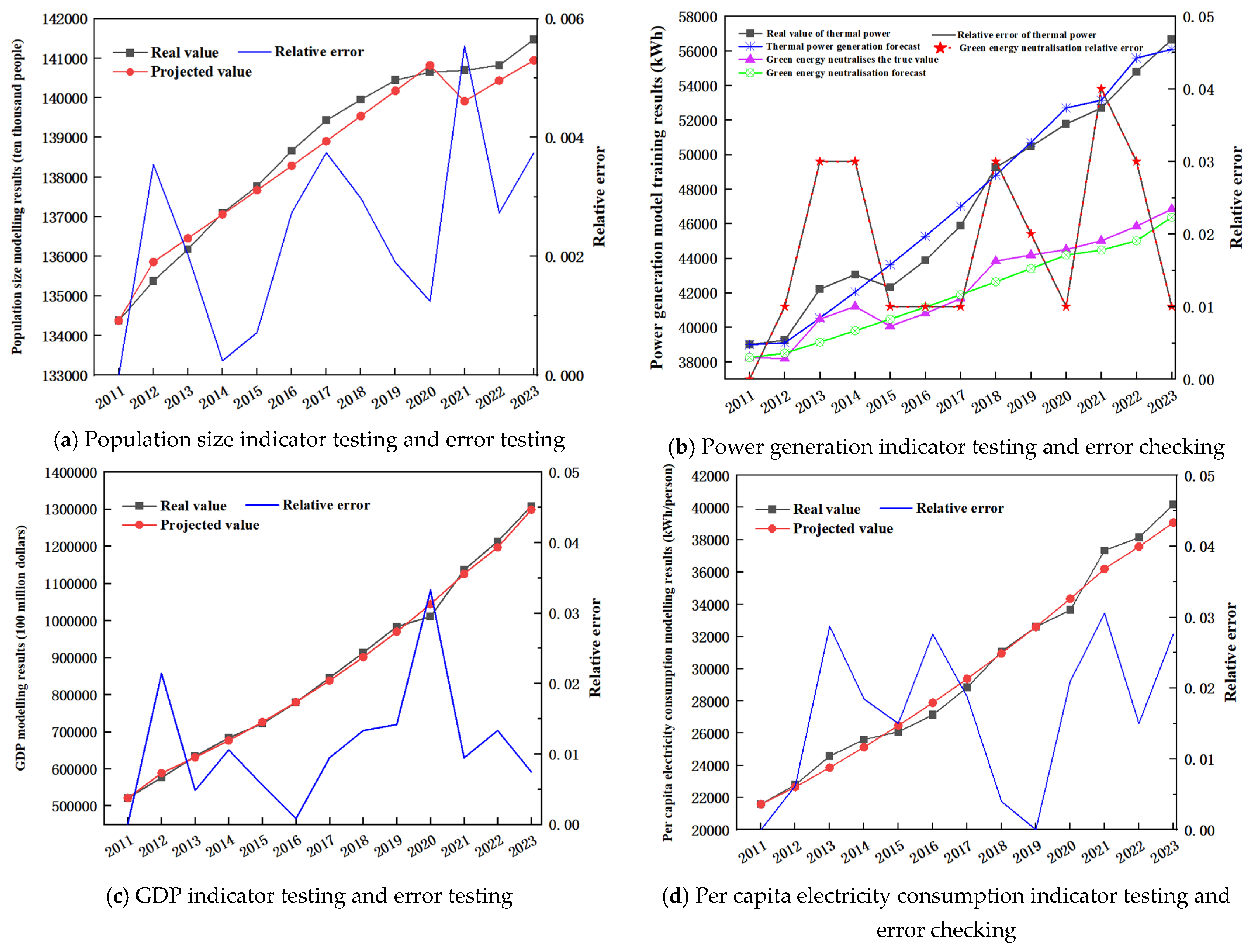
GM(1,1) module accuracy test
Based on the above model analysis, the GM(1,1) model’s training set uses the 2011–2023 real-value indicators as sample data. After testing the model, the predicted values for the 2011–2023 data are obtained. The relative error between the actual and predicted values is within 0.05, indicating good predictive performance. The model’s prediction results are depicted in Figure 6.
2.
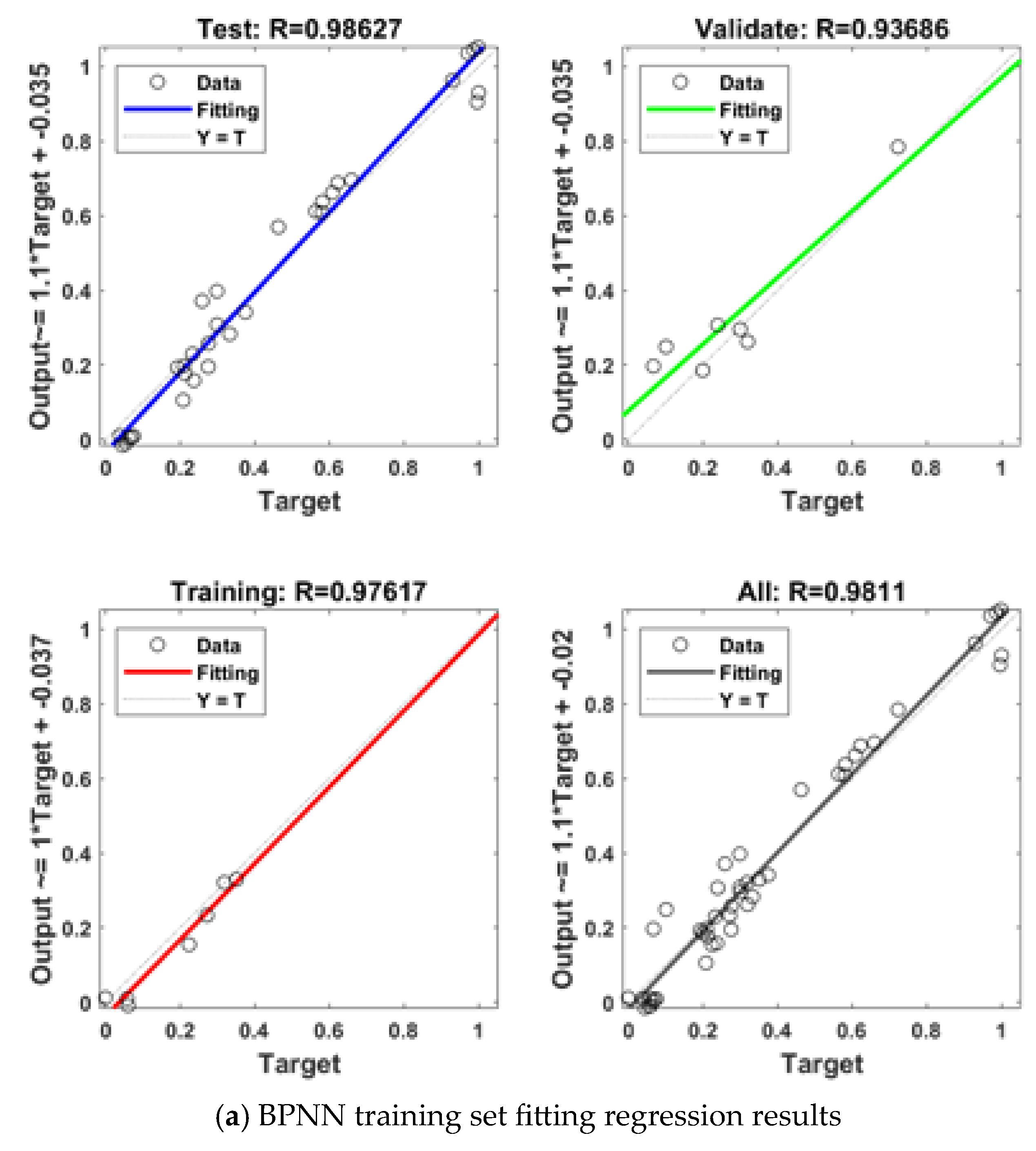
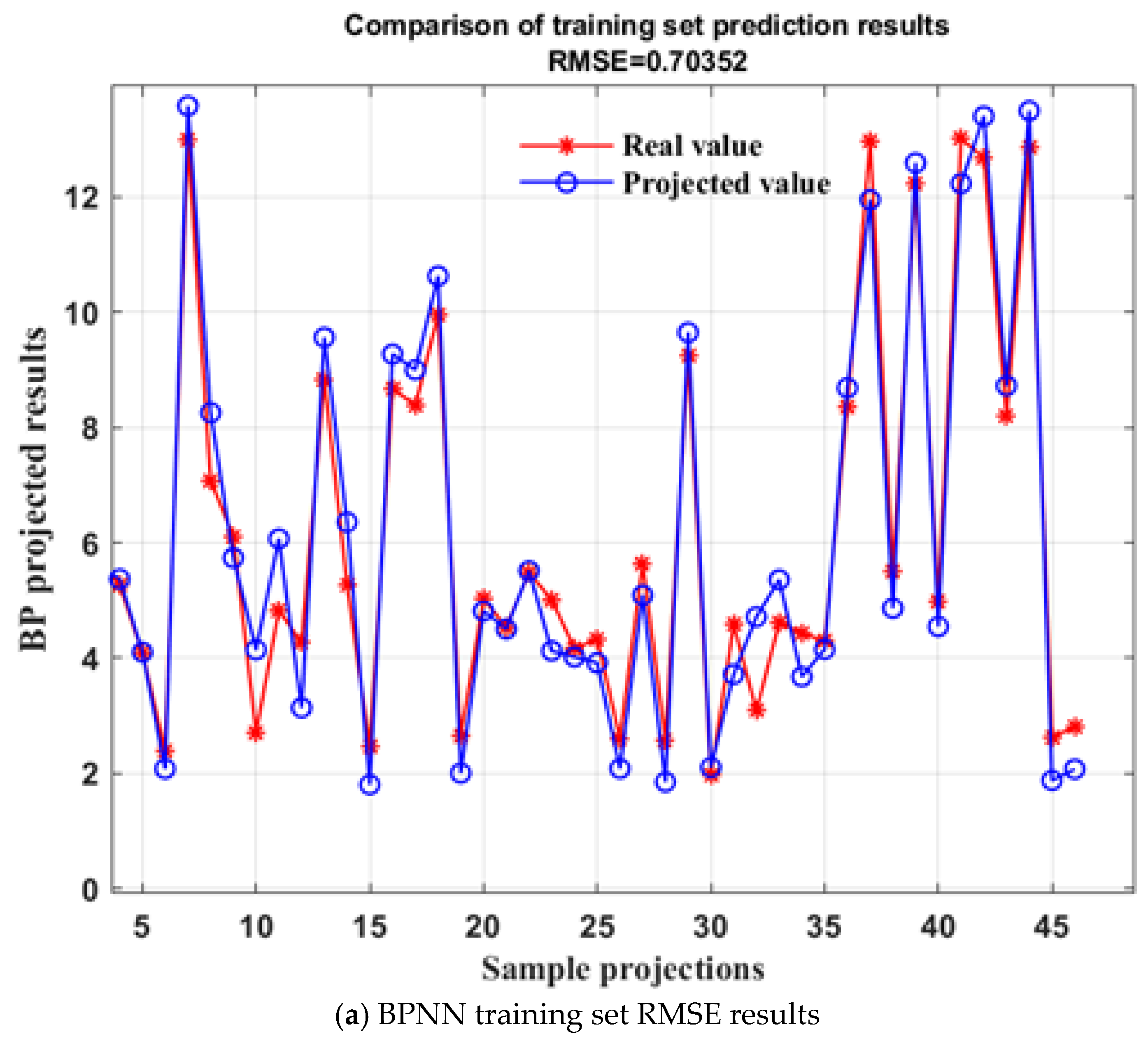
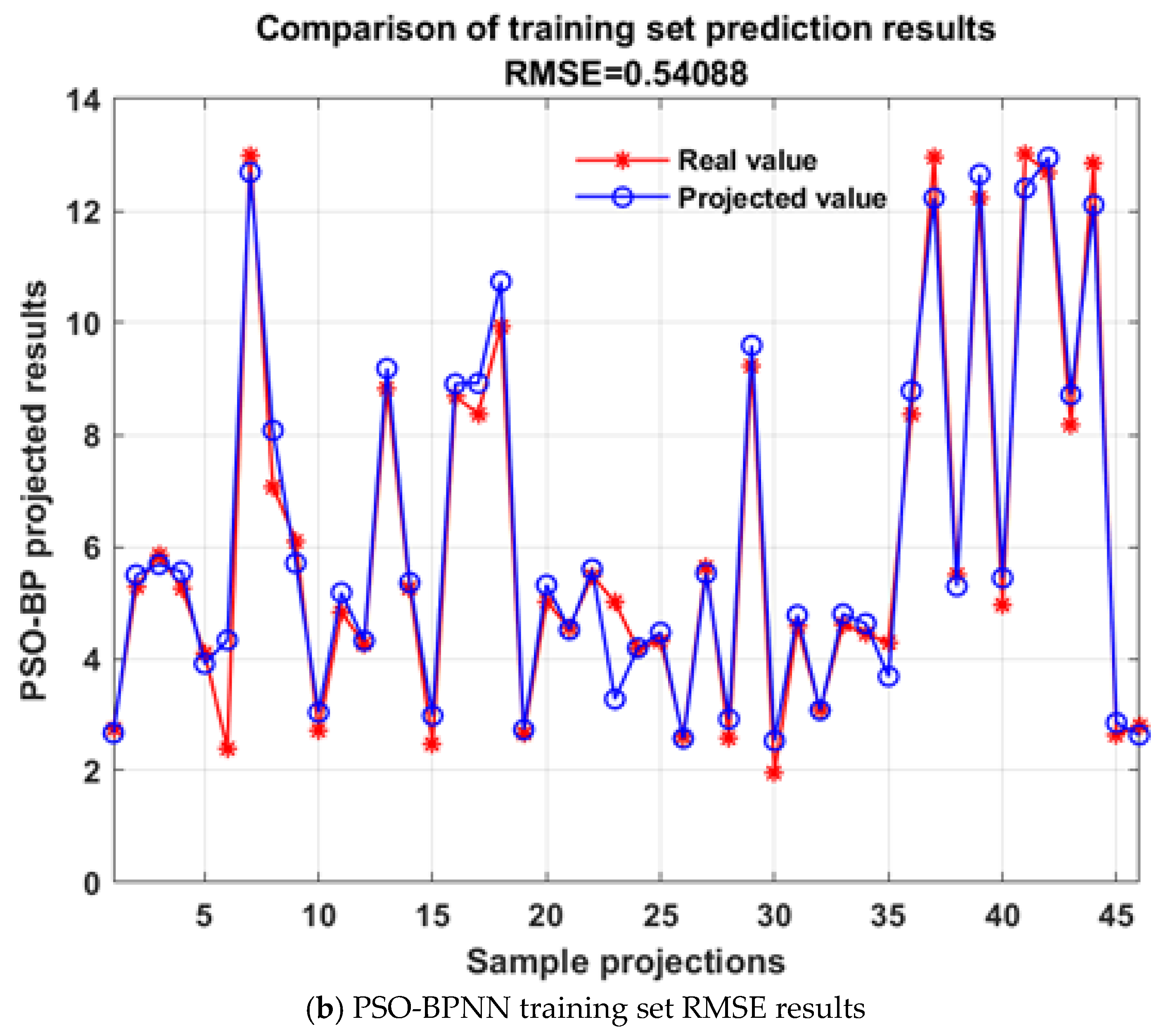
Neural Network Module Accuracy Test
To compare the prediction accuracy of different neural network models, this paper uses four error metrics: MAPE, RMSE, R2, and MAE. MAPE represents the average percentage error per observation, RMSE quantifies the magnitude of the model’s prediction error, R2 indicates how well the model explains the observed variance, and MAE measures the average absolute value of the prediction error. The respective calculation formulas are given below:
M A P E = ( 1 / n ) i = 1 n ( y i y ^ i ) / y i × 100 %
R M S E = ( 1 / n ) i = 1 n ( y i y ^ i ) 2
R 2 = 1 ( i = 1 n ( y i y ^ i ) 2 / i = 1 n ( y i y ¯ i ) 2
M A E = ( 1 / n ) i = 1 n y i y ^ i
where n denotes the total amount of samples of the prediction model; y ^ i , y i and y ¯ i   are the predicted value of the i the sample point, the real true value, and the mean of all samples, respectively.
The neural network model utilizes the output set of the GM(1,1) model as the input layer of the BP network, while the carbon emissions of the power industry influenced by green energy serve as the output layer. The input layer of a neural network is composed of 4 neurons, the hidden layer has 8 neurons, and the output layer consists of 1 neuron. The Levenberg-Marquardt algorithm is chosen for its superior convergence during the training procedure of BPNN. The BPNN is configured with a learning rate of 0.1 and an accuracy rate of 0.0001, using 1000 samples. The dataset Is randomly divided into the training and test sets, with 120 samples in the training set and 66 samples in the test set.
As depicted in Table 2, the comparison of prediction errors among different network models in estimating carbon emissions reveals that the PSO-BPNN attains superior prediction accuracy compared to the BP neural network. The RMSE, MAE, and MAPE of PSO-BPNN are 0.37166, 0.23043, and 0.052377, which are smaller than the corresponding metrics for the BP neural network. Figure 7 and Figure 8 demonstrate that when both the PSO-BPNN and BPNN are utilized for predicting carbon emissions in the power industry, the agreement between the predicted and actual values is strong, with the PSO-BPNN achieving a higher level of agreement than the traditional BP model, reaching 0.99368.
In an attempt to increase the prediction accuracy of CO2 emissions in the power industry, the GM(1,1) model is integrated with the PSO-BPNN, which delivers the highest level of precision. Figure 9 and Table 3 display the comparison between forecasted and actual values of carbon emissions using individual prediction models and combined prediction models. The findings reveal that the combined model has a significantly smaller prediction error than the individual model, with an identification accuracy of 99.46%, outperforming that of the individual model. Therefore, the GM(1,1)-PSO-BPNN hybridized model offers a dependable approach to predicting CO2 emissions in the power system.

4. Result and Discussion

4.1. Projected Result Analysis

In the interest of studying the current status of carbon quota allocation to regional power grids under the carbon peaking target, this paper takes 2030 as the study year, and the initial carbon emission quotas of its six power grids are mainly distributed in three interval bands, which are 0–1 million tons, 5–10 million tons, and 10–15 million tons.

4.1.1. Projected Results of Indicators

On the basis of the GM(1,1) model for China’s 2024–2030 power industry carbon emission impact indicators prediction (the predicted results are shown in Table 4), it was found that in 2030 China’s power generation reached 53,707.9 kWh, per capita electricity consumption reached 15,051.98 kWh/person, the population growth gradually leveled off to 147,666.8 million people, and the future may reach the state of population saturation, and the GDP value will reach 224,876.3 billion yuan.

4.1.2. Results of Initial Quota Projections

The predicted results according to PSO-BPNN are shown in Figure 10, in 2030, the peak CO2 emission from thermal power generation in China’s power industry will reach 5644.54 million tons. After accounting for the neutralization effect of green energy, CO2 emissions will be decreased to 5511.46 million tons, with green energy generation offsetting 133 million tons of emissions. Since this paper primarily studies the effect of green energy production on carbon emissions in the power industry, it examines only the CO2 emissions of regional power grids after taking into account the influence of green energy. Among these, the North China power grid is expected to emit 1376.31 million tons, ranking first, followed by the Northwest power grid at approximately 1106.09 million tons, while the Northeast power grid will have the lowest emissions, with only 334.06 million tons.

4.2. Carbon Allowance Reallocation Results

Given the complexity of the power structure in China, the electric power system should allocate CO2 emission allowances on the basis of the actual conditions of regional power production and electricity consumption to minimize the phenomenon of “carbon transfer”. The core issue, under the shared responsibility principle, is how to determine carbon emissions’ shared proportions among provinces. In the absence of detailed data on energy consumption by provincial power grids and inter-provincial or regional electricity transfers, the actual production-side ratio is used as a proxy for the shared responsibility coefficient, considering the interaction between economic output and electricity load.
θ i = 0.35 ( 1 k i ) / P e c i + 0.65 s i
In the formula, θ i   represents the actual production-side ratio (i.e., the emission reduction responsibility coefficient), ki denotes the power generation efficiency in the region, and s i represents the electricity consumption efficiency in the region. P e c i refers to the per capita electricity consumption (kWh/person) in region iii. The calculations for k i and s i   are provided in the following formulas.
k i = E C V / G e i
s i = G D P i / E c i
ECV represents the power equivalent value of 0.1229 kgce/kWh, G e i   denotes the green and post-generation (10,000 kWh), and E c i represents the electricity consumption in region i (100 million kWh). The shared responsibility coefficient   θ i for each regional power grid is determined by calculating the values of k i and s i , with the results presented in Table 5.
Therefore, on the premise that the overall carbon peak volume limits in the national power system remain unchanged, considering and avoiding the risk of “carbon transfer”, the actual carbon dioxide emission of each regional power grid E P i is as follows:
E P i = θ i · E M g 2030 i
Among them, E M g 2030 i represents the value of green energy and CO2 emissions in year. The actual CO2 quota allocation results of each regional power grid in 2025–2030 are presented in Table 6, and the comparison results of the initial CO2 emissions of each region and the actual carbon quota are presented in Figure 11 and Table 7.
Based on the above model building and the final carbon quota allocation measurement, the initial carbon quota for each regional grid is determined by the total carbon quota in 2030 and the corresponding shared emission reduction responsibility coefficient for each region. Based on the prediction of the total amount of carbon quota for the power industry in the previous section, this paper uses the predicted carbon emission value after the neutralization of green energy power generation as the total amount of carbon quota for the allocation of carbon quota for each regional power grid. According to the above table of shared emission reduction responsibility coefficients of each region, the initial carbon quota allocation results of each region in 2025–2030 are calculated. In order to study the current status of carbon quota allocation of each regional power grid under the carbon peak target, this paper takes 2030 as the study year, and the initial carbon emission quotas of its six power grids are mainly distributed in three interval bands, which are 0–1 billion tons, 5–1 billion tons, and 1–1.5 billion tons.
Among them, the Northeast Power Grid, located in the east of China, has the smallest initial carbon emission quota, receiving only 194.146 million tons of carbon quota, which is mainly because the Northeast region accounts for a large proportion of thermal power generation (the proportion of thermal power generation is more than 90%), and its population and economic development level are in a negative growth trend, so the level of emission reduction potential is low, and therefore it receives a smaller share of carbon emission quota. The initial carbon emission quotas for the North China Power Grid and the Northwest Power Grid are between 500 million and 1 billion tons. The region has a balanced share of thermal power generation and green power generation (each accounting for 50%), and the regional population and economic development level continue to grow, i.e., the emission reduction capacity and potential are higher, so the power sectors in these regions are allocated 873,286, and 522,694 million tons of initial carbon emission quotas, respectively. The remaining two have initial carbon emission quotas of between 1.0 and 1.5 billion tons, and East China, Central China, and the Southern Power Grid show a rapid growth trend in their green power generation technologies and economic development levels in the next five years and therefore have higher emission reduction potentials and receive more carbon emission quotas. The results of the initial allocation of carbon allowances to the power sector show that there are large differences between the initial carbon allowances of the power sector in different regions.

5. Conclusions

This paper, based on the implementation of national grid construction and emission reduction efforts, establishes a reasonable carbon quota allocation scheme within the top-level design framework of the carbon trading market. It employs the GM(1,1)-PSO-BPNN hybridized model to determine total carbon quota allocation for the power industry and uses the shared responsibility coefficient for emission reduction. Based on the total measurement results and assuming the total carbon emissions remain unchanged by 2030, the model redistributes carbon emissions among regional power grids. The detailed conclusions are drawn as follows:
1.
The PSO algorithm is integrated into the traditional BP neural network to perform a global optimization search for the initial weights and thresholds. This approach successfully helps the BP neural network escape local extrema. The performance metrics of the PSO-BPNN optimization algorithm are significantly higher than those of the traditional BP algorithm, and its overall fit surpasses that of other algorithms.
2.
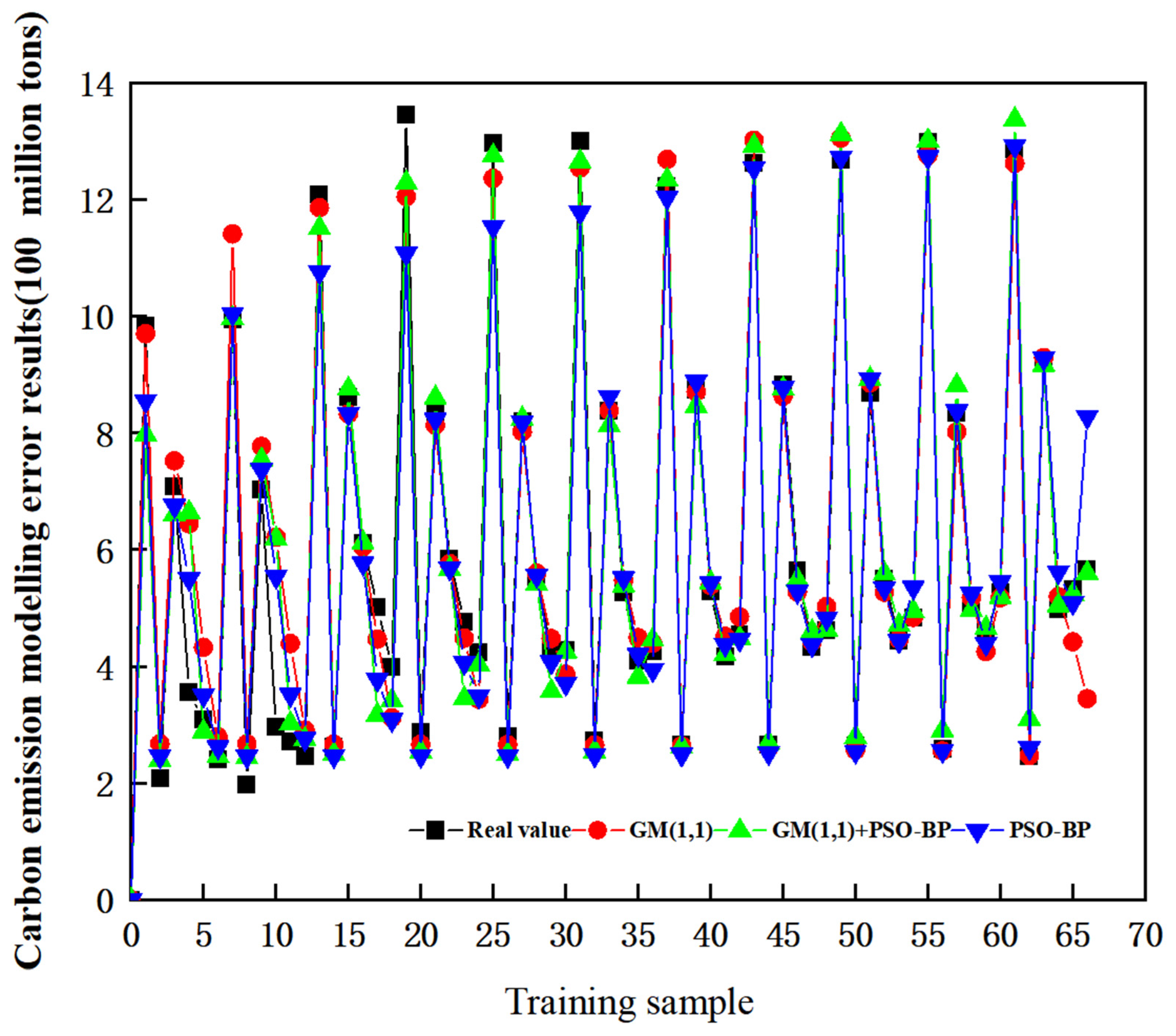
Given that carbon emissions are influenced by multiple factors, such as regional economic development, power structure, and technology level, rather than a single factor, the GM(1,1) algorithm is incorporated into the neural network. Testing revealed that the GM(1,1)-PSO-BPNN hybridized model achieves a prediction accuracy of 99.07% for CO2 emissions in the power industry, significantly surpassing the accuracy of single learning algorithms. Thus, the combined model can be effectively used as a carbon emission prediction tool for the power sector.
3.
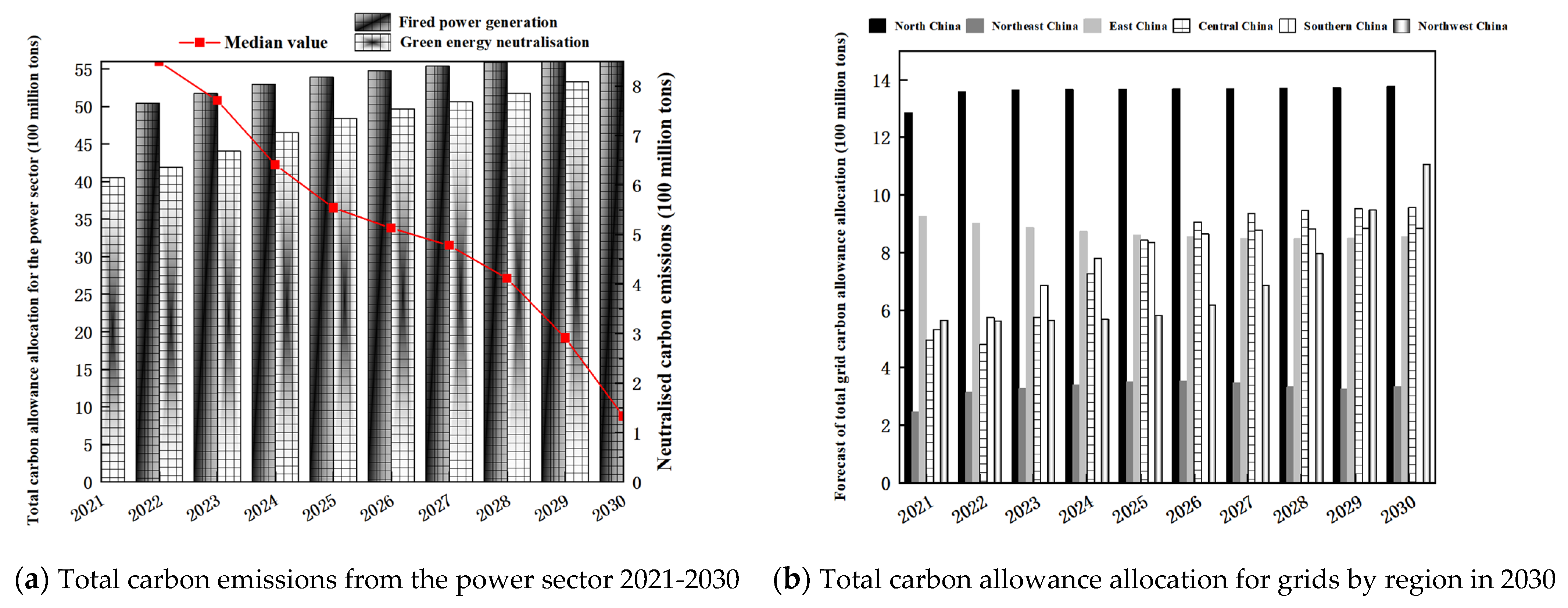
Based on the projections of the combined model, all four quantitative indicators related to carbon emissions are expected to show an upward trend from 2024 to 2030. While China’s power generation, per capita electricity consumption, and GDP are growing rapidly, population growth is slowing and gradually approaching saturation. The study on the influence of green energy on CO2 emissions indicates that China’s power sector can reduce its peak carbon emissions in 2030 by 133 million tons, lowering them to 5511.46 million tons during and after green energy generation.
4.
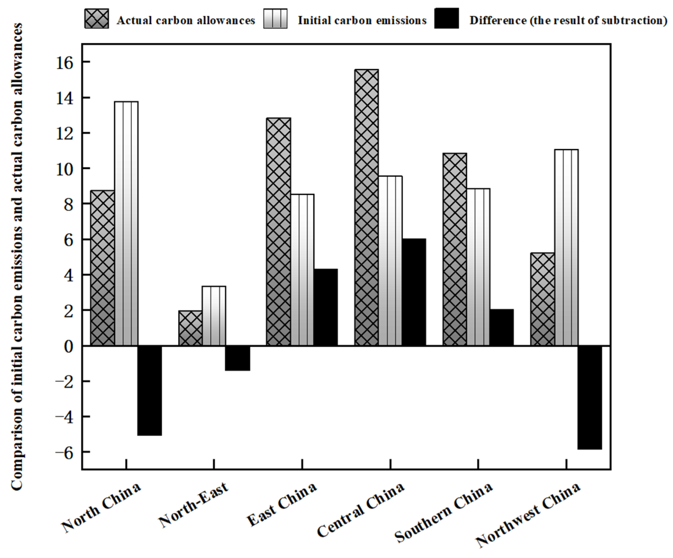
Due to the complexity and variability of the internal structure of the power system, it is challenging for government departments to delineate the actual emission reduction responsibilities between power-generating and power-using regions. Therefore, shared responsibility coefficients are adopted to mitigate the risk of “carbon transfer” and to determine the actual emission reduction responsibility coefficients for each regional power grid. Based on model development and the adjustment of these responsibility coefficients, this paper proposes a fair and reasonable carbon quota allocated program for the power sector.

6. Research Shortcomings and Prospects

There are some research limitations in this study, as follows:
1.
As this study adopts the GM(1,1) model to predict the carbon emission-related indicators of the electric power industry, the model itself adopts the exponential function growth, which grows too fast, leading to further research on whether the related indicators can reach that growth rate in the future.
2.
In the carbon emissions measurement, taking into account the impact of green energy, due to regional differences, the adoption of green energy power generation technology level is limited in each region, making it difficult to obtain energy neutralization data, and has certain limitations in analyzing the impact of green energy on regional carbon emissions.

Author Contributions

Conceptualization, Y.S. and Y.X.; methodology, Y.X.; software, Y.X. and Z.Z.; validation, Y.T. and S.L.; formal analysis, Y.X. and S.L.; resources, Y.X. and Y.S.; data curation, Y.T. and S.L.; writing—original draft preparation, Y.X.; writing—review and editing, S.J., Z.Z. and Y.Y.; visualization, S.J. and Z.Z.; supervision, Y.S. and Y.T.; project administration, Y.S., S.J. and Y.Y.; funding acquisition, Y.S. and Y.Y. All authors have read and agreed to the published version of the manuscript.

Funding

This research was funded by the National Natural Science Foundation of China (42201293, 42101260) and the Social Science Planning Fund of Liaoning Province (L24AWT012).

Institutional Review Board Statement

Not applicable.

Informed Consent Statement

Not applicable.

Data Availability Statement

The raw data supporting the conclusions of this article will be made available by the authors on request.

Conflicts of Interest

The authors declare no conflicts of interest. The funders had no role in the design of the study; in the collection, analyses, or interpretation of data; in the writing of the manuscript; or in the decision to publish the results.

References

  1. Daaboul, J.; Moriarty, P.; Honnery, D. Net green energy potential of solar photovoltaic and wind energy generation systems. J. Clean. Prod. 2023, 415, 137806. [Google Scholar] [CrossRef]
  2. Buestán-Andrade, P.A.; Peñacoba-Yagüe, M.; Sierra-García, J.E.; Santos, M. Wind Power Forecasting with Machine Learning Algorithms in Low-Cost Devices. Electronics 2024, 13, 1541. [Google Scholar] [CrossRef]
  3. Wang, M.; Zhou, P. Impact of Permit Allocation on Cap-and-trade System Performance under Market Power. Energy J. 2020, 41, 215–231. [Google Scholar] [CrossRef]
  4. Bai, M.R.; Li, C.B. Research on the allocation scheme of carbon emission allowances for China’s provincial power grids. Energy 2024, 299, 131551. [Google Scholar] [CrossRef]
  5. Groh, E.; Ziegler, A. On self-interested preferences for burden sharing rules: An econometric analysis for the costs of energy policy measures. Energy Econ. 2018, 74, 417–426. [Google Scholar] [CrossRef]
  6. Rose, A. Reducing conflict in global warming policy-the potential of equity as a unifying principle. Energy Policy 1990, 18, 927–935. [Google Scholar] [CrossRef]
  7. Pozo, C.; Galán-Martín, Á.; Reiner, D.M.; Mac Dowell, N.; Guillén-Gosálbez, G. Equity in allocating carbon dioxide removal quotas. Nat. Clim. Chang. 2020, 10, 640–646. [Google Scholar] [CrossRef]
  8. Tian, Y.; Chen, C. China’s Provincial Carbon Emission Reduction Reward and Punishment Programme Based on Carbon Emission Right Allocation. Chin. J. Popul. Resour. 2020, 30, 54–62. [Google Scholar]
  9. Jiang, M.X.; Zhu, B.Z.; Chevallier, J.; Xie, R. Allocating provincial CO2 quotas for the Chinese national carbon program. Aust. J. Agr. Resour. Ec. 2018, 62, 457–479. [Google Scholar] [CrossRef]
  10. Cai, W.G.; Ye, P.Y. A more scientific allocation scheme of carbon dioxide emissions allowances: The case from China. J. Clean. Prod. 2019, 215, 903–912. [Google Scholar] [CrossRef]
  11. Fang, M.Y.; Tan, K.S.; Wirjanto, T. Valuation of carbon emission allowance options under an open trading phase. Energy Econ. 2024, 131, 107351. [Google Scholar] [CrossRef]
  12. Li, J.J.; Tian, Y.J.; Zhang, Y.L.; Xie, K.C. Assessing spatially multistage carbon transfer in the life cycle of energy with a novel multi-flow and multi-node model: A case of China’s coal-to-electricity chain. J. Clean. Prod. 2022, 339, 130699. [Google Scholar] [CrossRef]
  13. Li, Y.W.; Yang, X.X.; Du, E.S.; Liu, Y.L.; Zhang, S.X.; Yang, C.; Zhang, N.; Liu, C. A review on carbon emission accounting approaches for the electricity power industry. Appl. Energy 2024, 359, 122681. [Google Scholar] [CrossRef]
  14. Von, W.G.; Cullenward, D.; Mastrandrea, M.D.; Weyant, J. Accounting for the greenhouse gas emission intensity of regional electricity transfers. Environ. Sci. Technol. 2021, 55, 6571–6579. [Google Scholar]
  15. Qu, S.; Li, Y.; Liang, S.; Yuan, J.H.; Xu, M. Virtual CO2 emission flows in the global electricity trade network. Environ. Sci. Technol. 2018, 52, 6666–6675. [Google Scholar] [CrossRef] [PubMed]
  16. Zhang, P.F.; Cai, W.Q.; Yao, M.T.; Wang, Z.Y.; Yang, L.Z.; Wei, W.D. Urban carbon emissions associated with electricity consumption in Beijing and the driving factors. Appl. Energy. 2020, 275, 115425. [Google Scholar] [CrossRef]
  17. Wei, W.D.; Zhang, P.F.; Yao, M.T.; Xue, M.; Miao, J.W.; Liu, B.; Wang, F. Multi-scope electricity-related carbon emissions accounting: A case study of Shanghai. J. Clean. Prod. 2020, 252, 119789. [Google Scholar] [CrossRef]
  18. Li, W.B.; Long, R.; Zhang, L.L.; He, Z.X.; Chen, F.Y.; Chen, H. Greenhouse Gas Emission Transfer of Inter-Provincial Electricity Trade in China. Int. J. Environ. Res. Public Health 2020, 17, 8375. [Google Scholar] [CrossRef] [PubMed]
  19. Eberle, A.L.; Heath, G. Estimating carbon dioxide emissions from electricity generation in the United States: How sectoral allocation may shift as the grid modernizes. Energy Policy 2020, 140, 111324. [Google Scholar] [CrossRef]
  20. Lopez, N.S.; Biona, J.B.M.; Chiu, A.F. Electricity trading and its effects on global carbon emissions: A decomposition analysis study. J. Clean. Prod. 2018, 195, 532–539. [Google Scholar] [CrossRef]
  21. Li, F.Y.; Xiao, X.L.; Xie, W.; Ma, D.W.; Song, Z.; Liu, K.P. Estimating air pollution transfer by interprovincial electricity transsions: The case study of the Yangtze River Delta Region of China. J. Clean. Prod. 2018, 183, 56–66. [Google Scholar] [CrossRef]
  22. Ehigiamusoe, K.U. A disaggregated approach to analyzing the effect of electricity on carbon emissions: Evidence from African countries. Energy Rep. 2020, 6, 1286–1296. [Google Scholar] [CrossRef]
  23. Xu, G.Q.; Feng, S.W. Spatial-temporal evolution characteristics of carbon emissions from energy consumption in China’s thermal power industry. Ecol. Econ. 2024, 40, 30–38. [Google Scholar]
  24. Wang, X.P.; Peng, W.K.; Lu, H.Y.; Yan, F. Forecast of cold chain logistics demand for agricultural products in Beijing based on neural network. GDAAS 2018, 45, 120–128. [Google Scholar]
  25. Zuo, Z.; Niu, Y.; Li, J.; Fu, H.; Zhou, M. Machine Learning for Advanced Emission Monitoring and Reduction Strategies in Fossil Fuel Power Plants. Appl. Sci. 2024, 14, 8442. [Google Scholar] [CrossRef]
  26. Jin, Y.K.; Sharifi, A.; Li, Z.S.; Chen, S.R.; Zeng, S.Z.; Zhao, S.L. Carbon emission prediction models: A review. Sci. Total. Environ. 2024, 927, 172319. [Google Scholar] [CrossRef] [PubMed]
  27. Wang, M.X. Predicting China’s Energy Consumption and CO2 Emissions by Employing a Novel Grey Model. Energies 2024, 17, 5256. [Google Scholar] [CrossRef]
  28. Zhao, Z.H.; Zhang, X.H.; Wang, T.; Liu, K.; Zhang, L.M. Predicting of carbon emission in the power industry based on the RFR model optimized by EABC algorithm. Shandong Electr. Power. 2024, 51, 77–84. [Google Scholar]
  29. Li, H.B.; Zhang, J.J. A new model for natural gas demand forecasting and its application—Takes Sichuan-Chongqing region as an example. Nat. Gas. Ind. 2021, 41, 935–951. [Google Scholar]
  30. He, X.; Wen, Y.; Zhang, D. A Fast Prediction Method for the Electromagnetic Response of the LTE-R System Based on a PSO-BP Cascade Neural Network Model. Appl. Sci. 2023, 13, 6640. [Google Scholar] [CrossRef]
  31. Mulumba, D.M.; Liu, J.; Hao, J.; Zheng, Y.; Liu, H. Application of an Optimized PSO-BP Neural Network to the Assessment and Prediction of Underground Coal Mine Safety Risk Factors. Appl. Sci. 2023, 13, 5317. [Google Scholar] [CrossRef]
  32. Hu, Y.C. Electricity Consumption Prediction Using a Neural-Network-Based Grey Forecasting Approach. J. Oper. Res. Soc. 2017, 68, 1259–1264. [Google Scholar] [CrossRef]
  33. Chiang, C.C.; Ho, M.C.; Chen, J.A. A Prediction Model for Shallow Groundwater Level in Harbin Based on GA-PSO-BP. Neural Comput. Appl. 2006, 15, 328–338. [Google Scholar] [CrossRef]
  34. Wang, X.L.; Dai, C.L.; Wen, J.W.; Qi, Y.; Zhang, Q.S. Shallow ground water level prediction model in Harbin city based on GA-PSO-BP. J. Zhejiang Univ. Water Resour. Hydropower Eng. 2023, 35, 27–31. [Google Scholar]
  35. Liu, H.J.; Shao, H.B. Research on prediction of aerospace panel clamping deformation based on SSA-PSO-BP neural network. Mach. Tool. Hydraul. 2023, 51, 114–120. [Google Scholar]
  36. Zheng, L.H.; Sun, Y.L.; Yu, Y. Carbon Peak Control Strategies and Pathway Selection in Dalian City: A Hybrid Approach with STIRPAT and GA-BP Neural Networks. Sustainability 2024, 16, 8657. [Google Scholar] [CrossRef]
  37. Yang, J.; Zhang, X.; Liu, S.; Yang, X.; Li, S. Rolling Bearing Residual Useful Life Prediction Model Based on the Particle Swarm Optimization—Optimized Fusion of Convolutional Neural Network and Bidirectional Long–Short-Term Memory–Multihead Self-Attention. Electronics 2024, 13, 2120. [Google Scholar] [CrossRef]
  38. Ellahi, M.; Usman, M.R.; Arif, W.; Usman, H.F.; Khan, W.A.; Satrya, G.B.; Daniel, K.; Shabbir, N. Forecasting of Wind Speed and Power through FFNN and CFNN Using HPSOBA and MHPSO-BAACs Techniques. Electronics 2022, 11, 4193. [Google Scholar] [CrossRef]
  39. Zhang, X.L.; Liu, X.Q.; Zhang, Z.Y.; Tang, R.Y.; Zhang, T.; Yao, J. The Synergistic Effect of the Carbon Emission Trading Scheme on Pollution and Carbon Reduction in China’s Power Industry. Sustainability 2024, 16, 8681. [Google Scholar] [CrossRef]
  40. Jin, J.L.; Zhang, X.Y.; Xu, L.L.; Wen, Q.L.; Guo, X.J. Impacts of carbon trading and wind power integration on carbon emission in the power dispatching process. Energy Rep. 2021, 7, 3887–3897. [Google Scholar] [CrossRef]
  41. Wang, B.J.; Zhao, J.L.; Wei, Y.X. Carbon emission quota allocating on coal and electric power enterprises under carbon trading pilot in China: Mathematical formulation and solution technique. J. Clean. Prod. 2019, 239, 118104. [Google Scholar] [CrossRef]
  42. Meng, M.; Wang, L.X.; Chen, Q. Quota Allocation for Carbon Emissions in China’s Electric Power Industry Based Upon the Fairness Principle. Energies 2018, 11, 2256. [Google Scholar] [CrossRef]
  43. Wang, Y.Q.; Qiu, J.; Tao, Y.C.; Zhao, J.H. Carbon—Oriented Operational Planning in Coupled Electricity and Emission Trading Markets. IEEE Trans. Power Syst. 2020, 35, 3145–3157. [Google Scholar] [CrossRef]
  44. Ma, C.Q.; Ren, Y.S.; Zhang, Y.J.; Sharp, B. The allocation of carbon emission quotas to five major power generation corporations in China. J. Clean. Prod. 2018, 189, 1–12. [Google Scholar] [CrossRef]
  45. Zhang, L.R.; Li, Y.K.; Jia, Z.J. Impact of carbon allowance allocation on power industry in China’s carbon trading market:Computable general equilibrium based analysis. Appl. Energy 2018, 229, 814–827. [Google Scholar] [CrossRef]
  46. Lyu, W.R.; Cui, Z.G.; Yuan, M.; Shan, E.F. Cooperation for trans-regional electricity trading from the perspective of carbon quota: A cooperative game approach. Int. J. Electr. Power. Energy Syst. 2024, 156, 109773. [Google Scholar] [CrossRef]
  47. Zhu, Q.Y.; Chen, X.F.; Song, M.L.; Li, X.C.; Shen, Z.Y. Impacts of renewable electricity standard and Renewable Energy Certificates on renewable energy investments and carbon emissions. J. Environ. Manag. 2022, 306, 114495. [Google Scholar] [CrossRef]
  48. Li, J.G.; Mao, T.; Huang, G.L.; Zhao, W.M.; Wang, T. Research on Day-Ahead Optimal Scheduling Considering Carbon Emission Allowance and Carbon Trading. Sustainability 2023, 15, 6108. [Google Scholar] [CrossRef]
  49. Wang, Y.X.; Huang, H.Q.; Chen, Y.; Dong, M.Q.; Li, S.W.; Yue, S.J.; Lu, Z.W. Analysis of carbon emission drivers in Chinese power consumption— Based on LMDI decomposition method. J. Hubei Univ. Econ. 2023, 20, 38–44. [Google Scholar]
  50. Wei, Y.M.; Wang, X.Y.; Ding, Y.H.; Zheng, J.; Shan, Z.J. Provincial carbon quota allocation for China’s electric power industry considering carbon transfer under the carbon peaking target. J. Arid. Land 2023, 37, 19–26. [Google Scholar]
  51. Tang, T.; Jiang, W.H.; Zhang, H.; Nie, J.T.; Xiong, Z.H.; Wu, X.G.; Feng, W.J. GM (1,1) based improved seasonal index model for monthly electricity consumption forecasting. Energy 2022, 252, 124041. [Google Scholar] [CrossRef]
  52. Rumelhart, D.; Hinton, G.; Williams, R. Learning representations by back-propagating errors. Nature 1986, 323, 533–536. [Google Scholar] [CrossRef]
  53. Wang, L.; Yi, S.; Yu, Y.; Gao, C.; Samali, B. Automated ultrasonic-based diagnosis of concrete compressive damage amidst temperature variations utilizing deep learning. Mech. Syst. Signal Process 2024, 221, 111719. [Google Scholar] [CrossRef]
  54. Yu, Y.; Zhang, C.; Xie, X.; Yousefi, A.M.; Zhang, G.; Li, J.; Samali, B. Compressive strength evaluation of cement-based materials in sulphate environment using optimized deep learning technology. Dev. Built Environ. 2023, 16, 100298. [Google Scholar] [CrossRef]
  55. Yu, Y.; Rashidi, M.; Dorafshan, S.; Samali, B.; Farsangi, E.N.; Yi, S.; Ding, Z. Ground penetrating radar-based automated defect identification of bridge decks: A hybrid approach. J. Civ. Struct. Health. Monit. 2024. [Google Scholar] [CrossRef]
Figure 1. Carbon emissions trends, 2011–2023.
Applsci 14 11996 g001
Figure 2. Trends in carbon emission-related features.
Applsci 14 11996 g002
Figure 3. GM(1,1) + BP combined prediction model.
Applsci 14 11996 g003
Figure 4. BP neural network algorithm.
Applsci 14 11996 g004
Figure 6. GM(1,1) Module Training Results.
Applsci 14 11996 g006
Figure 7. Results of BPNN and PSO-BPNN model fitting.
Applsci 14 11996 g007aApplsci 14 11996 g007b
Figure 8. BPNN and PSO-BPNN model training results.
Applsci 14 11996 g008aApplsci 14 11996 g008b
Figure 9. Combined model with a single model.
Applsci 14 11996 g009
Figure 10. Results of carbon allowance projections.
Applsci 14 11996 g010
Figure 11. Comparison of redistribution with initial quota.
Applsci 14 11996 g011
Table 1. Carbon emission evaluation indicator system.
First-Level IndicatorsSecond-Level Indicators
Emission reduction responsibilityPower generation (thermal power generation,
Green energy neutralized power generation)
Emission reductionPotential population
Per capita electricity consumption
Emission reduction capacityGDP
Table 2. Neural network model performance evaluation.
Training SetBPNNPSO-BPNN
RMSE0.703520.54088
MAE0.596630.38247
MAPE0.131580.08125
R20.953880.97274
Table 3. Error between predicted and real values.
ModelGM(1,1)PSO-BPGM(1,1) + PSO-BP
Average Error0.107130530.096732090.08855026
Accuracy Rate0.987340.993680.99457
Table 4. Carbon emission indicator projection results.
YearPopulation NumberGDPThermal Power Generation CapacityPost-Neutralization Power GenerationElectricity Consumption per Capita
2024143,472.81,411,31261,713.947,617.0310,369.60
2025144,153.11,523,63164,268.048,546.8411,033.36
2026144,840.71,645,63266,957.049,508.2011,740.30
2027145,536.61,778,17869,790.850,505.6112,492.39
2028146,240.81,922,17572,778.851,536.2713,293.03
2029146,950.22,078,68475,930.252,602.2314,145.05
2030147,666.82,248,76379,258.453,707.9015,051.98
Table 5. Coefficient of emission reduction responsibility for regional grids.
YearNorth ChinaNortheast ChinaEast ChinaCentral ChinaSouthern ChinaNorthwest China
20240.674510.713881.212641.344721.031010.45959
20250.667670.689831.256751.388191.061310.46176
20260.660900.666581.302541.433021.092500.46390
20270.654190.644101.349921.479351.124600.46607
20280.647580.622411.399071.527111.157690.46820
20290.641020.601451.449951.576481.191730.47040
20300.634510.581171.502751.627431.226720.47256
Table 6. Results of carbon quota reallocation.
YearNorth ChinaNortheast ChinaEast ChinaCentral ChinaSouthern ChinaNorthwest ChinaNationwide
20259.1262.41910.82211.6988.8642.68845.618
20269.0352.35711.11112.9839.4402.86347.790
20278.9492.23811.45513.8239.8643.19349.520
20288.8692.08211.85814.45310.2143.72851.204
20298.7971.95712.31815.01310.5374.45653.077
20308.7331.94112.83215.56410.8545.22755.151
Table 7. Comparison of initial and final quotas.
AreaActual Carbon Quota
(100 Million Tons)
Forecast Carbon Emissions (100 Million Tons)Difference
(100 Million Tons)
North China8.73313.763−5.030
Northeast China1.9423.341−1.399
East China12.8328.5394.293
Central China15.5649.5646.001
Southern China10.8548.8482.006
Northwest China5.22711.061−5.834
Disclaimer/Publisher’s Note: The statements, opinions and data contained in all publications are solely those of the individual author(s) and contributor(s) and not of MDPI and/or the editor(s). MDPI and/or the editor(s) disclaim responsibility for any injury to people or property resulting from any ideas, methods, instructions or products referred to in the content.

