Autonomous Driving Decision-Making Method Based on Spatial-Temporal Fusion Trajectory Prediction

Abstract

Due to the challenge that the behavior of traffic participants in the driving environment is highly stochastic and uncertain, it is difficult for self-driving vehicles to make accurate decisions based only on the current environmental state. In this paper, we propose a driving strategy learning method based on spatial-temporal feature prediction. Firstly, the spatial interaction between vehicles is implicitly modeled using a graph convolutional neural network and multi-head attention mechanism, and the gated loop unit is embedded to capture the sequential temporal relationship to establish a prediction model incorporating spatial-temporal features. Then, a reinforcement learning-based driving strategy method is constructed using some of the predictive features of the ego-vehicle and surrounding vehicles as predictive state inputs. Finally, based on the real dataset and CARLA simulation platform, the prediction ability of the prediction model and the effectiveness of the prediction-based decision-making model are verified. The simulation results prove that the prediction algorithm can achieve the minimum error compared with the baseline trajectory prediction algorithm, and effectively improves the accuracy and reliability of the autopilot decision-making in various dynamic scenarios.

1. Introduction

Autonomous driving technology is seen as the key to achieving a safer and more efficient transportation future. However, there are still important challenges in realizing reliable and stable autonomous driving technologies. The main problem is that the behavior of traffic participants in the driving environment is random, and the complex interaction between vehicles makes it difficult for autonomous vehicles to accurately identify and predict the behavior of other traffic participants, which in turn affects the ability of vehicles to safely and efficiently make decisions in environments full of ‘uncertainty’.

Traditional decision-making models only rely on the state of the surrounding environment at the current moment [1]. However, with the change of time, the uncertainty of the behavior of traffic participants may lead to a huge error between ego-vehicle decisions and the dynamically changing driving environment. Therefore, reasonable prediction of future driving trajectories of traffic participants in the environment can help to guarantee the efficiency and safety of decision-making effects [2].

In the research of trajectory prediction, recurrent neural networks [3] and graph neural networks [4] are the two more common networks at present. Recurrent neural networks can effectively deal with temporal information and find the pattern between trajectory changes, while graph neural networks can model the interaction relationship between vehicles and improve prediction accuracy [5]. The literature [6] designs a driving intention recognition and vehicle trajectory prediction model based on the Long Short-Term Memory (LSTM) network, and adds a hybrid density network layer to the original encoder-decoder structure to represent the future position of the vehicle using probability distributions, which improves the accuracy of trajectory prediction, but this method is only applicable to conventional scenarios such as highways. The literature [7] enriches the information of traffic participants in the driving scenario expressed by using a graph structure and especially takes features such as pedestrians and obstacles into account for trajectory prediction. The literature [8] proposes a graph-based spatial-temporal convolutional network, which uses a graph convolutional neural network to capture the temporal features and a convolutional neural network to capture the spatial features, and successfully predicts the distribution of future trajectories of neighboring vehicles. However, trajectory prediction is a spatial-temporal task. How to fully utilize these features and improve prediction accuracy remains a key issue.

There are two kinds of existing autonomous driving decision-making methods: rule-based and learning-based [9]. Rule-based methods rely on a large number of manually formulated rules to impose safe and controllable behaviors on the vehicle; however, real environments contain a large number of emergent conditions, and the manual rules often cannot fully cover all working conditions. Learning-based methods rely on a large amount of data for training mainly through neural networks, which can overcome the disadvantage of poor environmental adaptability to a certain extent and have now become the mainstream algorithms for solving the decision-making problem of autonomous driving.

Learning-based methods are primarily categorized into imitation learning (IL) [10] and reinforcement learning (RL) [11]. Imitation learning relies on a large amount of experts’ experience data for learning and lacks the ability to actively explore unseen scenes. On the other hand, reinforcement learning optimizes driving performance through interaction with the environment and repeated trial and error, thus it has stronger scene adaptation and generalization [12]. The literature [13] models self-driving vehicle following scenarios as a classical Markov decision process and solves the optimal following policy for this model using the Q-learning algorithm. The literature [14] proposes a Q-value estimation method based on a weighted average of sample variance, which effectively improves the Q-value underestimation problem of the twin delayed deep deterministic policy gradient (TD3) algorithm. A Deep Deterministic Policy Gradient (DDPG) algorithm considering state distribution is proposed in the literature [15], which guarantees that the reinforcement learning algorithm still has sufficient exploration ability when the scene distribution varies greatly, and is validated in the lane keeping task. The literature [16] used RL to provide informationally supervised signals for IL learning, which greatly improved the success rate of end-to-end intelligent agent decision-making under the ‘guidance’ of RL experts. In [17], to ensure that the optimal performance of the RL model performs optimally in complex traffic scenarios, the sensor input images are preprocessed to reduce the state space while guaranteeing better safety and accuracy of the model.

Comprehensive research has found that most of the current decision-making methods are based on reinforcement learning, in which the state space is equivalent to the “perspective” of the self-driving vehicle, playing a crucial role in the decision-making process. However, most of the existing methods only focus on the current vehicle state and conduct research on general scenarios such as “high speed straight ahead”, “on-ramp convergence”, etc. [18]. Since complex scenarios may not be able to make decisions through conventional methods, it is often too late to react in dynamic scenarios, which leads to limitations in the application of ego-vehicle decision-making capabilities in some complex scenarios. Based on the previous literature, this paper focuses on self-driving vehicle prediction and reinforcement learning decision-making and designs a self-driving decision-making method considering future trajectory prediction through spatial and temporal fusion, aiming to effectively improve decision-making ability under various dynamic driving scenarios.

2. Method

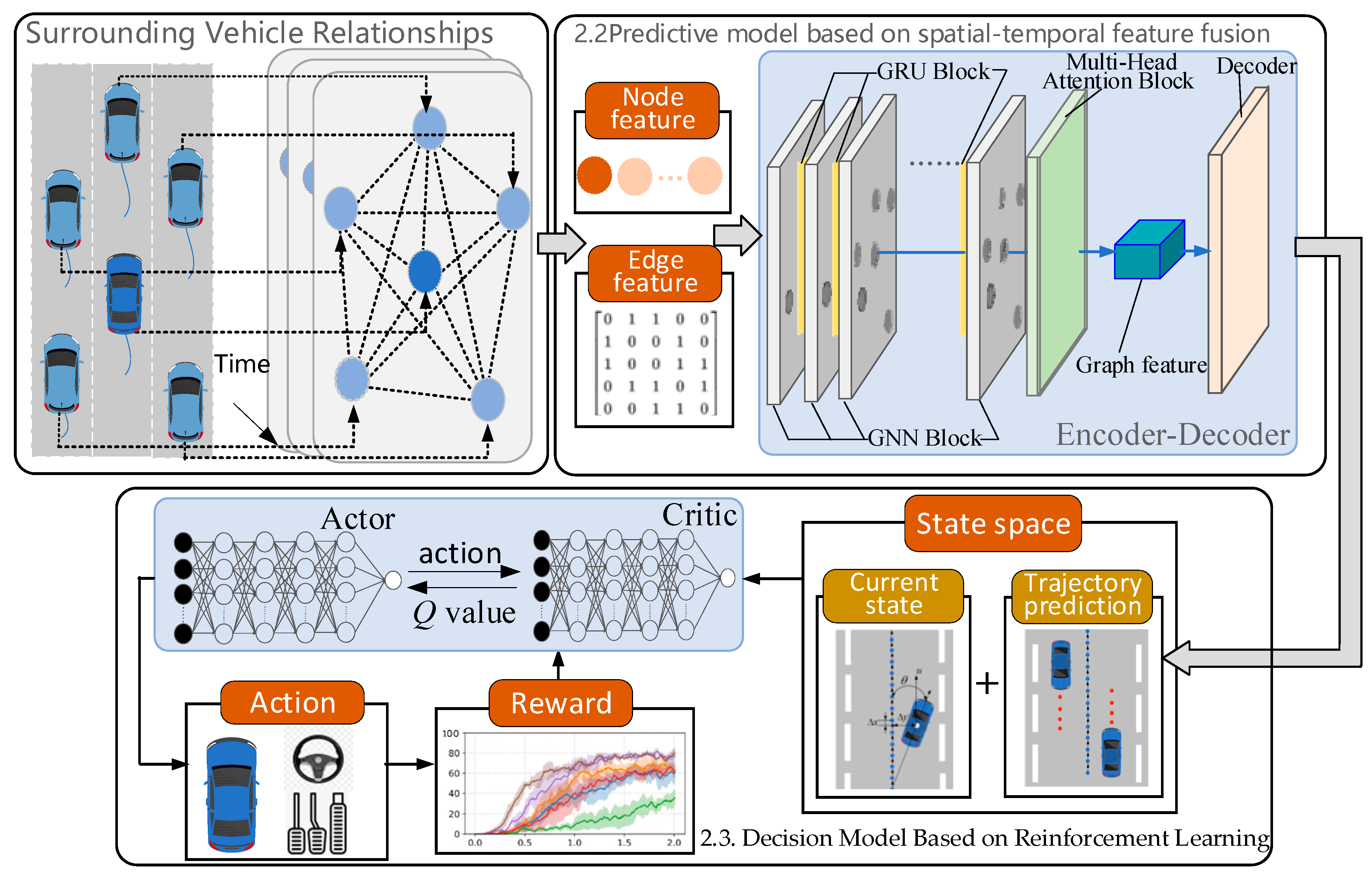
2.1. Overall Structure

The overall structure of the spatial-temporal prediction-based autonomous driving decision-making proposed in this paper is shown in Figure 1. The upper layer architecture of the scheme consists of a trajectory prediction module fusing spatial-temporal features, which delineates vehicles in the range of interest according to the actual traffic scenario, takes the state of the vehicles in the range as the point features and the distance relationship between the vehicles as the edge features, and inputs successive frames of time-series data into the coding module to obtain the graph features, which are decoded based on a decoder to decode the trajectory of the ego-vehicle and the movement of the surrounding vehicles. The lower architecture is a decision model based on the reinforcement learning Soft Actor-Critic (SAC) algorithm [19]. In addition to the current state of the vehicle, its state space also incorporates information about its own and surrounding vehicle trajectories predicted by the upper layer prediction module. The strategy network (Actor) selects the next momentary action based on the current state, while the value network (Critic) evaluates the state value with the action value. Eventually, through the correct guidance of the reward function, the network is able to output reasonably correct driving actions to meet the decision-making needs of self-driving vehicles in complex traffic environments.

2.2. Predictive Model Based on Spatio-Temporal Feature Fusion

The overall spatial-temporal feature-based prediction model is constructed in an encoder-decoder structure to establish a coding structure based on a spatial-temporal graph convolution network and a decoding structure based on an LSTM network. Specifically, the encoder utilizes a graph-based convolutional neural network and a multi-attention mechanism to capture spatial-temporal relationships and features in the data and convert the input data into high-dimensional features, while the decoder, LSTM, is responsible for efficiently converting the time-series data into predicted trajectory point outputs, and the whole trajectory prediction model is shown in Figure 2.

Firstly, based on the historical trajectory information of the ego-vehicle as well as its surrounding traffic participants, the interaction between vehicles at moment t is modeled as a dynamic graph $G_t\left(V_t,E_t\right)$ where $V_t=\left\{v_t^i|i=1,\cdots ,n\right\}$ is the node set for the graph at time t. Each node in the node set represents the state of the vehicle within the range of interest from the ego-vehicle, including the position coordinates, velocity, and acceleration, which are highly relevant features of the vehicle trajectory, i.e., $v_t^i=[x_t^i,y_t^i,u_t^i,a_t^i]$. In the real operation, the node set $V_t$ is usually expressed by the node embedding matrix $H_t^{(l)}$ formed by the stacking of all the vehicle nodes at the moment t. In order to better understand the temporal relationship between dynamic graphs at different moments, this paper concatenates the node embedding matrix with time embedding at each moment as the inputs to the graph neural network:

$$H_{t\_emb}^{(l)}= \mathrm{concat}(H_t^{(l)},S_t)$$

(1)

where $S_t$ denotes the one-hot vector at time step t and its vector length is the total time step length T.

$E_t$ is the edge set in the graph at time t, representing the association information between vehicle nodes. In arithmetic, $E_t$ is usually expressed as an adjacency matrix $A_t$.To describe the spatial information of the vehicles at each moment more intuitively, this paper uses the weighted adjacency matrix $\overline{A_t}$ instead of $A_t$. The distance between the two vehicles is used as a weighted value to reflect the positional relationship between them. At any time step t, the element $a\left[i\right]\left[j\right]$ in the weighted neighborhood matrix is denoted as the Euclidean distance between vehicle i and vehicle j, calculated as follows:

$$a\left[i\right]\left[j\right]=\sqrt{{(x_t^i-x_t^j)}^2+{(y_t^i-y_t^j)}^2}$$

(2)

The single-step update method of the coding network can be expressed as:

$$\begin{array}{c}{W}_t^{(l)}=\mathrm{GRU}\left(H_{t\_emb}^{(l)},W_{t-1}^{(l)}\right)\\ H_{t\_emb}^{(l+1)}=\mathrm{GCN}\left(\overline{A_t},H_{t\_emb}^{(l)},W_t^{(l)}\right)\end{array}$$

(3)

where l is the number of layers, $W_t^{(l)}$ is the weight matrix of the l layer of the GCN network. We set the number of layers l to 2.

At time step t, the GRU network updates the weight matrix $W_t^{(l)}$ of the GCN network according to the node embedding matrix $H_{t\_emb}^{(l)}$ of layer l and the hidden state $W_{t-1}^{(l)}$ of the previous time step in order to retain the graph information of the previous time step. The GCN consists of a multilayer graph convolution, where each layer takes the weighted adjacency matrix $\overline{A_t}$ and the node embedding matrix $H_{t\_emb}^{(l)}$ as inputs, and updates the node embedding matrix $H_{t\_emb}^{(l+1)}$ with the weight matrix $W_t^{(l)}$.The resulting node embedding matrix not only reflects the spatial relationship between vehicles at the current moment, but also synthesizes the spatial relationship at the previous moment, and thus has continuity in the time sequence.

In addition, considering that the driving scenario is extremely dynamic within the specified time series range T, the traffic participants within the scenario change in real time at different moments, resulting in the number of nodes and edges in the graph potentially changing over time, and the graph structure is constantly changing, updating values of the node embedding features at the time of ${\mathcal{G}}_{\mathrm{T}}=\left\{G_1,\dots ,G_t,\dots \right.\left.G_{\mathrm{T}}\right\}$, The updated value of the node embedding feature at time t is obtained from the history graph state of the previous frame observation sequence and $\mathrm{f}$ represents the updating process of Equation (3):

$$H_{t\_emb}=\mathrm{f}({\mathcal{G}}_t)$$

(4)

In this paper, we further aggregate the relationships between graph nodes in the scene at each moment with a multi-head attention model with queries ($q$), keys ($k$) and values ($v$) to better model the importance of space versus time at time step t:

$$\mathrm{Attention}(H_{t\_emb})=\mathrm{softmax}\left({\displaystyle \frac{q{k}^T}{\sqrt{d_m}}}\right)v$$

(5)

where $d_m$ is the dimension of the attention header, computed as:

$$d_m={\displaystyle \frac{d_o}{n}}$$

(6)

where $d_o$ is the output layer dimension, $n$ is the number of attention heads, $d_o$ = 64, and $n$ = 8.

Combining the fused features of ego-vehicle and surrounding vehicles into a single feature quantity $g$:

$$g=\mathrm{concat}\left(\mathrm{Attention}\right(H_{1\_emb}),\cdots \mathrm{Attention}(H_{t\_emb}),\cdots \mathrm{Attention}(H_{\mathrm{T}\_emb}))$$

(7)

Finally, the fused feature $g$ is decoded using the LSTM decoder to obtain the future trajectory information of the final vehicle:

$$\widehat{v}=\mathrm{LSTM}(g)$$

(8)

The prediction model uses root mean square loss to measure the difference between the predicted value $\widehat{v}$ and the true value $v$:

$$L_{\mathrm{pre}}={\displaystyle \frac{1}{N}}\sum _{c=1}^N|v_c-{\widehat{v}}_c{|}^2$$

(9)

2.3. Decision Model Based on Reinforcement Learning

The decision process for autonomous driving can be regarded as a model-free Markov Decision Process (MDP), which consists of a quintuple $\left(S,A,P,R,\gamma \right)$, where $S$ represents the state space, which is similar to the vehicle’s “point of view”, representing the information about the surrounding environment that the vehicle should pay attention to, $A$ is the action space, $P$ is the state transfer probability, $R$ is the immediate reward obtained by taking an action, and $\gamma$ is the decay factor.

Reinforcement learning is commonly used to solve Markov decision problems, which is essentially a Markov decision process, and the key to achieving optimal decisions lies in the design of the state space, action space, and reward function. The SAC algorithm is an approach based on the maximum entropy reinforcement learning framework, which achieves a good balance between exploration and exploitation by introducing an entropy regularization term that enhances the robustness and the exploration ability of the intelligences and prevents the strategy from converging to a local optimal point prematurely. The flowchart of the SAC algorithm is shown in Figure 3.

Where the strategy entropy is calculated as:

$$\mathcal{H}\left(\pi \left(\cdot |s_t\right)\right)=-{\mathbb{E}}_{a_t\sim \pi }\log \pi \left(a_t|s_t\right)=-\log \pi \left(\cdot |s_t\right)$$

(10)

It denotes the degree of randomness of the strategy $\pi$ in the state $s$. As a result, the goal of maximum entropy reinforcement learning, in addition to maximizing the cumulative reward, should also be to consider how to make the policy more random.

$${\pi }^{\ast }=\arg \underset{\pi }{\max }{\mathbb{E}}_{\pi }\left[\sum _{t}r\left(s_t,a_t\right)+\alpha \mathcal{H}\left(\pi \left(\cdot |s_t\right)\right)\right]$$

(11)

where $\alpha$ is a regularization factor to control the importance of entropy. Larger values of $\alpha$ indicate more encouragement for the exploration of the intelligent body.

In addition, a strategy function $\pi$ as well as two action value functions Q are mainly used in the SAC algorithm. The strategy function ${\pi }_{\phi }\left(\cdot |s\right)$ inputs the state and outputs the action taken in that state with parameter $\phi$. The action value function $Q(s,a)$ inputs the state s and action a, and outputs a Q value that reflects the goodness or badness of the currently taken action, with parameters θ₁ and θ₂, respectively. When the function is updated, the action value network selects the smaller of the two target Q values, thus alleviating the problem of overestimation of values. The objective function of any Q function is:

$$J_Q(\theta )={\mathbb{E}}_{\left(s_t,a_t\right)\sim D}\left[{\displaystyle \frac{1}{2}}{\left(Q_{\theta }\left(s_t,a_t\right)-\widehat{Q}\left(s_t,a_t\right)\right)}^2\right]$$

(12)

where:

$$\widehat{Q}\left(s_t,a_t\right)=r\left(s_t,a_t\right)+\gamma {\mathbb{E}}_{s_{t+1}\sim p}\left[\gamma \left(\underset{i=1,2}{\min }{Q}_{{\theta }_i^{-}}\left(s_{t+1},a_{t+1}\right)-\alpha \log \pi \left(a_{t+1}|s_{t+1}\right)\right)\right]$$

(13)

The objective function of the policy network update is shown by Equation (14), which aims to improve the policy by minimizing the KL dispersion of the action distribution, so that the improved policy is closer to the exponential action distribution of the current Q-function, thus improving the overall policy performance.

$$J_{\pi }(\phi )={\mathbb{E}}_{s_t\sim D}\left[D_{KL}\left({\pi }_{\phi }\left(\cdot |s_t\right)\parallel {\displaystyle \frac{\exp \left(Q_{\theta }\left(s_t,\cdot \right)\right)}{Z_{\theta }\left(s_t\right)}}\right)\right]$$

(14)

where $Z_{\theta }\left(s_t\right)$ is denoted as the normalized distribution of the Q-function.

Considering that the strategy network outputs a distribution of actions from which action a is sampled, it is not possible to derive a derivation for it, so the action is sampled using a reparameterization technique. As a result, the strategy can be represented as a neural network with noise ϵ_t and the final sampled action can be represented as:

$$a_t=f_{\varphi }\left({ϵ}_t;s_t\right)$$

(15)

Substituting into Equation (14), the objective function of the final strategy network is expressed as:

$$J_{\pi }(\phi )={\mathbb{E}}_{s_t\sim D,{ϵ}_{\tau }\sim N}\left[\log {\pi }_{\phi }\left(f_{\phi }\left({ϵ}_t;s_t\right)|s_t\right)-Q_{\theta }\left(s_t,f_{\phi }\left({ϵ}_t;s_t\right)\right)\right]$$

(16)

2.3.1. State Space Design

The factors affecting the decision-making of ego-vehicles mainly lie in the vehicles around the global path points of ego-vehicles, and the range of interest represents the vehicle’s field of concern, thus it is crucial to first divide it reasonably for the decision-making of ego-vehicles.

In this paper, we analyze the real dataset NGSIM [20] (Next Generation Simulation) under actual traffic conditions, which contains two arterial road segments (Lankershim and Peachtree Street) and two freeway segments (I-80 and US-101). The arterial roadway segments connect multiple congested intersections, and in this scenario, vehicles should pay more attention to the lateral view to prevent non-compliant oncoming traffic. In contrast, the freeway scenario travels in a regular and single direction, contains scenarios such as merging and following, and has a high average speed during normal driving; therefore, it may be difficult for the ego-vehicle to capture whether a vehicle exists in front of it if the longitudinal field of view is shorter, and the longitudinal distance is too small for the vehicle to avoid in time to collide when the vehicle is traveling at a higher speed, whereas the transverse distance is only needed to consider the vehicles in the single lane on both sides of the road when impact is sufficient. The comparison of the two road conditions and the range of interest settings are shown in

Table 1. Delineation of areas of interest for different road conditions.

Typical Road Conditions	The Number of Lanes	Average Lane Width (m)	Average Speed (m/s)	Range of Interest Setting (m)
Straight sections of highways	Vertical 5	3.6	13.4 m/s	Horizontal ±4 m, vertical ±70 m
Arterial Road Intersection Section	Vertical 8, horizontal 6	3	7.23 m/s	Horizontal ±15 m, vertical ±10 m

.

Current state space: The design of the current state space often contains only the ego-vehicle information and the surrounding vehicle information at the current moment, and the ego-vehicle information includes the relationship between the vehicle and the waypoints as well as the vehicle’s own state quantities, which are used to ensure the stability of the vehicle traveling under the target path point. The absolute coordinates of the global waypoints are converted to the coordinates of the vehicle coordinate system, and thus the ego-vehicle information includes the longitudinal distance $\Delta x_{\mathrm{target}}$ and the lateral distance $\Delta y_{\mathrm{target}}$ between the vehicle and the next target path point, the longitudinal velocity u of the vehicle itself, and the heading angle $\theta$. The surrounding vehicle information includes the longitudinal distance difference $\Delta x$, the lateral distance difference $\Delta y$ and the speed difference $\Delta u$ between the vehicle and the surrounding vehicles, and the trajectory points of the vehicles in the interested range are acquired by the sensors. The surrounding vehicle information can observe the state difference between the surrounding vehicles and itself to realize effective obstacle avoidance.

State space with added trajectory prediction Considering that the current state space has limitations and the vehicle cannot effectively predict the uncertainty of the surrounding environment, this paper introduces the future trajectory information output from the trajectory prediction model by combining the trained prediction model with the trajectory data acquired by the sensors in real time, the model is capable of predicting the trajectory distribution of the next 10 frames when the environmental input satisfies 10 frames of data, and removes if the input data is more than 10 frames from the earliest frame of data. In order to ensure that the reinforcement learning network can recognize and utilize this trajectory information, and at the same time avoid the state space being too large due to the inclusion of too many predictions, which affects the convergence of the network, in this paper, we choose to incorporate the trajectory information of the future frames 5 and 10 into the current state space. This choice improves the prediction effect of the ego-vehicle on the basis of balancing the amount of information and computational complexity, and helps to realize the obstacle avoidance ability in complex environments more stably.

2.3.2. Reward Function Design

As known from Equation (11), one of the optimization objectives of the SAC reinforcement learning algorithm is to maximize the cumulative rewards of the intelligences. As a result, designing an appropriate reward function is crucial to realizing the optimal decision-making effect. In this paper, we focus on the design from three perspectives: security, comfort, and driving efficiency:

A. Security

Vehicle driving safety is guaranteed mainly from three aspects: avoiding collision, avoiding speeding and avoiding excessive yaw. A large negative reward is given to $R_c=-20$ in case of collision, and a negative reward is set to $R_f=-1$ in case of speeding. The speeding threshold depends on the specific driving scenario, and is judged by the average speed of the vehicles in the range of interest $\overline{v}$. If the average speed is higher, it can be proved that the vehicle is traveling in a higher speed environment. In this case, the speeding threshold $v_{\max }$ should also be set higher:

$$v_{\max }=\left\{\begin{array}{l}15 \overline{v}<=10\\ 20 \overline{v}>10\end{array}\right.$$

(17)

The vehicles crossing the line excessively reward is set as:

$$R_o=\left\{\begin{array}{l}-1 \mathrm{if} dis>\mathrm{d}\\ 0 \mathrm{else}\end{array}\right.$$

(18)

where $dis$ is denoted as the lateral distance between the autobahn and the centerline of the lane and d is the lane width, taken as d = 3.

B. Comfort

The main goal of the comfort factor is to avoid vehicle jerks due to frequent steering, which can lead to unstable driving, therefore, the frequent steering bonus is set as:

$$R_s=-|\delta {|}^2$$

(19)

where $\delta$ is the steering wheel angle of the vehicle.

C. Driving Efficiency

In order to prevent the vehicle from stalling at the local optimum point, which affects the driving efficiency, the step reward and the low-speed reward are designed. The step reward is to encourage the vehicle to follow the specified road point trajectory:

$$R_m=\left\{\begin{array}{l}0.4 \mathrm{if} |x_{\mathrm{route}}-x| < 0.2\\ 0 \mathrm{else}\end{array}\right.$$

(20)

where $x_{\mathrm{route}}$ is the vertical coordinate of the current distance from the nearest road point, and $x$ is the vertical coordinate of the autobahn.

The primary purpose of the low-speed reward is to avoid sustained vehicle stalling or low-speed driving in order to promote the learning of effective driving strategies.

$$R_l=\left\{\begin{array}{l}-0.5 \mathrm{if} v < 2 \\ 0 \mathrm{else}\end{array}\right.$$

(21)

Combining the above factors, the final reward function $R$ is:

$$R=w_1{R}_c+w_2{R}_f+w_3{R}_o+w_4{R}_s+w_5{R}_m+w_6{R}_l$$

(22)

With safety as the first priority, followed by focusing on driving efficiency and finally comfort, the setting weights are set as $w_1$ = $w_2$ = $w_3$ = 1, $w_4$ = 0.4, $w_5$ = $w_6$ = 0.8.

2.3.3. Action Space Design

The SAC algorithm is mainly applicable to continuous action space, and in this paper, its outputs are set as steering wheel corner and throttle control quantity. The range of steering wheel angle control quantity is [−1,1], positive and negative represent the direction of steering wheel angle; the range of throttle control quantity is [−1,1], a positive value represents accelerating and a negative value represents braking.

3. Results and Analysis

The simulation of this paper is carried out on a ubuntu20.04 system, equipped with Intel Core i5-13600KF (14 cores and 20 threads) with 32G RAM and Nvidia GeForce3060 12G video memory, and the model is constructed based on the pytorch1.10 framework, and the Python version is 3.7.

3.1. Evaluation of Prediction Model

3.1.1. Experimental Details of Prediction Model

The NGSIM dataset is applied to evaluate the model, in which two different road conditions, US101 and Lankershim, are selected for training, and the original data volume is too large and the data are not preprocessed to be used directly for neural network training. For this reason, the dataset needs to be preprocessed. Firstly, the vehicle data with a low total number of frames collected are excluded, only four data columns, Local_X, Local_Y, v_Vel, and v_Acc, which are highly relevant to vehicle trajectories, are retained for network training. Secondly, different vehicles are successively distinguished according to different IDs, and at the same time, the trajectory information of each vehicle is sorted in chronological order, and the surrounding vehicles within the range of interest of the ego-vehicle are screened out under the same moment. Finally, considering that the final trained data are to be used in simulation and real environments, the standard unit of length in these environments is m, while the standard unit of length in the dataset is ft, so it is necessary to convert the unit of the dataset. Finally, in order to improve the training accuracy, the column data are normalized, and the data are smoothed using the Savitzky-Golay filter to obtain the sample data. The above sample data is divided into the training set and test set with a ratio of 8:2, and the hyperparameters are set for the prediction model of this paper as shown in

Table 2. Prediction model hyperparameter settings.

Parameter Name	Parameter Value
Input Dimension	4
Number of nodes in the hidden layer of the encoder	128
Number of nodes in the hidden layer of the LSTM	256
GCN parameter learning rate	5 × 10−3
Model learning rate	5 × 10−4
Batchsize	128
Input Sequence Length	10
Output sequence length	10

.

3.1.2. Experimental Results of Prediction Model

The prediction model in this paper is compared with three other prediction models: Bilstm (Bi-directional long short-term memory networks), a transformer encoder based on temporal features only, and a model based on spatial-temporal features, EGCN [21] (Evolving Graph Convolutional Networks), and two evaluation metrics commonly used in trajectory prediction were used to evaluate the predicted coordinates.

(1) Average Displacement Error (ADE), the average Euclidean distance between the predicted and true trajectories.

$$\mathrm{ADE}={\displaystyle \frac{1}{N}}\sum _{i=1}^N\sqrt{{(x_i-x)}^2+{(y_i-y)}^2}$$

(23)

where $N$ denotes the number of moments of the trajectory, $x_i$ and $y_i$ are the horizontal and vertical coordinates of the predicted position at the first moment, $x$ and $y$ are the horizontal and vertical coordinates of the true position at the moment i.

(2) Final Displacement Error (FDE), the Euclidean distance between the final prediction and the corresponding true trajectory position.

$$\mathrm{FDE}=\sqrt{{(x_f-x)}^2+{(y_f-y)}^2}$$

(24)

where $x_f$ and $y_f$ are the horizontal and vertical coordinates of the predicted final position. $x$ and $y$ are the horizontal and vertical coordinates of the true final position.

The results of the simulation tests for the ego-vehicle prediction using the data sets for both operating conditions are shown in

Table 3. Prediction model results.

Model	Number of Model Parameters	Dataset	ADE	FDE
Bilstm	83,770	US101	0.74	1.29
		Lankershim	0.92	1.85
Transformer Encoder	3,987,373	US101	1.68	3.46
		Lankershim	2.73	4.60
EGCN	556,448	US101	0.61	1.48
		Lankershim	0.63	1.24
Ours	600,800	US101	0.33	0.84
		Lankershim	0.42	0.89

:

From Table 3, it can be seen that the temporal-based prediction model exhibits large errors in ADE and FDE values, and the US101 scenario, in which the vehicle traveling is more regular, has a smaller prediction error. Among them, the transformer encoder model is too large, which instead leads to increased optimization difficulty and obvious deviations in prediction accuracy. In contrast, the EGCN model and the model proposed in this study not only consider the feature interactions in the time dimension, but also combine the interactions between different vehicles at the same moment and achieve more ideal prediction results. The model proposed in this study extracts information about the surrounding environment more effectively through the mechanism of multi-head attention, which significantly improves the prediction effect, thus proving the superiority of this model in trajectory prediction.

Autonomous driving scenarios require high real-time performance and thus impose more stringent criteria on model efficiency. In order to evaluate the feasibility of the model in this paper in real applications, we choose three key metrics for performance evaluation: the number of floating-point operations (#FLOPs) is used to measure the computational complexity of the model, the number of parameters (# Params) denotes the total number of parameters in the model that need to be trained, and the inference time is the time required for each inference. A comparison of the specific metrics is shown in

Table 4. Comparison of efficiency analyses of different methods.

Model	#FLOPs (M)	#Params (K)	Inference Time (ms)
Bilstm	6.97	83.27	3.5
Transformer Encoder	16.73	42.17	7.14
EGCN	428.97	203.3	22.4
Ours	106.82	271.764	3.7

:

According to Table 4, the temporal-based prediction model only relies on trajectory data as the input, so the number of parameters (param) and computation (FLOP) of its model is low. In contrast, the spatial-temporal fusion-based prediction model requires an additional input of neighborhood matrix in addition to trajectory data, and its prediction results include not only the trajectories of the ego-vehicle, but also the trajectories of the surrounding participants. Therefore, the spatial-temporal fusion model has greater model complexity and computational resource consumption. In practical applications, considering that the simulation frequency of the CARLA simulation environment is usually 20Hz, combined with the extrapolation time of various models, it can be confirmed that various prediction models can achieve high-precision prediction within one simulation step and make corresponding decisions based on it.

3.2. Evaluation of Decision Model

3.2.1. Experimental Details of Decision Model

Experimental verification in the simulation platform not only meets the needs of various scenarios more conveniently, but also ensures safety to a greater extent. CARLA [22] as an open-source automated driving simulation platform, is highly customizable and rich in API interfaces that enable users to flexibly configure various simulation environments, read various types of vehicle trajectory information and facilitate the integration and testing of various automated driving algorithms.

In order to verify the superiority of the decision-making model proposed in this paper under various types of complex driving scenarios, this paper is based on the CARLA simulation platform to simulate and verify the model. First, 500 rounds are trained based on the Town03 map, the ego-vehicle uses a Tesla Model3, 100 NPC vehicles are randomly generated on the road to simulate traffic flow, and the simulation platform is run at a frequency of 10 Hz, and the main hyperparameters in the SAC algorithm are shown in

Table 5. SAC algorithm hyperparameter settings.

Hyperparameterization	Parameter Value
Discount factor	9.8 × 10−1
Number of neurons in the hidden layer of the Actor network	256
Number of neurons in the hidden layer of the Critic network	256
Actor Network Learning Rate	1 × 10−4
Critic Network Learning Rate	3 × 10−4
batch volume	256
Experience pool capacity	1 × 105
Initial temperature coefficient value	−3
Temperature coefficient learning rate	3 × 10−4
optimizer	Adam

.

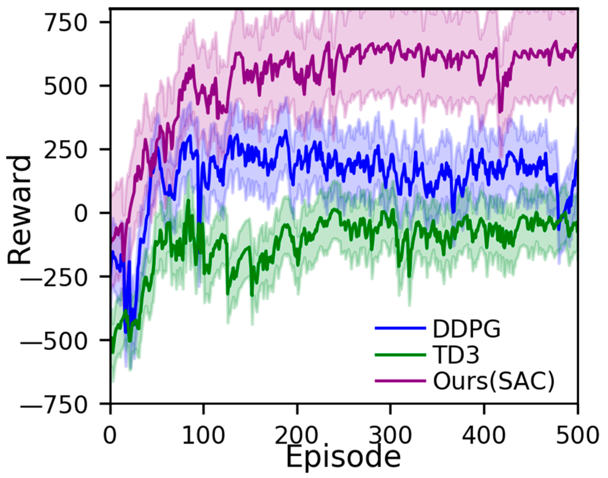
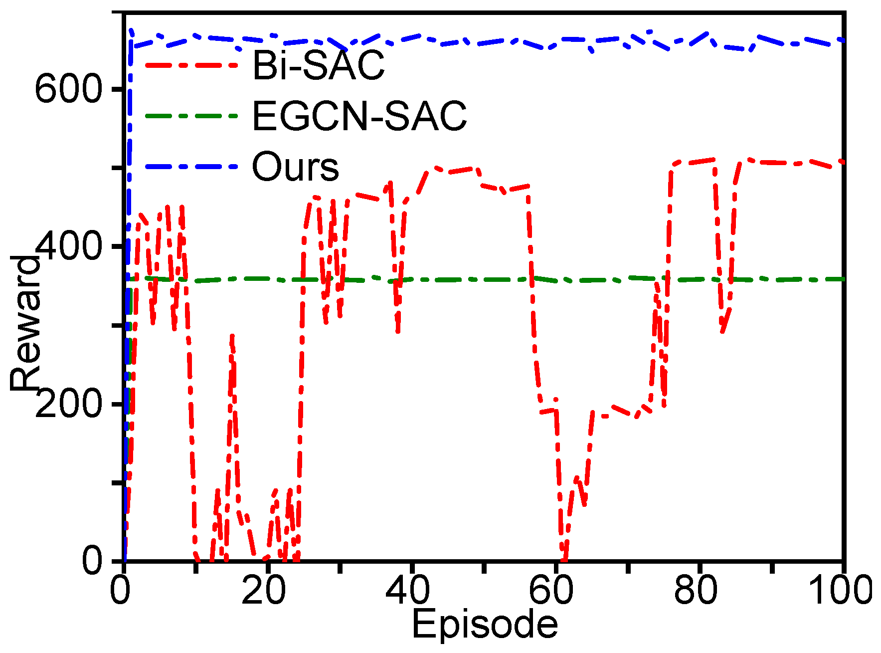
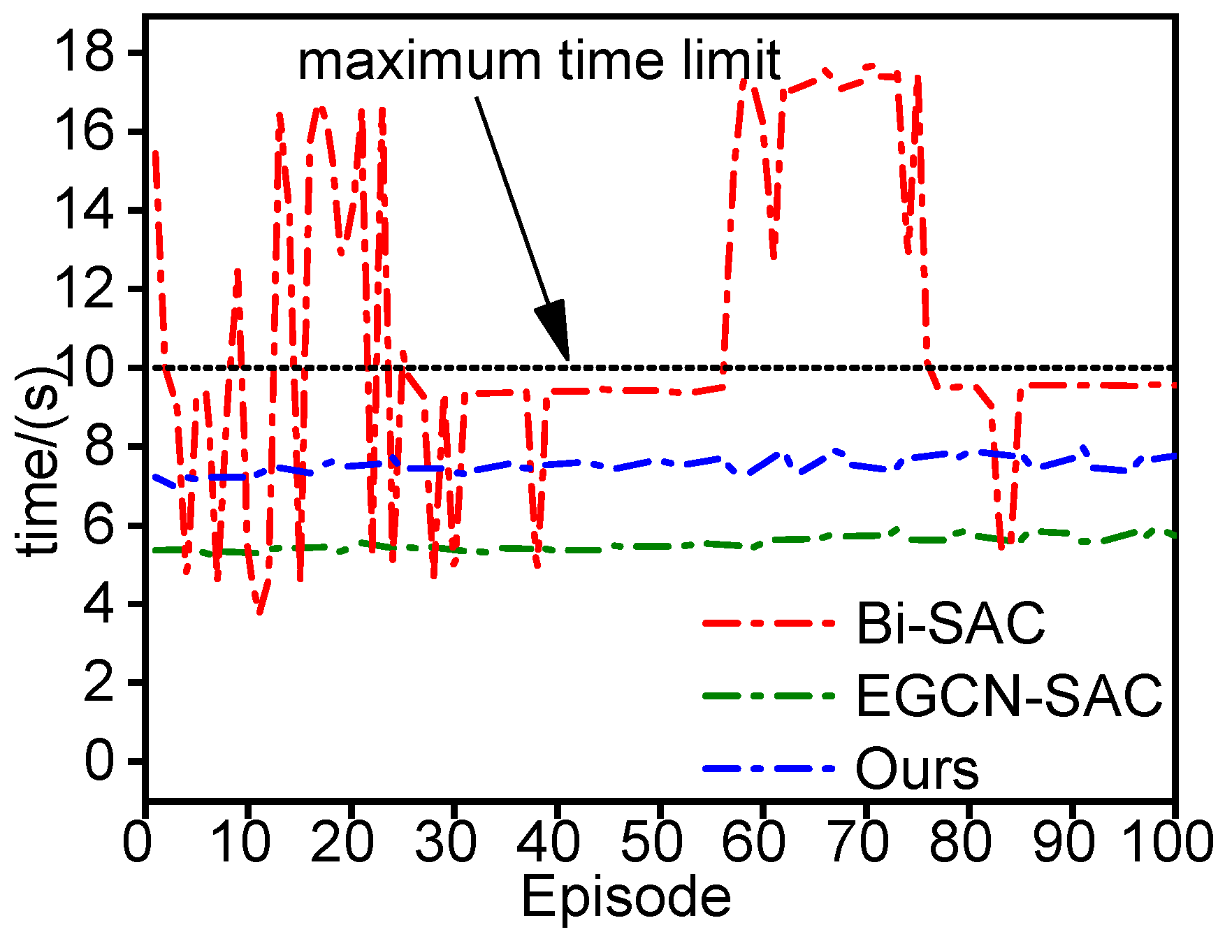
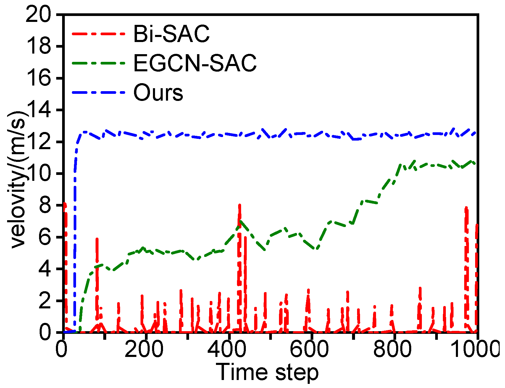
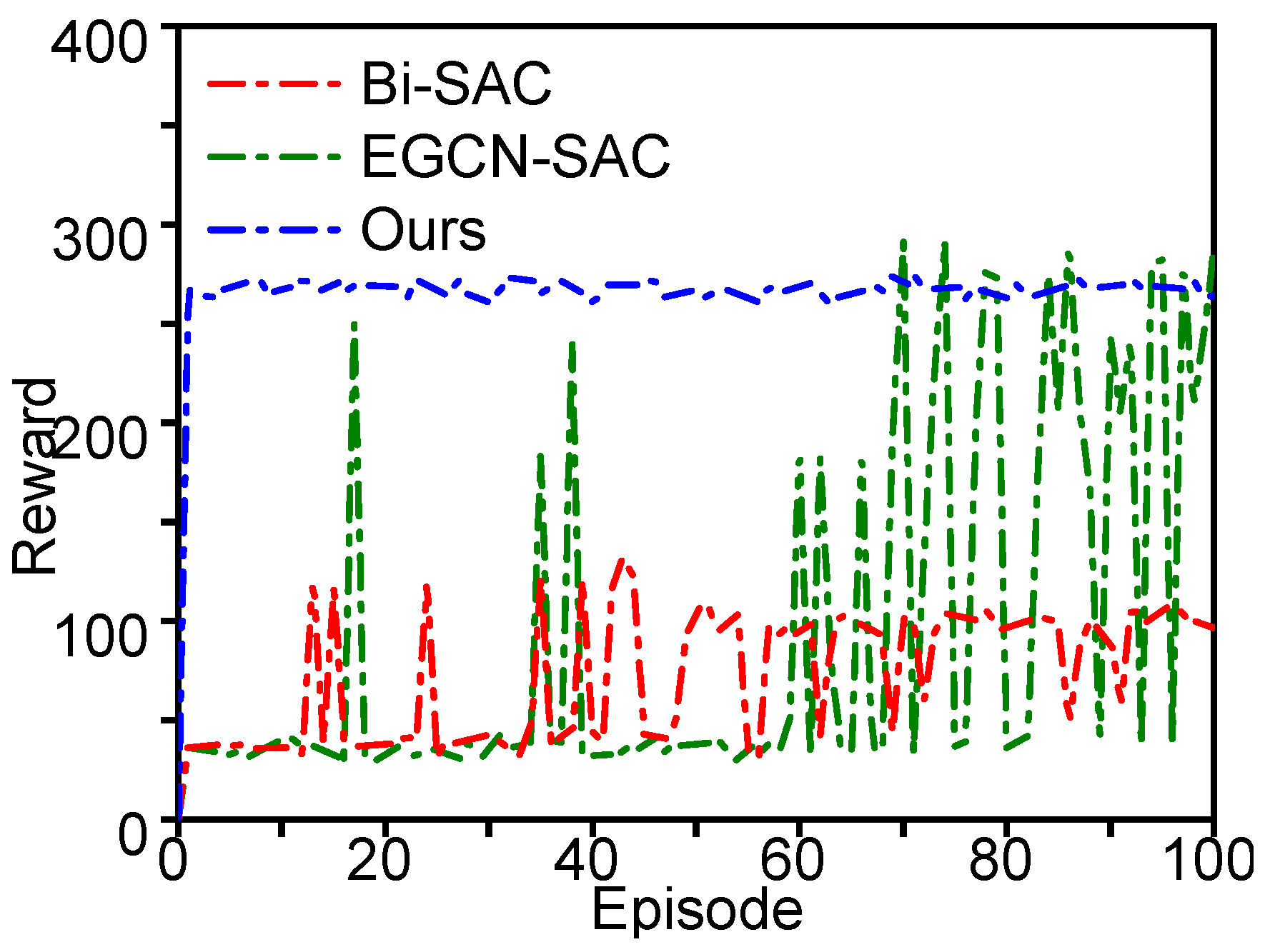
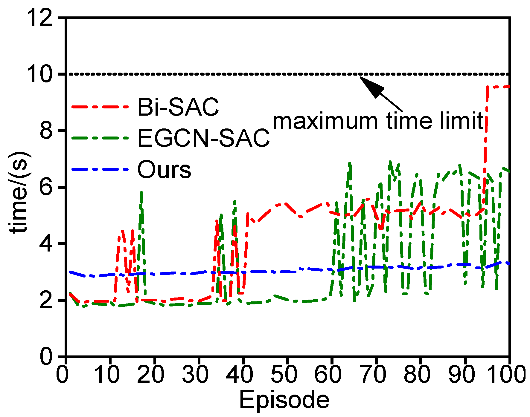
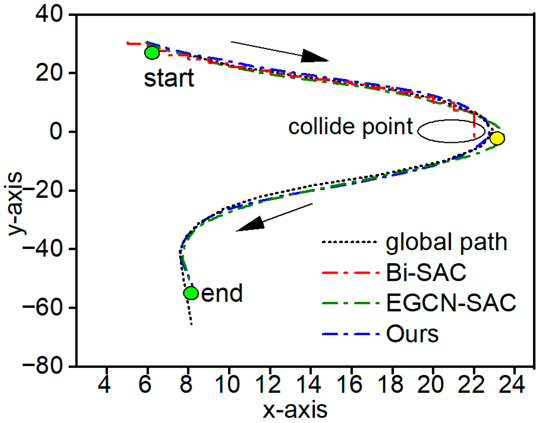
3.2.2. Experimental Results of Decision Model

Training results In order to verify the effectiveness of introducing vehicle trajectory prediction to the SAC decision model in this paper, controlled experiments were designed, which compared the reward curves of the following algorithms under 500 rounds of training: the algorithm in this paper (Ours), the SAC algorithm based on the prediction of the Bilstm model (Bi-SAC), the SAC algorithm based on the prediction of the EGCN model (EGCN-SAC), the and a SAC algorithm that does not incorporate any prediction trajectories (ONLY-SAC). (Since the poor prediction ability of the transformer encoder model itself was mentioned in Section 3.1.2, it will not be considered in this section.) The results of the reward curve comparison are shown in Figure 4.

Comparing the four curves, firstly, it can be judged that the inclusion of the predicted number of future trajectories of the vehicle in the SAC model can bring positive benefits to the decision-making ability of the autonomous vehicle. Secondly, compared with the other three trajectory prediction models, the algorithm in this paper obtains faster reward growth and significantly higher reward values. Although the reward value of the EGCN-SAC algorithm, which is in second place, is significantly higher than that of Bi-SAC and ONLY-SAC, the overall amplitude of the curves is too large, and the algorithm stability is not strong. From the above analysis, it shows that the present model is more helpful for the ego-vehicle to learn better driving performance in a shorter period of time.

In order to verify the effectiveness of the SAC decision-making algorithm designed in this paper, the present prediction model is applied to DDPG and TD3, two algorithms also based on the Actor-Critic framework, respectively, and the experimental results are shown in Figure 5 after 500 rounds of training:

Based on the reward curves, it can be seen that the SAC algorithm incorporating the trajectory prediction model significantly outperforms the other two algorithms both in terms of convergence speed and overall reward value. The possible reason for this is that both the DDPG and TD3 algorithms are based on deterministic strategies, whereas in this paper, 100 NPC vehicles are added to the training map, and the resulting environment is highly dynamic, leading to poorer robustness of their decisions. In contrast, the algorithm in this paper benefits from the entropy regularization mechanism of the SAC algorithm, which can effectively encourage the exploratory behavior of the ego-vehicles, and improve the overall decision-making effect and the stability of decision-making.

Test results In order to verify the performance of the algorithm in a dynamic environment, this paper constructs three dynamic simulation scenarios with interactivity in CARLA for testing (as shown in Figure 6) for straight line obstacle avoidance, traffic roundabout, and unprotected five-way intersection, and designs the obstacle vehicles in the environment to have an impact on the behavioral decisions of the ego-vehicles, where the red vehicle is the ego-vehicle, which is represented by ‘ego’, and the black vehicle is the obstacle vehicle, identified in the figure by the letters ‘A’, ‘B’, ‘C’, ‘D’ identification. In this case, the red vehicle is the ego-vehicle and the black vehicle is the obstacle vehicle around it, the blue solid arrow is the traveling direction of the ego-vehicle and the black dashed arrow is the traveling direction of the obstacle vehicle.

The test procedure was to increase the complexity of the dynamic scene by sequentially adding obstacle vehicles to the scene and to evaluate the decision-making performance of the self-vehicles during the interaction after the introduction of the predictive model. Each scene was tested 100 times and the performance of the algorithm in different complex dynamic scenes was evaluated using the following three metrics as shown in

Table 6. Test performance metrics.

Metrics	Explanation
Success rate	the percentage of autos successfully completing a prescribed route over multiple tests.
Crash rate	the percentage of crashes that occurred in multiple tests of the autocar.
Overtime rate	the percentage of autos exceeding the maximum time limit over multiple tests.

.

A. Linear Obstacle Avoidance

As shown in Figure 6a, in which A, B, C three obstacle vehicles are to be entered into the range of interest of the ego-vehicle to start the movement, in the ego-vehicle driving process, C obstacle car suddenly changed to the left to the ego-vehicle lane, placing it directly on the ego-vehicle’s originally traveled route of impact, and if the vehicle chooses to change lanes to overtake the vehicle in front of it, it will be possible to produce a potential collision with the A, B cars.

The test results are shown in

Table 7. Test result statistics in linear obstacle avoidance.

Model	Success Rate (%)	Crash Rate (%)	Overtime Rate (%)	Average Test Rewards	Average Test Time (s)
Ours	100	0	0	654.29	5.54
EGCN-SAC	100	0	0	354.96	7.52
Bi-SAC	69	1	30	336.78	10.84

, where both this paper’s algorithm and the EGCN-SAC algorithm obtained a 100% success rate and high average test rewards, while the Bi-SAC algorithm experienced multiple timeouts. From Figure 7 and Figure 8, it can be seen that the reward value and the time required during the testing of this paper’s algorithm and the EGCN-SAC algorithm are smoother, while the Bi-SAC algorithm has a significant decrease in the reward value due to the occurrence of multiple timeouts and collisions. Additionally compared to the EGCN-SAC algorithm, the algorithm in this paper has a higher reward value and requires less test time under the same driving conditions, giving it higher passing efficiency.

Further analyzing the test situation of a single round, when the obstacle vehicle C urgently inserts into the lane of the ego-vehicle, it can be seen from Figure 9 and Figure 10 that the three algorithms adopt different obstacle avoidance strategies: the vehicle of in the EGCN-SAC algorithm fails to return to the original lane after switching to the neighboring lanes, and instead, it travels in the direction of the obstacle vehicle A, failing to reach its own target speed. In this paper, after adding the predicted number of each obstacle vehicle, we find that the future speed trend of obstacle vehicle A is always smaller than that of its own vehicle, so it completes the lane change to overtake vehicle C with a more stable speed and returns to the original lane quickly, reflecting a higher passing efficiency. The Bi-SAC algorithm’s vehicle chooses a more conservative route, always follows vehicle C in this lane, and completes the whole journey through frequent acceleration and deceleration after unsuccessful attempts to overtake, and because of the moderate speed maintained at a low level, the vehicle is not able to reach its own target speed. The overall reward value is lower because the speed is moderately maintained at a lower level.

B. Roundabout

In the traffic circle scenario shown in Figure 6b, obstacle vehicles A and B are located in the range of interest of the ego-vehicle. When the ego-vehicle starts traveling around the traffic circle, obstacle vehicle B inserts into the ego-vehicle’s traveling path from one side, and obstacle vehicle A converges from the north entrance of the traffic circle. The difficulty of the traffic circle scenario lies in the large curvature and the large number of switchbacks, which makes it easy for the ego-vehicle to lose the ability to track the global path while avoiding the obstacle vehicle.

In the results shown in

Table 8. Test result statistics in a roundabout.

Model	Success Rate (%)	Crash Rate (%)	Overtime Rate (%)	Average Test Rewards	Average Test Time (s)
Ours	100	0	0	267.64	3.06
EGCN-SAC	60	40	0	92.83	3.26
Bi-SAC	30	70	0	73.01	4.29

, it can be seen that in the traffic circle scenario, the algorithm proposed in this paper is able to complete the route successfully, while the EGCN-SAC and Bi-SAC algorithms collide to varying degrees. Figure 11 shows that the reward changes of this paper’s algorithm are relatively smooth during the 100 rounds of testing, while the rewards of the other two algorithms fluctuate more. When the reward value is low, it corresponds to a shorter test time in Figure 12, indicating that at this point a collision with an obstacle vehicle occurs during the movement, resulting in early termination of the round.

As shown in Figure 13, the arrows indicate the direction of the global path, and the EGCN-SAC algorithm has difficulty in fully tracking the global path at the point of maximum curvature of the traffic circle (yellow point) in a single round of testing, while the Bi-SAC algorithm is unable to predict the speed and location of the obstacle vehicle A approaching from the side in the event of a collision at this point. As shown in Figure 14, the algorithm in this paper adopts an aggressive strategy after predicting the brief signs of acceleration of vehicle A, accelerating before traveling to the point to ensure passage, while the EGCN-SAC algorithm chooses to reduce the speed appropriately, and both algorithms are able to quickly restore a smooth speed after passing the point. It can be seen that the algorithm in this paper has a shorter test time and higher passing efficiency.

In order to better reflect the superiority of the prediction algorithm in the decision validation environment, we output the comparison results of the actual trajectories of obstacle vehicles A and B in this scenario with the predicted trajectories, as shown in Figure 15 and Figure 16. From the comparison results, it can be seen that even in complex scenarios with large changes in path curvature, the algorithm in this paper is still able to achieve a more accurate trajectory tracking, which provides more reliable prediction support for the subsequent decision-making algorithm.

C. Unprotected Five-way Intersection

In the five-turn intersection scenario shown in Figure 6c, this paper sets four points that may conflict with the traveling route of the ego-vehicle. Among them, vehicles A, B, and D are traveling straight, which may form a positive conflict with the traveling route of the ego-vehicle; while vehicle C executes a left turn and merges into the same target lane with the ego-vehicle after the turn, and once the ego-vehicle completes the turn, only vehicle C is still in the range of interest of the ego-vehicle.

Considering the multiple interacting intelligences involved in the scenario; in order to more comprehensively verify the robustness of the algorithms to complex scenarios, this paper gradually increases the number of obstacle vehicles and observes the performance changes of the three algorithms in the test. As the number of obstacle vehicles increases, the target points also increase, which makes the probability of collision of ego-vehicles in avoidance rise. In addition, in complex scenarios, the autonomous vehicle may also experience the “robot freeze” phenomenon, i.e., it slackens off at a very low speed in order to avoid a collision, which leads to an increase in the timeout rate.

As can be seen from the test results in

Table 9. Test result statistics in an unprotected five-way intersection.

Obstacle Vehicle Setup	Model	Success Rate (%)	Crash Rate (%)	Overtime Rate (%)	Average Test Rewards	Average Test Time (s)
A, C	Ours	99	1	0	419.71	6.37
	EGCN-SAC	100	0	0	409.75	7.00
	Bi-SAC	97	3	0	228.68	8.56
A, C, D	Ours	95	5	0	382.67	5.28
	EGCN-SAC	90	10	0	251.11	2.93
	Bi-SAC	75	25	0	205.11	4.94
A, B, C, D	Ours	76	24	0	286.36	7.00
	EGCN-SAC	65	35	0	175.31	2.99
	Bi-SAC	54	30	16	122.62	3.27

, with the gradual increase of obstacle cars in the scene, the performance of the three algorithms decreases, and the analysis found that the additional vehicles B and D entered the target vehicle’s range of interest in turn, during which the state space of the decision-making algorithm changed, and consequently the algorithm underwent adaptive adjustments in generating the decision values, and therefore the algorithm may have some limitations in responding to dynamic scenarios, and may not be able to make an effective response in a timely manner. Specifically, the success rate of this paper’s algorithm decreases by 4% and 19% in turn, and the average test reward decreases by 8% and 25.2% in turn, the success rate of the EGCN-SAC algorithm decreases by 10% and 25% in turn and the average test reward decreases by 38.7%, 25.2% in turn, the success rate of the Bi-SAC algorithm decreases by 22% and 21%, and the average test reward decreases by 10.3% and 40.2% in turn, It can be seen that adding obstacle vehicle B is more likely to have an impact on the autoroute than adding obstacle vehicle D. The algorithm in this paper is clearly more robust to the complexity of the scenario.

4. Conclusions

In order to overcome the influence of dynamic traffic participants on the decision-making of the ego-vehicle in the traffic environment, this paper proposes an autopilot learning strategy based on spatial-temporal feature prediction. The strategy establishes spatial relationships between the vehicle and the surrounding traffic participants, and establishes temporal relationships with the input of historical trajectory points, so as to predict the trajectories of the vehicle and the surrounding participants, and uses reinforcement learning as the automatic driving strategy, and the predicted trajectory points will expand the state space of the reinforcement learning, so as to enable the vehicle to have the ability to “foresee” the behavior of future traffic participants, and then realize effective obstacle avoidance in dynamic environments. The predicted trajectory points will expand the state space of reinforcement learning, so that the vehicle has the ability to “anticipate” the behavior of future traffic participants, and then realize effective obstacle avoidance in dynamic environments.

Simulation results show that the spatial-temporal feature-based prediction model proposed in this paper has a high prediction accuracy. Compared to the two temporal feature predictions, Bilstm and transformer encoder, in the high-speed scenario, the prediction model ADE of this paper decreased by 55% and 80%, and the FDE decreased by 34% and 75%, respectively, and in the dry-road scenario, the prediction model ADE of this paper decreased by 54% and 84%, and the FDE decreased by 54% and 80%, respectively. Compared with the traditional spatial-temporal fusion-based prediction algorithm EGCN, the ADE of this paper’s prediction model decreased by 45% and FDE decreased by 43% in the high-speed scenario, and the ADE of this paper’s prediction model decreased by 33% and FDE decreased by 28% in the arterial road scenario. In the prediction-based decision-making task, this paper’s algorithm shows the highest success rate, the lowest timeout and collision rates, and the highest average test rewards compared to the Bi-SAC and EGCN-SAC algorithms in the three dynamic scenarios. This shows that the decision-making algorithm based on the prediction algorithm in this paper is able to use safer and more efficient strategies to complete the driving task.

Future research will be extended to model other dynamic participants with specific behavioral patterns such as pedestrians and non-motorized vehicles to further improve trajectory prediction for other traffic participants with dynamic, uncertain behavior. In addition, future work will also aim to apply these algorithms to real-vehicle validation in practical road scenarios to further evaluate the performance and feasibility of the models in different driving conditions.

References

1. Xie, G.T. Research on Dynamic Environment Cognition Method for Intelligent Vehicles Under Uncertainty Conditions. Ph.D. Thesis, Hefei University of Technology, Hefei, China, 2018. [Google Scholar]
2. Xu, J.; Pei, X.; Fei, X.; Yang, B.; Fang, Z. Incorporating vehicle trajectory prediction for learning autonomous driving decision. J. Automot. Saf. Energy Conserv. 2022, 13, 317–324. [Google Scholar]
3. Lipton, Z.C.; Berkowitz, J.; Elkan, C. A critical review of recurrent neural networks for sequence learning. arXiv 2015, arXiv:1506.00019. [Google Scholar]
4. Gao, J.; Sun, C.; Zhao, H.; Shen, Y.; Anguelov, D.; Li, C.; Schmid, C. VectorNet: Encoding HD maps and agent dynamics from vectorized representation. In Proceedings of the IEEE/CVF Conference on Computer Vision and Pattern Recognition, Seattle, WA, USA, 14–19 June 2020. [Google Scholar]
5. Wu, Z.; Pan, S.; Chen, F.; Long, G.; Zhang, C.; Philip, S.Y. A comprehensive survey on graph neural networks. IEEE Trans. Neural Netw. Learn. Syst. 2021, 32, 4–24. [Google Scholar] [CrossRef] [PubMed]
6. Ji, X.; Fei, C.; He, X.; Liu, Y.; Liu, Y. Driving intention recognition and vehicle trajectory prediction based on LSTM network. Chin. J. Highway 2019, 32, 34–42. [Google Scholar] [CrossRef]
7. Zhou, Y.; Xia, M.; Zhu, B. Research on multimodal vehicle trajectory prediction method considering multiple types of traffic participants in urban road scenarios. Automot. Eng. 2024, 46, 396–406. [Google Scholar] [CrossRef]
8. Sheng, Z.; Xu, Y.; Xue, S.; Li, D. Graph-based spatial-temporal convolutional network for vehicle trajectory prediction in autonomous driving. IEEE Trans. Intell. Transp. Syst. 2022, 23, 17654–17665. [Google Scholar] [CrossRef]
9. Xiong, L.; Kang, Y.; Zhang, P.; Zhu, C.; Yu, Z. Research on behavioral decision-making system for driverless vehicles. Automot. Technol. 2018, 1–9. [Google Scholar] [CrossRef]
10. Bansal, M.; Krizhevsky, A.; Ogale, A. Chauffeurnet: Learning to drive by imitating the best and synthesizing the worst. arXiv 2018, arXiv:1812.03079. [Google Scholar]
11. Jin, L.; Han, G.; Xie, X.; Guo, B.; Liu, G.; Zhu, W. A review of research on automatic driving decision-making based on reinforcement learning. Automot. Eng. 2023, 45, 527–540. [Google Scholar] [CrossRef]
12. Huang, C.; Zhang, R.; Ouyang, M.; Wei, P.; Lin, J.; Su, J.; Lin, L. Deductive reinforcement learning for visual autonomous urban driving navigation. IEEE Trans. Neural Netw. Learn. Syst. 2021, 32, 5379–5391. [Google Scholar] [CrossRef] [PubMed]
13. Gao, Z.; Sun, T.; Xiao, H. Decision-making method for vehicle longitudinal automatic driving based on reinforcement Q-learning. Int. J. Adv. Robot. Syst. 2019, 16, 1729881419853185. [Google Scholar] [CrossRef]
14. Zhang, Z.; Huang, D.; Huang, C.; Wang, L.; Liu, J.; Chen, F.; Xu, H.; Gao, X.; Li, Q.; Zhou, Y.; et al. TD3 algorithm improvement and merging strategy learning for self-driving cars. J. Mech. Eng. 2023, 59, 224–234. [Google Scholar]
15. Tinghan, W.; Yugong, L.; Jinxin, L.; Li, K. End-to-end autonomous driving strategy based on deep deterministic policy gradient algorithm considering state distribution. J. Tsinghua Univ. (Nat. Sci. Ed.) 2021, 61, 881–888. [Google Scholar] [CrossRef]
16. Zhang, Z.; Liniger, A.; Dai, D.; Yu, F.; Van Gool, L. End-to-end urban driving by imitating a reinforcement learning coach. In Proceedings of the IEEE/CVF International Conference on Computer Vision, Montreal, BC, Canada, 11–17 October 2021. [Google Scholar]
17. Ghadi, N.; Deo, T.Y. Safe Navigation: Training Autonomous Vehicles using Deep Reinforcement Learning in CARLA. arXiv 2023, arXiv:2311.10735. [Google Scholar]
18. Wang, M.; Tang, X.; Yang, K.; Li, G.; Hu, X. A motion planning method for self-driving vehicles considering predictive risk. Automot. Eng. 2023, 45, 1362–1372+1407. [Google Scholar] [CrossRef]
19. Haarnoja, T.; Zhou, A.; Hartikainen, K.; Tucker, G.; Ha, S.; Tan, J.; Kumar, V.; Zhu, H.; Gupta, A.; Abbeel, P.; et al. Soft actor-critic algorithms and applications. arXiv 2018, arXiv:1812.05905. [Google Scholar]
20. Alexiadis, V.; Colyar, J.; Halkias, J.; Hranac, R.; McHale, G. The next generation simulation program. ITE J. 2004, 74, 22. [Google Scholar]
21. Pareja, A.; Domeniconi, G.; Chen, J.; Ma, T.; Suzumura, T.; Kanezashi, H.; Kaler, T.; Schardl, T.B.; Leiserson, C.E. Evolvegcn: Evolving graph convolutional networks for dynamic graphs. Proc. AAAI Conf. Artif. Intell. 2020, 34, 2276–2283. [Google Scholar] [CrossRef]
22. Dosovitskiy, A.; Ros, G.; Codevilla, F.; Lopez, A.; Koltun, V. CARLA: An open urban driving simulator. In Conference on Robot Learning; PMLR: Birmingham, UK, 2017. [Google Scholar]
Figure 1. Overall structure.
Applsci 14 11913 g001
Figure 2. Encoder-decoder network.
Applsci 14 11913 g002
Figure 3. Flowchart of the SAC algorithm.
Applsci 14 11913 g003
Figure 4. Comparison curve of SAC algorithm training rewards under different prediction models.
Applsci 14 11913 g004
Figure 5. Comparison curve of this paper’s algorithm with other reinforcement learning training rewards.
Applsci 14 11913 g005
Figure 6. Three simulation test scenarios built in CARLA.
Applsci 14 11913 g006
Figure 7. Test reward change curves.
Applsci 14 11913 g007
Figure 8. Test time change curves.
Applsci 14 11913 g008
Figure 9. Comparison of the path offsets.
Applsci 14 11913 g009
Figure 10. Comparison of the ego-vehicle speeds.
Applsci 14 11913 g010
Figure 11. Test reward change curve.
Applsci 14 11913 g011
Figure 12. Test time change curve.
Applsci 14 11913 g012
Figure 13. Comparison of traveling tracks.
Applsci 14 11913 g013
Figure 14. Comparison of the ego-vehicle speeds.
Applsci 14 11913 g014
Figure 15. Comparison of actual and predicted trajectories of obstacle vehicle A.
Applsci 14 11913 g015
Figure 16. Comparison of actual and predicted trajectories of obstacle vehicle B.
Applsci 14 11913 g016