A Lightweight Kernel Density Estimation and Adaptive Synthetic Sampling Method for Fault Diagnosis of Rotating Machinery with Imbalanced Data

Abstract

Rotating machinery is widely used across various industries, making its reliable operation crucial for industrial production. However, in real-world settings, intelligent fault diagnosis faces challenges due to imbalanced fault data and the complexity of neural network models. These challenges are particularly pronounced when defining decision boundaries accurately and managing limited computational resources in real-time machine monitoring. To address these issues, this study presents KDE-ADASYN-based MobileNet with SENet (KAMS), a lightweight convolutional neural network designed for fault diagnosis in rotating machinery. KAMS effectively handles data imbalances commonly found in industrial applications and is optimized for real-time monitoring. The model employs the Kernel Density Estimation Adaptive Synthetic Sampling (KDE-ADASYN) algorithm for oversampling to balance the data, applies fast Fourier transform (FFT) to convert time-domain signals into frequency-domain signals, and utilizes a 1D-MobileNet network enhanced with a Squeeze-and-Excitation (SE) block for feature extraction and fault diagnosis. Experimental results across datasets with varying imbalance ratios demonstrate that KAMS achieves excellent performance, maintaining nearly 90% accuracy even on highly imbalanced datasets. Comparative experiments further demonstrate that KAMS not only delivers exceptional diagnostic performance but also significantly reduces network parameters and computational resource requirements.

1. Introduction

The rapid advancement of modern industry has led to the extensive use of machinery and equipment across sectors such as manufacturing, transportation, and aerospace [1]. Rotating mechanical components are vital to the operation of most machinery, and their condition directly affects both performance and lifespan [2]. Failures in these components can cause significant equipment damage and may even result in safety hazards [3]. Rolling bearings are essential components in rotating machinery, and their damage severity can be comprehensively evaluated based on the location, type, and vibration characteristics of the damage. Consequently, accurate and timely intelligent diagnosis of rotating machinery is crucial for preventing failures, reducing maintenance costs, and enhancing production efficiency [4,5].

Fault diagnosis of rotating machinery is generally categorized into model-based and data-driven methods [6]. Model-based approaches use physical or mathematical models to describe the normal operating state of bearings by analyzing discrepancies between the model’s predictions and the actual operational data [7]. However, feature extraction and analysis in these methods heavily rely on the prior knowledge of signal processing experts [8]. With the rise of sensing technology and artificial intelligence (AI), real-time monitoring has produced vast quantities of data, and data-driven methods, particularly deep learning, have become dominant in machine fault diagnosis due to their ability to mine information and extract features from large datasets [9,10]. Deep learning methods hold great promise for fault detection, thanks to their powerful pattern recognition and feature extraction capabilities, as well as their ability to handle high-dimensional nonlinear data. These strengths have attracted significant attention from researchers, as deep learning-based methods offer potential for improving production efficiency and reducing operational and maintenance costs across multiple industries.

Deep learning fault diagnosis methods utilize deep neural networks to automatically extract features from large-scale data, enabling high-precision fault classification [11]. Typical deep learning models include convolutional neural networks (CNNs), recurrent neural networks (RNNs), graph neural networks (GNNs), and their optimized variants. For instance, Gong et al. [12] employed a CNN to extract effective features from raw data, which were then fed into a support vector machine (SVM) for fault classification. Liu [13] proposed a bearing fault diagnosis model based on an ensemble of CNNs, which improved fault information collection and reduced information loss. In intelligent engine diagnostics, a progressive adaptive sparse attention mechanism has been applied in high-power diesel engine fault detection, demonstrating the effectiveness of attention-guided feature extraction [14]. It is important to note, however, that the outstanding performance of deep learning models depends on the availability of rich data. Effective training requires access to diverse fault data and a relatively balanced distribution of samples. Unfortunately, rotating machinery typically operates under normal conditions most of the time, with fault states occurring only briefly due to cost and safety considerations. This results in a larger volume of normal data compared to fault data, creating an imbalance that makes it difficult for deep learning models to accurately define decision boundaries [15].

Recently, data imbalance has significantly affected deep learning-based fault diagnosis, leading researchers to explore methods for diagnosing faults in imbalanced datasets. Liu et al. [16] proposed a kernel valve fault critical point prediction method, integrating multiple sensitive parameters to address the scarcity of fault samples. Wang et al. [17] applied deep generative adversarial networks (GANs) to generate additional samples and balance the data before classifying bearing faults. However, GANs face challenges like low training accuracy and high computational demands. Data augmentation techniques are still widely used for balancing datasets, with the synthetic minority oversampling technique (SMOTE) and its variants being particularly common [18]. Swana et al. [19] applied SMOTE to synthesize motor fault samples, enhancing classifier performance. Compared to a GAN, SMOTE requires fewer computational resources and can generate a large number of fault samples, meeting the needs of intelligent diagnostic models [20]. SMOTE has been improved in subsequent algorithms, which have reduced the generation of ineffective samples, as shown in methods like LR-SMOTE and Borderline-SMOTE [21,22]. However, in areas where minority and majority class samples overlap, SMOTE may unintentionally generate new samples within the majority class, reducing classification performance. To address this issue, He et al. introduced the adaptive synthetic (ADASYN) algorithm in 2008. The core concept of ADASYN is to assign different weights to minority class samples and generate new samples based on these weights, effectively mitigating class imbalance [23]. Despite its advantages, ADASYN may still cause ambiguous decision boundaries, especially when handling multiple minority classes with varying sample sizes, increasing the risk of misclassification [24,25]. In 2015, Tang et al. proposed the Kernel ADASYN method, enhancing the ADASYN approach by incorporating kernel density estimation. This method calculates the probability density of minority class samples and assigns weights according to sample importance [26]. By improving the quality of minority class samples near decision boundaries, Kernel ADASYN enhances the accuracy of downstream classifiers [27]. However, current research on fault diagnosis of rotating machinery mainly focuses on the imbalance between normal and faulty samples, often neglecting the uneven distribution of samples across different fault types. For example, Li et al. found that Dataset C contains 1500 normal samples, but each of the three distinct fault types is represented by only 300 samples [28].

A further challenge of using deep learning for intelligent fault diagnosis is the high computational resource consumption of the models, which poses significant disadvantages for real-time monitoring applications. To improve real-time monitoring and applications in movable machinery, deep learning-based fault diagnosis models must simplify complexity, reduce parameters, and progress towards lightweight development [29]. Since 2016, several lightweight network architectures have been proposed. SqueezeNet, for example, aims to drastically reduce the number of model parameters while maintaining accuracy comparable to larger, more complex models [30]. ShuffleNet, designed for mobile and embedded devices, increases network efficiency through channel shuffling and grouped convolutions [31]. MobileNet, introduced by Howard, is another representative lightweight convolutional neural network that significantly reduces model size while preserving accuracy, comparable to traditional networks like CNN and visual geometry group (VGG) networks [32]. In the field of fault diagnosis, MobileNet has produced notable research results. Yu et al. developed a fault diagnosis model based on MobileNet, implementing an end-to-end intelligent fault classification and diagnosis application [33]. Similarly, Landi et al. [34] proposed a low-complexity MobileNet neural network for classifying different bearing fault vibration signals, achieving over 99% classification accuracy even under various interference conditions. However, lightweight convolutional networks, such as MobileNet, are mainly used for image processing, and studies on their application in fault diagnosis of one-dimensional signals in rotating machinery remain relatively scarce.

Existing deep learning models designed to address data imbalance in rotating machinery fault diagnosis face three main challenges.

(1)

Failure to account for the varying quantities of different fault types during model training limits the ability to handle the randomness of fault types and quantities in real-world scenarios.

(2)

The lack of high-precision lightweight models for fault diagnosis of one-dimensional signals in rotating machinery limits their application in real-time monitoring within prognostics and health management (PHM) systems.

(3)

Traditional oversampling methods struggle to generate enough high-quality samples near class boundaries, increasing the risk of misclassification around decision boundaries.

To address these challenges, this paper introduces the KDE-ADASYN algorithm, which utilizes a Gaussian kernel function to balance the data. Additionally, a lightweight 1D convolutional neural network with an attention mechanism is proposed, designed to enhance diagnostic performance while minimizing computational resource usage. The main contributions of this research are as follows:

(1)

The Gaussian kernel-based KDE-ADASYN algorithm calculates the probability density distribution and weight of each minority class sample, adjusts the number of new samples generated near various minority class boundaries, and improves the classifier’s decision boundary accuracy in complex imbalanced data scenarios.

(2)

A lightweight 1D CNN for fault diagnosis is developed, incorporating MobileNet with an embedded SE block. The attention mechanism enhances feature extraction, and the lightweight network drastically reduces model parameters and conserves computational resources, making it ideal for mobile machinery and real-time monitoring applications.

(3)

Training sets with varying sample sizes for different fault types are constructed using the PU and HUST datasets, addressing the challenge of model applicability in real-world conditions.

The remainder of this paper is organized as follows: Section 2 provides a detailed explanation of the proposed KDE-ADASYN-based MobileNet with SENet (KAMS) model. Section 3 focuses on the experimental validation and the analysis of the results. Finally, Section 4 summarizes the conclusions of this paper.

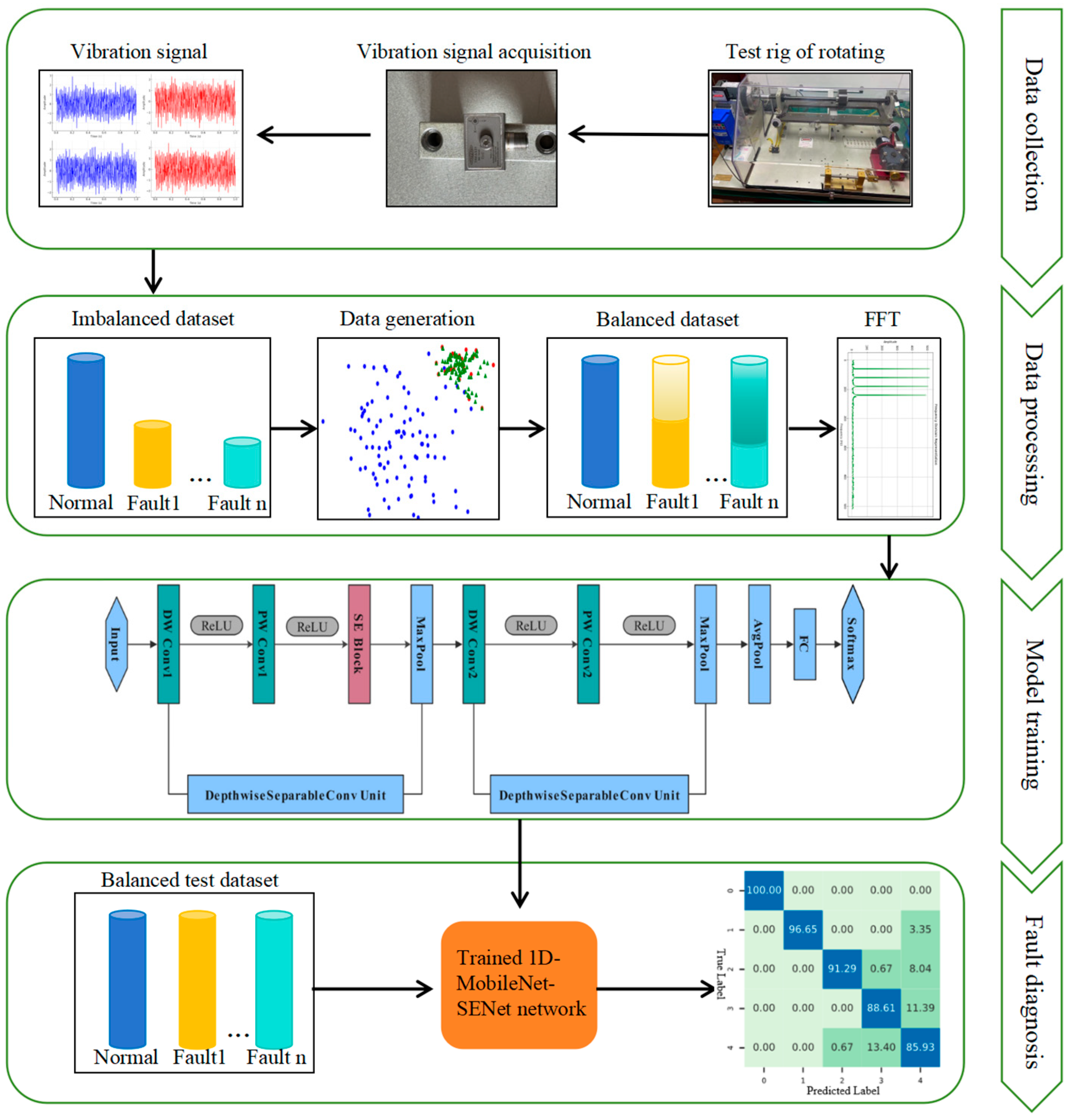
2. The Proposed Methods

To enhance the performance of fault diagnosis models for rotating machinery under complex imbalanced data conditions and to enable real-time monitoring in mobile mechanical equipment, the KAMS lightweight fault diagnosis model is proposed, as illustrated in Figure 1. First, sensors collect vibration signals in real time, converting mechanical vibrations into electrical signals for data acquisition and analysis. The KDE-ADASYN algorithm, based on a Gaussian kernel function, is then applied to augment the minority class samples. Next, fast Fourier transform (FFT) technology is used to convert the vibration signals from the time domain to the frequency domain. Finally, the balanced samples are used to train a lightweight 1D-MobileNet model embedded with an attention mechanism. This approach combines advanced data augmentation techniques with efficient deep learning models, creating a robust and practical fault diagnosis system for rotating machinery, particularly in scenarios with imbalanced data.

2.1. KDE-ADASYN

The KDE-ADASYN algorithm is utilized to address more complex data imbalance issues. This algorithm generates new samples that maintain the original probability distribution of the minority class while simultaneously increasing the quantity and improving the quality of samples near decision boundaries. The specific steps are as follows:

Step 1: Define the number of minority class samples as $N_{\min }$, the number of majority class samples as $N_{\max }$, and the total number of samples as $N$. For each minority class vibration signal sample, use the Euclidean distance to find its $K$ nearest neighbors. Then, calculate the ratio of majority class samples within these $K$ neighbors to obtain the weight $r_i$, which reflects the degree of class imbalance around each sample.

$$r_i={\displaystyle \frac{Number of majority class samples}{Total number of K-nearest neighbors}}$$

(1)

Next, normalize $r_i$ as follows:

$${\widehat{r}}_i={\displaystyle \frac{r_i}{{\displaystyle {\sum }_{i=1}^{N_{\min }}{r}_i}}}$$

(2)

Step 2: For each minority class vibration signal sample, use kernel density estimation to obtain the probability density function of the minority class samples.

$$p\left(x\right)={\displaystyle \frac{1}{N_{\min }+h}}{\displaystyle {\sum }_{i=1}^{N_{\min }}K}\left({\displaystyle \frac{x-x_i}{h}}\right)$$

(3)

where $h$ is the bandwidth parameter and $K$ is the kernel function. In this paper, the Gaussian kernel is used in the following equation:

$$G\left(x\right)={\displaystyle \frac{1}{{\left(\sqrt{2\pi }h\right)}^d}}\exp \left(-{\displaystyle \frac{1}{2}}{\displaystyle \frac{{\left(x-x_i\right)}^T\left(x-x_i\right)}{h}}\right)$$

(4)

Therefore, Equation (3) can be rewritten as

$$p\left(x\right)={\displaystyle \frac{1}{N_{\min }+h}}{\displaystyle {\sum }_{i=1}^{N_{\min }}G\left(x\right)}$$

(5)

By introducing the normalized weight coefficient ${\widehat{r}}_i$, the weighted probability density distribution of the minority class samples is obtained:

$$\widehat{p}\left(x\right)={\displaystyle \frac{1}{N_{\min }+h}}{\displaystyle {\sum }_{i=1}^{N_{\min }}{\widehat{r}}_{i}G\left(x\right)}$$

(6)

Step 3: Calculate the total number of new samples that need to be generated:

$$G=\left(N_{\max }-N_{\min }\right)\times \beta$$

(7)

where $\beta$ is a custom parameter within the range $\left[0,1\right]$.

Step 4: Based on the probability density distribution obtained from Equation (6), new samples are generated through sampling until the number of newly generated minority class samples reaches $G$. These new samples conform to the weighted probability distribution of the original minority class samples.

2.2. 1D-SENet Network

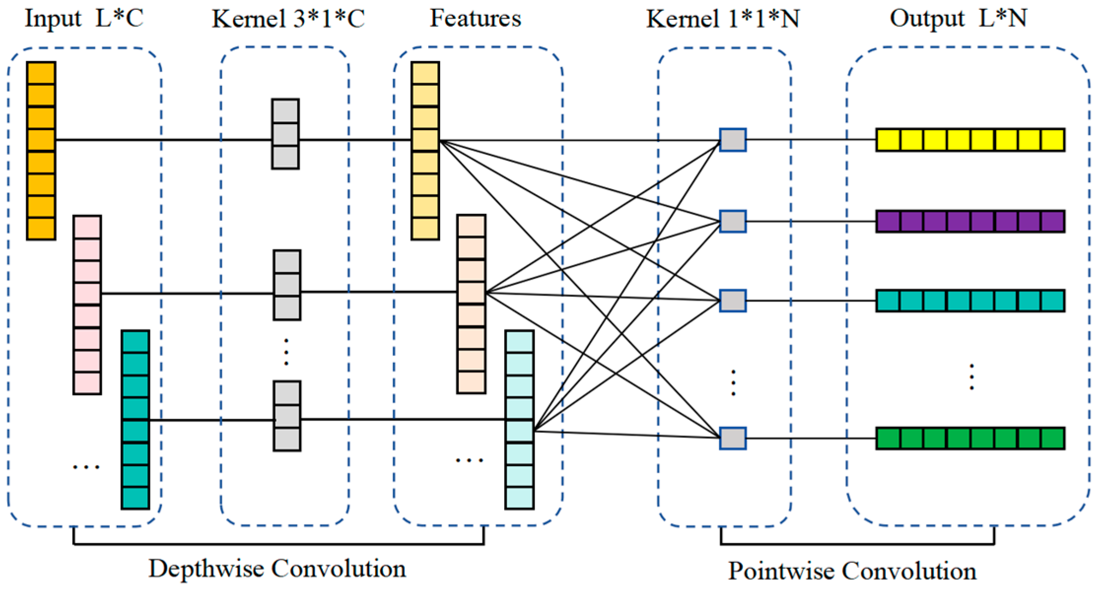
SENet is a channel attention mechanism designed to enhance the feature extraction capabilities of convolutional neural networks. By analyzing and processing the relationships between feature channels, SENet selectively learns the most important feature information and determines the significance of each channel. This allows for the diagnostic model to adaptively adjust the weight of each channel, suppressing irrelevant features and amplifying those most relevant to the task at hand. Consequently, the model’s diagnostic classification accuracy is significantly improved [35].

The basic structure of SENet is shown in Figure 2. The SE block is the core component of SENet and can be embedded into various convolutional neural networks as a module. The SE block consists of two main stages: Squeeze and Excitation. The one-dimensional fault sample signal $X\in R^{C^{\prime }\times L^{\prime }}$ undergoes a convolution operation to obtain $U\in R^{C\times L}$, where $C$ represents the number of channels and $L$ represents the length of the sample signal. The specific calculation method is as follows:

$$u_i=v_i\times X={\displaystyle {\sum }_{j=1}^{C^{\prime }}{v}_i^k\cdot x^j}$$

(8)

where $u_i$ represents the $i$-th channel of the fault sample signal, $v_i^k$ represents the $i$-th input of the $k$-th convolutional kernel, and $x^j$ represents the $j$-th channel of $X$.

For one-dimensional signals, the Squeeze operation performs global average pooling on the features of each channel to obtain a $1\times C$ vector, thereby capturing the overall characteristics and global information of each channel. This process is represented as follows:

$$z_c={\displaystyle \frac{1}{L}}{\displaystyle {\sum }_{i=1}^L{u}_c}\left(i\right)$$

(9)

where $z_c$ is the global average pooling result of the $c$-th channel, and $u_c\left(i\right)$ is the value at position $i$ of the $c$-th channel.

The Excitation operation captures the dependencies between channels through two fully connected layers and a nonlinear activation function, adaptively adjusting the weights of the channels. This enhances important feature channels and suppresses unimportant ones, as detailed below:

$$s=\sigma \left(W_2\delta \left(W_{1}z\right)\right)$$

(10)

where $s$ is the output channel weight vector with a length of $C$, $W_1\in R^{{\displaystyle \frac{C}{r}}\times C}$ and $W_2\in R^{C\times {\displaystyle \frac{C}{r}}}$ are the weight parameters of the fully connected layers, $r$ is the scaling factor, $\delta$ is the ReLU activation function, and $\sigma$ is the sigmoid activation function.

Finally, through the Reweighting operation, the learned channel weights $s$ are redistributed to each channel of the input sample signal, resulting in signal feature samples with weighted information, as follows:

$${\widehat{X}}_c=X_c\cdot s_c$$

(11)

where ${\widehat{X}}_c$ is the $c$-th channel of the one-dimensional sample signal with weighted information, $X_c$ is the $c$-th channel of the input one-dimensional sample signal, and $s_c$ is the weight of the $c$-th channel obtained through the Excitation operation.

2.3. 1D-MobileNet

MobileNet uses Depthwise Separable Convolution to replace the standard convolution operations found in traditional networks. This approach not only significantly reduces the number of model parameters but also decreases the network’s reliance on hardware resources, all while maintaining strong feature extraction capabilities.

Since vibration signals are one-dimensional, they cannot be directly applied to the original MobileNet architecture. To address this, a 1D-MobileNet network is constructed using Depthwise Separable Convolutions as its modules. Depthwise Separable Convolution consists of two key components: Depthwise Convolution and Pointwise Convolution [36], as illustrated in Figure 3. In Depthwise Convolution, each convolutional kernel focuses on a single channel of the input signal, allowing the feature information within each channel to be processed independently. However, this operation does not integrate information across channels. To overcome this limitation, Pointwise Convolution is applied after Depthwise Convolution. Pointwise Convolution uses a 1 × 1 convolutional kernel to integrate feature information across all channels. Specifically, it weights the features from all channels produced by Depthwise Convolution to create a new feature vector. In doing so, Pointwise Convolution achieves dimensionality transformation with fewer parameters. Together, Depthwise and Pointwise Convolutions form Depthwise Separable Convolution, equipping MobileNet with efficient and lightweight feature extraction capabilities.

The shape of the input one-dimensional vibration signal is $L\times C$, where $L$ is the length of the signal and $C$ is the number of channels, the calculation method for Depthwise Convolution is as follows:

$$Y_{i,c}={\displaystyle {\sum }_{m=1}^M{X}_{i+m-1,c}}\cdot K_{m,c}$$

(12)

where $Y_{i,c}$ is the output value of the Depthwise Convolution at position $i$ and channel $c$, $X_{i+m-1,c}$ is the input signal value at position $i$ and channel $c$, $m$ is the index of the Depthwise Convolution kernel, and $K_{m,c}$ is the Depthwise Convolution kernel of channel $c$ with a size of $1\times M$.

The calculation method for Pointwise Convolution is:

$$Z_{i,j}={\displaystyle {\sum }_{c=1}^C{Y}_{i,c}}\cdot W_{c,j}$$

(13)

where $Z_{i,j}$ is the output value of the Pointwise Convolution at position $i$ and channel $j$, $Y_{i,c}$ is the output value of the Depthwise Convolution at position $i$ and channel $c$, and $W_{c,j}$ is the weight of the Pointwise Convolution kernel that connects the $c$-th input channel to the $j$-th output channel. Equation (13) indicates that the Pointwise Convolution linearly combines the Depthwise Convolution results from all channels to obtain the output signal.

2.4. KAMS Model Network

The KAMS model presented in this paper utilizes a lightweight 1D-MobileNet convolutional network embedded with an SE block. The 1D-MobileNet network efficiently extracts features from one-dimensional vibration signals, while the SENet module enhances feature representation and classification performance by adaptively adjusting channel weights. This achieves the dual objectives of maintaining computational efficiency and a lightweight model design while significantly improving the accuracy and robustness of bearing fault diagnosis. The network structure is shown in Figure 4. The architecture consists of two depthwise separable convolution layers, one SE block module, two max pooling layers, and one adaptive average pooling layer. Each depthwise separable convolution layer first performs independent depthwise convolution (DW Conv) and then merges channel information through pointwise convolution (PW Conv). The SE Block attention module generates attention weights for each channel using adaptive average pooling and fully connected layers, which are then applied to the input data. The max pooling layers reduce the length of the feature vector, and the fully connected layer uses the softmax function to classify the samples based on the flattened feature vector. In this paper, the input vibration sample signal is of size 1 × 1024. The specific parameters of the model are outlined in

Table 1. Parameters of 1D-MobileNet.

Layer	Kernel Size (Number)	Input Size	Output Size
Input	-	(1 × 1024)	-
DW Conv 1	7 × 1 (1)	(1 × 1024)	(1 × 1024)
PW Conv 1	1 × 1 (32)	(1 × 1024)	(32 × 1024)
SE Block 1	-	(32 × 1024)	(32 × 1024)
Max Pool 1	2 × 1	(32 × 1024)	(32 × 512)
DW Conv 2	7 × 1 (32)	(32 × 512)	(32 × 512)
PW Conv 2	1 × 1 (64)	(32 × 512)	(64 × 512)
Max Pool 2	2 × 1	(64 × 512)	(64 × 256)
Avg Pool	-	(64 × 256)	(64 × 1)
Flatten	-	(64 × 1)	(64)
FC	-	(64)	(N)
Softmax	-	(N)	(N)

. After comparing different positions for embedding the SE block, it was found that placing it after the first pointwise convolution layer produces the best results. The selected convolution kernel size strikes an optimal balance between classification accuracy and the number of network parameters.

3. Experimental Analysis and Discussion

This section will discuss and analyze the fault diagnosis results based on the proposed KAMS method in detail, including the primary fault diagnosis results, comparison with other methods, comparison of computational resource consumption, and visualization of the diagnostic results.

The hardware environment includes a 13th-Gen Intel^® Core™ i5-13500HX processor with a base clock speed of 2.50 GHz, 16 GB of RAM, and an NVIDIA GeForce RTX 4060 GPU.

The software environment consists of Windows 11 64-bit as the operating system, Python 3.8 as the programming language, and PyTorch as the deep learning framework. Key packages include PyTorch 2.1 and NumPy 1.26.

3.1. Datasets Introduction

This paper evaluates the performance of the proposed method in addressing class imbalance using two public bearing datasets.

(1)

PU Dataset: This public bearing dataset, provided by Paderborn University (PU), is one of the most commonly used validation datasets for mechanical fault diagnosis [37]. The test equipment includes a test motor, shaft, bearing module, flywheel, and load motor. Experimental data were generated by installing rolling bearings with different types of damage on the test equipment in the test module. During the experiment, two types of fault groups were created: artificial damage and real damage. Specifically, artificial damage was introduced to the rolling bearings through three processes: electrical discharge machining (EDM), drilling, and electrical engraving.

(2)

HUST Dataset: Provided by Huazhong University of Science and Technology, this is one of the latest public datasets in the field of fault diagnosis [38]. The bearing fault experiments were conducted using the Spectra-Quest test bench, as shown in Figure 5. The test bench consists of the following: ① Speed control, ② Motor, ③ Shaft, ④ Acceleration sensor, ⑤ Bearing, and ⑥ Data acquisition board. The model of the acceleration sensor is TREA331. The dataset includes vibration signals from bearings in nine different health states under four distinct operating conditions. In our setup, only the data at the operating condition 65 Hz (3900 rpm) were used. The health states include normal (N), inner ring fault (I), outer ring fault (O), ball fault (B), and compound fault (C). The motor power used in the HUST experiment ranges from 0.56 to 0.75 kW. The health states include normal, inner ring fault (I), outer ring fault (O), ball fault (B), and compound fault (C). Except for the normal state, each fault state includes moderate and severe conditions. The experimental setup information for the two datasets is shown in

Table 2. The design of working conditions for dataset during the experiment.

Dataset	Type of Fault	Description	Sampling Frequency
PU	Normal (K001)	Bearings with normal conditions.	64 kHz
	Outer ring (KA03)	Outer ring with electric engraver damage; damage level 2.	64 kHz
	Outer ring (KA05)	Outer ring with electric engraver damage; damage level 1.	64 kHz
	Outer ring (KA07)	Outer ring with drilling damage; damage level 1.	64 kHz
	Inter ring (KI01)	Inter ring with EDM damage; damage level 1.	64 kHz
	Inter ring (KI03)	Inter ring with electric engraver damage; damage level 1.	64 kHz
HUST	Normal (N)	Bearings with normal conditions.	25.6 kHz
	Outer race fault (O)	The severe outer race fault.	25.6 kHz
	Inner race fault (I)	The severe inner race fault.	25.6 kHz
	Ball fault (B)	The severe ball fault.	25.6 kHz
	Combination fault (C)	The severe combination fault.	25.6 kHz

.

3.2. Dataset Processing

In this study, to more accurately simulate the randomness of fault occurrences in real engineering scenarios, the model training dataset includes different numbers of samples for various fault types. This creates a multi-imbalanced dataset that considers both the imbalance between the majority class (normal samples) and minority class (fault samples) and the imbalance among different types of fault samples. Consequently, this approach transforms the commonly fixed imbalance ratio in existing research into a fluctuating value range, thereby increasing the difficulty of training the classifier. The raw signal data is segmented into samples using a sliding window of length 1024 with an overlap rate of 50%. The type of sliding window used is a rectangular window. Next, 80% of the samples are randomly selected for the training set, while the remaining samples are used for testing. Each sample has a size of 1 × 1024.

(1)

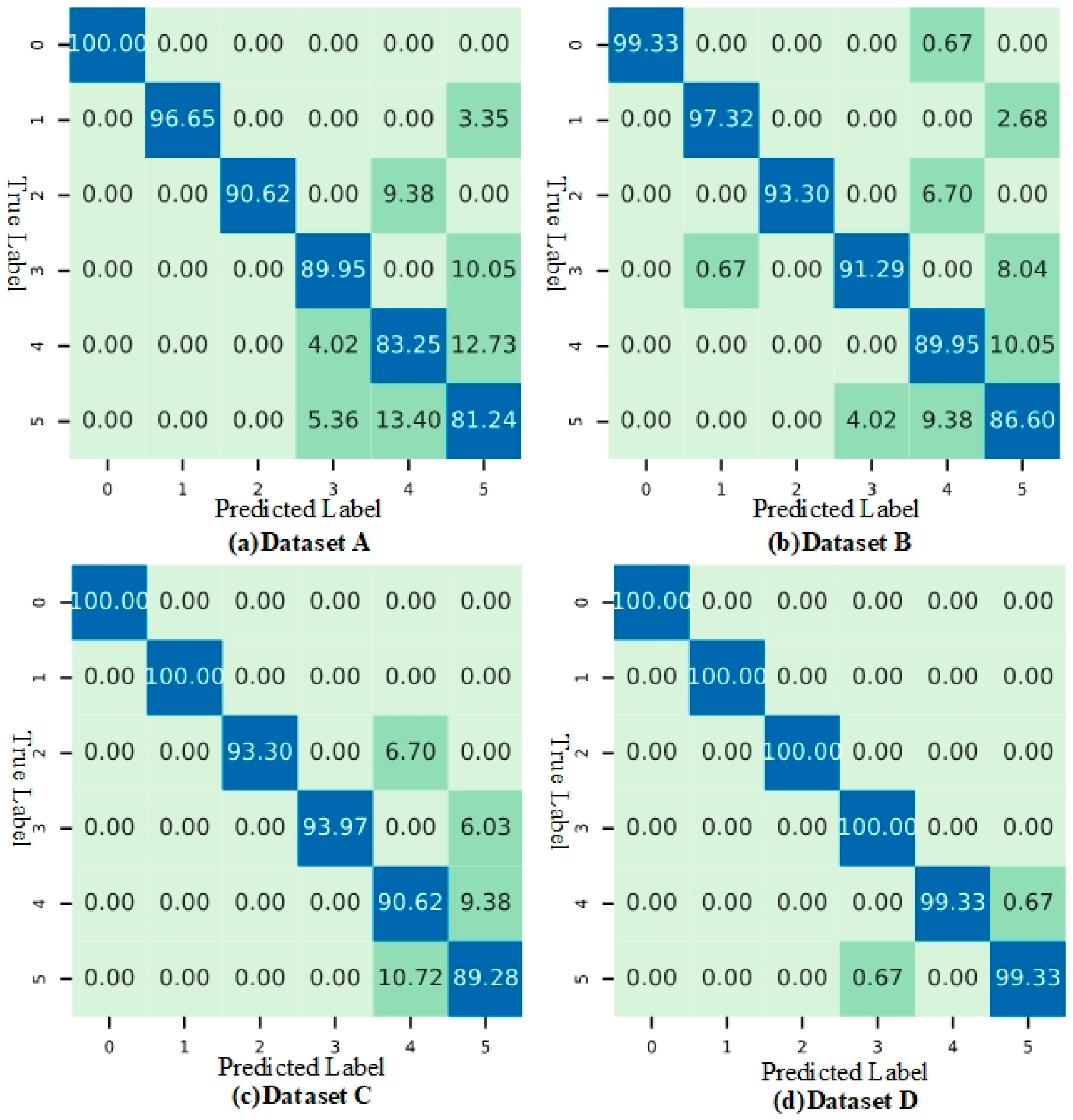
PU Dataset: Four imbalanced sample datasets are designed, named Dataset A, Dataset B, Dataset C, and Dataset D. Each dataset has a different imbalance ratio range, and the calculation method is as follows:

$$p=\left[{\displaystyle \frac{Number of samples of the leastfault type}{Number of normal samples}},{\displaystyle \frac{Number of samples of the most fault type}{Number of normal samples}}\right]$$

(14)

As the value of P decreases, the degree of imbalance in the dataset increases. The ratio of the number of samples between the most and least fault categories is set to 3:1. For example, Dataset A has the highest degree of imbalance, with 15 samples for fault type KA03 and 5 samples for fault type KI03. Therefore, the imbalance ratio range for Dataset A is $\left[0.01,0.03\right]$.To better evaluate the overall performance of the model, the test set is a balanced dataset, with 150 samples for normal and each fault category, totaling 900 samples. The detailed information of the PU dataset is shown in

Table 3. Details of the PU datasets.

Dataset	Number of Classes	Normal Sample Number	Fault Class Sample Number					p
		K001	KA03	KA05	KA07	KI01	KI03
A	6	500	15	12	9	7	5	0.01–0.03
B	6	500	30	23	15	14	10	0.02–0.06
C	6	500	75	61	52	29	25	0.05–0.15
D	6	500	150	130	106	70	50	0.1–0.3

.

(2)

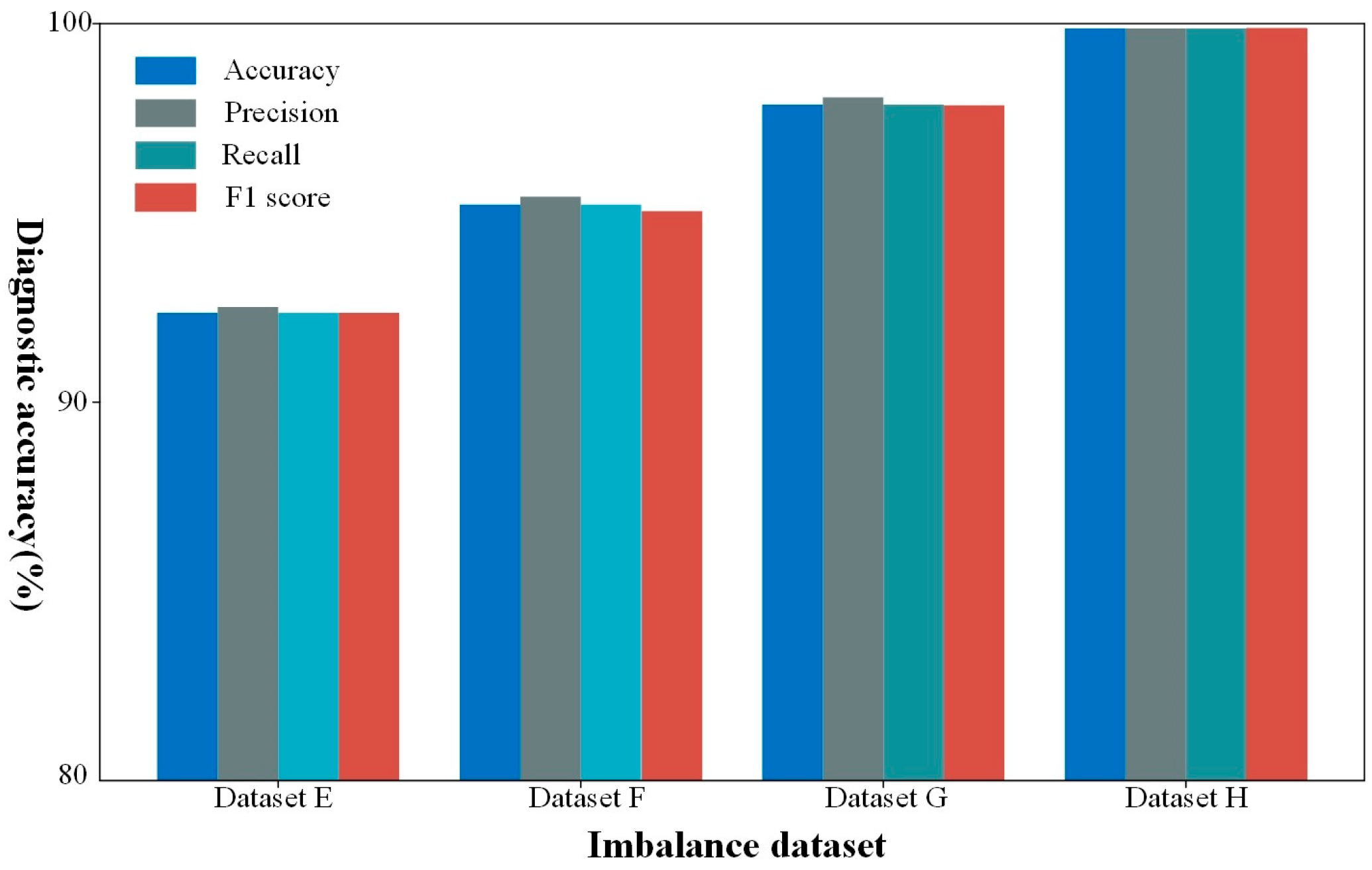
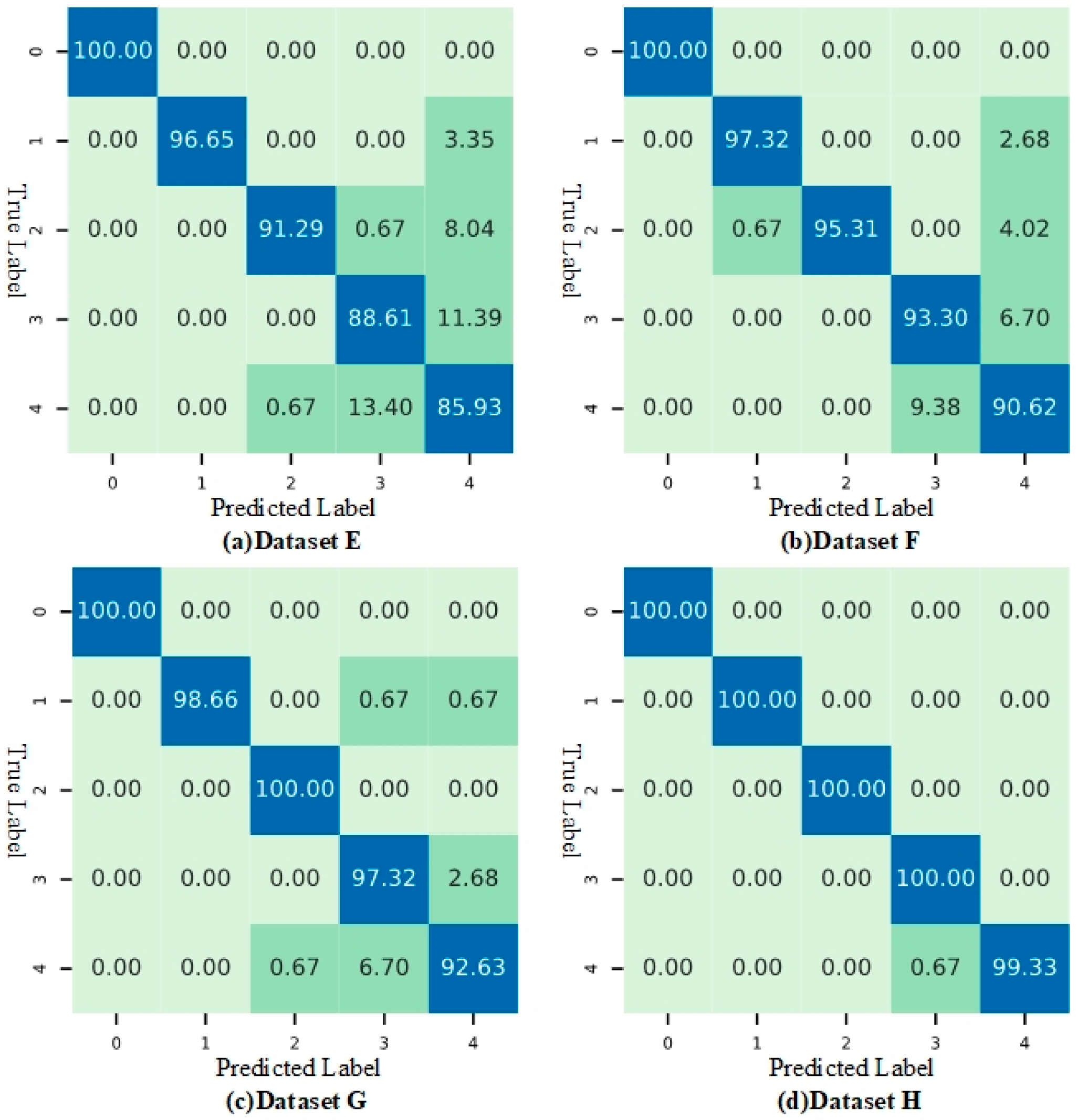
HUST Dataset: Similarly, four imbalanced sample datasets are designed, named Dataset E, Dataset F, Dataset G, and Dataset H. Each dataset has a different imbalance ratio range, and the ratio of the number of samples between the most and least fault categories is set to 2:1. For example, Dataset E has the highest degree of imbalance, with the number of samples for fault category O being the most at 8 and for fault category C being the least at 4. According to Equation (14), the imbalance ratio range for Dataset E is $\left[0.008,0.016\right]$. The test set is set as a balanced dataset, with 150 samples for normal and each fault category, totaling 750 samples. The detailed information of the HUST dataset is shown in

Table 4. Details of the HUST datasets.

Dataset	Number of Classes	Normal Sample Number	Fault Class Sample Number				p
		N	O	I	B	C
E	5	480	8	6	5	4	0.008–0.016
F	5	480	12	11	9	6	0.0125–0.025
G	5	480	40	33	27	20	0.042–0.083
H	5	480	96	82	65	48	0.1–0.2

.

3.3. Paderborn University Bearing Experiment

This section will evaluate the fault diagnosis performance of the proposed method using the Paderborn University bearing dataset, compares different data generation methods and assesses the effectiveness of various network models.

3.3.1. Analysis of Fault Diagnosis Performance

To comprehensively validate the effectiveness of the proposed method, the test set data were used to evaluate models trained on the four datasets. The test set is balanced, with 150 samples for normal and each fault category, totaling 900 samples. Four evaluation metrics—accuracy, precision, recall, and F1 score—were utilized to comprehensively measure the diagnostic performance of the model when dealing with imbalanced datasets. During the experiments, we first applied the KDE-ADASYN method to augment the samples in each dataset, achieving class balance. Next, we used the FFT technique to transform the time-domain signals into frequency-domain representations. The signals were then normalized to standardize their amplitude and eliminate any inconsistencies due to sensor characteristics. Finally, the preprocessed data were fed into the 1D-MobileNet network integrated with the SE block for training and evaluation. To ensure the reliability of the results, we conducted the experiments 10 times and averaged the metrics to obtain the final results.

Table 5. Details of the PU datasets after applying KDE-ADASYN.

Dataset	Number of Classes	Normal Sample Number	Fault Class Sample Number					p
		K001	KA03	KA05	KA07	KI01	KI03
A	6	500	105	84	63	49	35	0.07–0.21
B	6	500	210	161	105	98	70	0.14–0.42
C	6	500	500	427	364	203	175	0.35–1.0
D	6	500	500	500	500	490	350	0.7–1.0

presents the details of the PU dataset after applying the KDE-ADASYN method to augment samples. Compared with Table 3, the results clearly show that the state of class imbalance in the dataset improved significantly.

Figure 6 shows the diagnostic effectiveness of the proposed method on each dataset. As shown in the figure, the proposed method exhibits outstanding diagnostic performance across various imbalanced datasets. In Dataset D, which has the least imbalance, the method achieved over 99% accuracy, precision, recall, and F1 score, demonstrating exceptionally strong classification performance. Although diagnostic performance decreases as the degree of imbalance increases, it remains high. Even in the extremely imbalanced Dataset A, the method achieved around 90% in accuracy, precision, recall, and F1 score. This fully demonstrates that the method has excellent fault diagnosis capabilities under various imbalance ratio fluctuations, indicating its applicability to real-world scenarios.

To better illustrate the method’s fault identification capabilities across various imbalanced datasets, we present the confusion matrix in Figure 7. The predicted labels 0, 1, 2, 3, 4, and 5 in Figure 7 correspond to K001, KA03, KA05, KA07, KI01, and KI03, respectively. The matrix demonstrates that the method performs exceptionally well in identifying faults in moderately imbalanced datasets, such as Datasets C and D, with accuracy rates exceeding 94%. However, in highly imbalanced datasets like Dataset A, while the overall diagnostic accuracy decreases slightly, the metrics below 90% are primarily concentrated in labels 4 and 5, while the recognition accuracy for labels 1 and 2 remains relatively high.

3.3.2. Comparison of Different Data Generation Methods

To verify the superior performance of the proposed method in data generation, multiple methods were designed for comparison, and a detailed comparative analysis was conducted with the method proposed in this paper.

(1)

BEGSMOTE: The boundary enhancement and Gaussian mixture model optimized synthetic minority oversampling technique (BEGSMOTE) method combines boundary enhancement (BE) and the Gaussian mixture model (GMM) to optimize the synthetic minority oversampling technique. This method aims to overcome the sample density insufficiency problem in traditional SMOTE models while addressing the limitations of deep learning models in terms of training sample size and processing speed [20]. This technique was used to balance the dataset samples, followed by applying FFT transformation to the sample signals to obtain frequency-domain signal data. Finally, the data were trained and evaluated using a 1D-MobileNet network integrated with the SE block. The comparison results of each method with the method proposed in this paper are shown in

Table 6. Comparative results of different generation methods.

Dataset	Method	Acc (%)	P (%)	R (%)	F1 (%)
A	BEGSMOTE	86.69	86.84	86.69	86.60
	ADASYN	84.42	84.61	84.42	84.40
	GAN	88.17	88.32	88.17	88.23
	Proposed method	90.38	90.12	89.64	89.60
B	BEGSMOTE	88.52	88.71	88.52	88.49
	ADASYN	87.61	87.79	87.61	87.57
	GAN	91.73	91.87	91.73	91.70
	Proposed method	93.02	93.19	93.03	93.01
C	BEGSMOTE	89.96	90.14	89.96	89.94
	ADASYN	88.42	88.62	88.42	88.46
	GAN	92.61	92.78	92.61	92.60
	Proposed method	94.58	94.79	94.58	94.58
D	BEGSMOTE	96.93	97.15	96.93	96.90
	ADASYN	95.02	95.23	95.02	94.98
	GAN	98.83	99.02	98.83	98.81
	Proposed method	99.73	99.68	99.63	99.61

.

(2)

ADASYN: Adaptive synthetic sampling (ADASYN) is an oversampling technique that uses a weighted distribution to calculate the density of surrounding samples, taking into account the varying learning difficulties of minority class samples. ADASYN generates more synthetic data for minority class samples that are harder to learn compared to those that are easier to learn. The same evaluation steps were applied to this technique as to BEGSMOTE.

(3)

GAN: The generative adversarial network (GAN) learns the data distribution of the minority class through a generator and generates new samples to address data imbalance issues [38]. This method first converts the sample signals from the time domain to the frequency domain using FFT. Then, GAN is used to generate training data to balance the samples. The data were input into a 1D-MobileNet network, which was integrated with the SE block, for training and evaluation.

As shown in Table 6, when the degree of imbalance in the dataset is low, such as in Dataset D, the quality of fault samples extended by the three methods is relatively high, resulting in diagnostic accuracy rates over 95% for the models. As the degree of imbalance increases, the quality of the samples generated by the three methods decreases, leading to varying declines in the diagnostic accuracy of the models. Among them, the samples generated by GAN have a distribution relatively consistent with real samples, so the diagnostic accuracy can still be maintained above 90%. When the fault sample data are severely imbalanced, such as in Dataset A, the quality of samples generated by all three methods is hard to guarantee. In comparison, the diagnostic accuracy of the model using the proposed method can still reach 90%. Notably, the proposed method consistently maintains significant superiority across various imbalance ratio fluctuation ranges, demonstrating excellent boundary decision capabilities. This indicates that the method is fully applicable for monitoring equipment in real industrial scenarios.

3.3.3. Comparison of Different Network Models

To verify the effectiveness and computational performance of the network model, multiple deep learning network models were selected for comparison, as shown in

Table 7. Description of the different model structures.

Network	Description	Primary Characteristics
1D-CNN	One-dimensional convolutional neural network	One-dimensional standard convolutional neural network
1D-CNN-G [39]	One-dimensional CNN with GAP	Network with standard convolutional kernel and maximum pooling in the first layer and a global average pooling layer in the last layer
1D-ResNet	One-dimensional ResNet	One-dimensional standard residual network
1D-ShuffleNet	One-dimensional ShuffleNet	By adopting channel shuffle and group convolution, the computational cost and the number of parameters is reduced
Inception-v2 [40]	Improved inception architecture	Reduced computational cost and memory usage through factorized convolutions and streamlined operations

.

To emphasize the comparison of computational performance, we select the relatively balanced Dataset D for the experiment, with the results presented in

Table 8. Comparison between different methods using Dataset D.

	Parameter Count	Memory Usage (MB)	Inference Time (s)	Acc (%)
1D-ResNet	36,913	0.1408	2.78	98.84
1D-CNN-G	32,156	0.1227	2.51	98.51
1D-CNN	16,983	0.0648	2.04	98.78
Inception-v2	28,038	0.107	2.38	98.83
1D-ShuffleNet	14,829	0.0566	1.83	99.21
Proposed method	2992	0.0114	1.01	99.72

. For a fair comparison, consistent preprocessing steps are applied across all network models. Specifically, KDE-ADASYN is first used to augment the dataset and achieve class balance. Next, FFT is applied to transform the time-domain signals into frequency-domain representations. The signals are then normalized to standardize their amplitude and eliminate any inconsistencies due to sensor characteristics. Finally, the preprocessed data are fed into the various network models for training and evaluation. Under conditions of relatively balanced sample data, all six methods achieve high diagnostic accuracy; however, our proposed method demonstrates clear advantages. In terms of model parameters and memory usage, the proposed method requires only about one-sixth of the parameters and memory usage of the standard 1D-CNN and one-eleventh of those in 1D-CNN-G. Regarding computational performance, our method also outperforms the others in inference time, reducing it by 1.03 s compared to 1D-CNN and 1.5 s compared to 1D-CNN-G. While Inception-v2 is effective at capturing multi-scale features, our approach offers significant advantages. It uses only about one-tenth of the parameters and memory usage of Inception-v2, reduces inference time by 1.37 s, and achieves higher prediction accuracy. In conclusion, the proposed method substantially reduces network parameters, memory usage, and computational resource consumption, while maintaining superior accuracy. These advantages make it particularly well suited for real-time monitoring of mobile industrial equipment.

3.4. Huazhong University of Science and Technology Bearing Experiment

This section will evaluate the fault diagnosis performance of the proposed method using the Huazhong University of Science and Technology bearing dataset and compare different data generation methods.

3.4.1. Analysis of Fault Diagnosis Performance

To further verify the effectiveness and generalization performance of the proposed method, the model was trained using the imbalanced datasets E, F, G, and H from Huazhong University of Science and Technology and its performance was evaluated using the test set.

Table 9. Details of the HUST datasets after applying KDE-ADASYN.

Dataset	Number of Classes	Normal Sample Number	Fault Class Sample Number				p
		N	O	I	B	C
E	5	480	56	42	35	28	0.056–0.112
F	5	480	84	77	63	42	0.0875–0.175
G	5	480	280	231	189	140	0.292–0.583
H	5	480	480	480	455	336	0.7–1.0

provides the details of the HUST dataset after applying the KDE-ADASYN method for sample augmentation. Compared to Table 4, the results clearly demonstrate a significant improvement in addressing class imbalance within the dataset.

As illustrated in Figure 8, the evaluation metrics for all datasets exceed 90%, with Datasets F and G achieving metrics above 95%, and Dataset H’s metrics nearing 100%.This result once again fully confirms the effectiveness and applicability of the proposed method. More importantly, compared to the results from the PU experiments, the diagnostic performance in the HUST experiments is even more outstanding. We speculate that this might be related to the different ratio settings between the most and least fault categories in the two experiments. This finding validates that the degree of imbalance among minority classes, i.e., fault categories, also significantly impacts classifier performance, further confirming the research value of the issues raised in this paper.

The confusion matrices in Figure 9 demonstrate the performance of the proposed method across Datasets E, F, G, and H. For the extremely imbalanced Dataset E, the method primarily exhibited classification errors between labels 3 and 4, while maintaining high recognition accuracy for other categories. As the sample imbalance decreases, misclassification between categories gradually diminishes. In Datasets F, G, and H, the recognition accuracy for each category exceeds 95%, with the highest surpassing 99%, highlighting the method’s exceptional fault diagnosis capabilities and robust generalization ability.

3.4.2. Comparison of Different Data Generation Methods

Similar to previous comparisons, the method proposed in this paper was compared with BEGSMOTE, ADASYN, and GAN to verify its applicability in different experimental scenarios. The diagnostic results of each method on different datasets are shown in

Table 10. Comparative results of different generation methods.

Dataset	Method	Acc (%)	P (%)	R (%)	F1 (%)
E	BEGSMOTE	89.14	89.35	89.14	89.13
	ADASYN	87.39	87.60	87.39	87.38
	GAN	90.25	90.42	90.25	90.24
	Proposed method	92.36	92.51	92.36	92.36
F	BEGSMOTE	92.33	92.53	92.33	92.32
	ADASYN-	91.41	91.60	91.41	91.41
	GAN	93.73	93.90	9373	93.72
	Proposed method	95.22	95.43	95.22	95.21
G	BEGSMOTE	95.71	95.90	95.71	95.70
	ADASYN	95.12	95.21	95.12	95.12
	GAN	96.59	96.79	96.59	96.58
	Proposed method	97.86	98.05	97.86	97.84
H	BEGSMOTE	97.94	98.14	97.94	97.94
	ADASYN	97.72	97.91	97.72	97.70
	GAN	98.97	99.18	98.97	98.97
	Proposed method	99.88	99.87	99.86	99.86

. As seen, when the degree of imbalance is low, such as in Dataset H, all methods perform well, with the GAN slightly outperforming BEGSMOTE and ADASYN. As the sample imbalance becomes more severe, the diagnostic performance of all methods decreases. However, the proposed method still achieves 92% accuracy in the extremely imbalanced Dataset E and attains the highest performance metrics on each dataset. This once again demonstrates its significant advantages and broad applicability in addressing issues across various imbalance ratio fluctuation ranges.

4. Conclusions

To address the challenges of data imbalance in real-world engineering and the complexity of applying neural networks in real-time monitoring, this study introduces a lightweight fault diagnosis model for mechanical equipment based on MobileNet, enhanced with KDE-ADASYN and an SE block. The KDE-ADASYN algorithm adaptively generates fault samples to balance the data, while FFT converts time-domain signals into frequency-domain signals. The integration of the SE block further enhances the model’s fault feature recognition capabilities. In fault simulation experiments, four metrics—accuracy, precision, recall, and F1 score—were employed to thoroughly evaluate the diagnostic performance on various imbalanced datasets. The results demonstrated that the proposed method consistently delivers excellent performance. Additionally, the validation process explored the necessity of each component in the method, with comparative experiments confirming that the proposed approach achieved optimal performance across all metrics, while also reducing network parameters and minimizing computational resource consumption.

In future work, we aim to address several key challenges: First, we will tackle the issues encountered in real-world scenarios, where data typically contain higher levels of noise, more diverse operating conditions, and complex fault scenarios that were not fully captured in this study. Second, we plan to explore the model’s ability to generalize across different experimental setups, devices, and operating conditions. Finally, we will investigate multi-modal approaches, integrating vibration data with other sensor modalities (e.g., acoustic or thermal data) to enhance the model’s performance and robustness.

References

1. Zhou, P.; Chen, S.; He, Q.; Wang, D.; Peng, Z. Rotating machinery fault-induced vibration signal modulation effects: A review with mechanisms, extraction methods and applications for diagnosis. Mech. Syst. Signal Process. 2023, 200, 110489. [Google Scholar] [CrossRef]
2. Li, X.; Wang, Y.; Yao, J.; Li, M.; Gao, Z. Multi-sensor fusion fault diagnosis method of wind turbine bearing based on adaptive convergent viewable neural networks. Reliab. Eng. Syst. Saf. 2024, 245, 109980. [Google Scholar] [CrossRef]
3. Zou, Y.; Zhao, W.; Liu, T.; Zhang, X.; Shi, Y. Research on High-Speed Train Bearing Fault Diagnosis Method Based on Domain-Adversarial Transfer Learning. Appl. Sci. 2024, 14, 8666. [Google Scholar] [CrossRef]
4. Zhang, D.; Tao, H. Bearing Fault Diagnosis Based on Parameter-Optimized Variational Mode Extraction and an Improved One-Dimensional Convolutional Neural Network. Appl. Sci. 2024, 14, 3289. [Google Scholar] [CrossRef]
5. Wang, W.; Song, H.; Si, S.; Lu, W.; Cai, Z. Data augmentation based on diffusion probabilistic model for remaining useful life estimation of aero-engines. Reliab. Eng. Syst. Saf. 2024, 252, 110394. [Google Scholar] [CrossRef]
6. Ma, C.; Wang, X.; Li, Y.; Cai, Z. Broad zero-shot diagnosis for rotating machinery with untrained compound faults. Reliab. Eng. Syst. Saf. 2024, 242, 109704. [Google Scholar] [CrossRef]
7. Ma, C.; Li, Y.; Wang, X.; Cai, Z. Early fault diagnosis of rotating machinery based on composite zoom permutation entropy. Reliab. Eng. Syst. Saf. 2023, 230, 108967. [Google Scholar] [CrossRef]
8. Yin, W.; Xia, H.; Huang, X.; Wang, Z. A fault diagnosis method for nuclear power plants rotating machinery based on deep learning under imbalanced samples. Ann. Nucl. Energy 2024, 199, 110340. [Google Scholar] [CrossRef]
9. Wan, W.; Chen, J.; Xie, J. Graph-Based Model Compression for HSR Bogies Fault Diagnosis at IoT Edge via Adversarial Knowledge Distillation. IEEE Trans. Intell. Transp. Syst. 2023, 25, 1787–1796. [Google Scholar] [CrossRef]
10. Han, T.; Liu, C.; Wu, L.; Sarkar, S.; Jiang, D. An adaptive spatiotemporal feature learning approach for fault diagnosis in complex systems. Mech. Syst. Signal Process. 2019, 117, 170–187. [Google Scholar] [CrossRef]
11. Dorneanu, B.; Zhang, S.; Ruan, H.; Heshmat, M.; Chen, R.; Vassiliadis, V.S.; Arellano-Garcia, H. Big data and machine learning: A roadmap towards smart plants. Front. Eng. Manag. 2022, 9, 623–639. [Google Scholar] [CrossRef]
12. Gong, W.; Chen, H.; Zhang, Z.; Zhang, M.; Wang, R.; Guan, C.; Wang, Q. A novel deep learning method for intelligent fault diagnosis of rotating machinery based on improved CNN-SVM and multichannel data fusion. Sensors 2019, 19, 1693. [Google Scholar] [CrossRef] [PubMed]
13. Liu, Y.; Yan, X.; Zhang, C.; Liu, W. An ensemble convolutional neural networks for bearing fault diagnosis using multi-sensor data. Sensors 2019, 19, 5300. [Google Scholar] [CrossRef] [PubMed]
14. Li, H.; Liu, F.; Kong, X.; Zhang, J.; Jiang, Z.; Mao, Z. Knowledge features enhanced intelligent fault detection with progressive adaptive sparse attention learning for high-power diesel engine. Meas. Sci. Technol. 2023, 34, 105906. [Google Scholar] [CrossRef]
15. Tong, Q.; Lu, F.; Feng, Z.; Wan, Q.; An, G.; Cao, J.; Guo, T. A Novel Method for Fault Diagnosis of Bearings with Small and Imbalanced Data Based on Generative Adversarial Networks. Appl. Sci. 2022, 12, 7346. [Google Scholar] [CrossRef]
16. Liu, Z.; Liu, J.; Huang, Y.; Li, T.; Nie, C.; Xia, Y.; Zhan, L.; Tang, Z.; Zhang, L. Fault critical point prediction method of nuclear gate valve with small samples based on characteristic analysis of operation. Materials 2022, 15, 757. [Google Scholar] [CrossRef]
17. Wang, R.; Zhang, S.; Chen, Z.; Li, W. Enhanced generative adversarial network for extremely imbalanced fault diagnosis of rotating machine. Measurement 2021, 180, 109467. [Google Scholar] [CrossRef]
18. Rivera, W.A. Noise reduction a priori synthetic over-sampling for class imbalanced data sets. Inf. Sci. 2017, 408, 146–161. [Google Scholar] [CrossRef]
19. Swana, E.F.; Doorsamy, W.; Bokoro, P. Tomek link and SMOTE approaches for machine fault classification with an imbalanced dataset. Sensors 2022, 22, 3246. [Google Scholar] [CrossRef]
20. Wang, Z.; Liu, T.; Wu, X.; Liu, C. A diagnosis method for imbalanced bearing data based on improved SMOTE model combined with CNN-AM. J. Comput. Des. Eng. 2023, 10, 1930–1940. [Google Scholar] [CrossRef]
21. Liang, X.; Jiang, A.; Li, T.; Xue, Y.; Wang, G. LR-SMOTE—An improved unbalanced data set oversampling based on K-means and SVM. Knowl.-Based Syst. 2020, 196, 105845. [Google Scholar] [CrossRef]
22. Han, H.; Wang, W.Y.; Mao, B.H. Borderline-SMOTE: A new over-sampling method in imbalanced data sets learning. Lect. Notes Comput. Sci. 2005, 3644, 878–887. [Google Scholar]
23. He, H.; Bai, Y.; Garcia, E.A.; Li, S. ADASYN: Adaptive synthetic sampling approach for imbalanced learning. In Proceedings of the 2008 IEEE International Joint Conference on Neural Networks, Hong Kong, China, 1–8 June 2008; pp. 1322–1328. [Google Scholar]
24. Liu, D.; Zhong, S.; Lin, L.; Zhao, M.; Fu, X.; Liu, X. Highly imbalanced fault diagnosis of gas turbines via clustering-based downsampling and deep siamese self-attention network. Adv. Eng. Inform. 2022, 54, 101725. [Google Scholar] [CrossRef]
25. Mao, G.; Li, Y.; Cai, Z.; Qiao, B.; Jia, S. Transferable dynamic enhanced cost-sensitive network for cross-domain intelligent diagnosis of rotating machinery under imbalanced datasets. Eng. Appl. Artif. Intell. 2023, 125, 106670. [Google Scholar] [CrossRef]
26. Tang, B.; He, H. KernelADASYN: Kernel-based adaptive synthetic data generation for imbalanced learning. In Proceedings of the 2015 IEEE Congress on Evolutionary Computation (CEC), Sendai, Japan, 25–28 May 2015. [Google Scholar]
27. Kurniawati, Y.E.; Permanasari, A.E.; Fauziati, S. Adaptive Synthetic–Nominal (ADASYN–N) and Adaptive Synthetic–KNN (ADASYN-KNN) for multiclass imbalance learning on laboratory test data. In Proceedings of the 2018 4th International Conference on Science and Technology (ICST), Yogyakarta, Indonesia, 7–8 August 2018. [Google Scholar]
28. Li, J.; Liu, Y.; Li, Q. Intelligent fault diagnosis of rolling bearings under imbalanced data conditions using attention-based deep learning method. Measurement 2022, 189, 110500. [Google Scholar] [CrossRef]
29. Gu, Y.; Chen, R.; Wu, K.; Huang, P.; Qiu, G. A variable-speed-condition bearing fault diagnosis methodology with recurrence plot coding and MobileNet-v3 model. Rev. Sci. Instrum. 2023, 94, 034710. [Google Scholar] [CrossRef]
30. Iandola, F.N.; Moskewicz, M.W.; Ashraf, K.; Han, S.; Dally, W.J.; Keutzer, K. SqueezeNet: AlexNet-level accuracy with 50x fewer parameters and <1 MB model size. arXiv 2016, arXiv:1602.07360. [Google Scholar]
31. Zhang, X.; Zhou, X.; Lin, M.; Sun, J. ShuffleNet: An extremely efficient convolutional neural network for mobile devices. In Proceedings of the IEEE Conference on Computer Vision and Pattern Recognition, Honolulu, HI, USA, 21–26 July 2017; pp. 6848–6856. [Google Scholar]
32. Howard, A.G.; Zhu, M.; Chen, B.; Kalenichenko, D.; Wang, W.; Weyand, T.; Andreetto, M.; Adam, H. MobileNets: Efficient convolutional neural networks for mobile vision applications. arXiv 2017, arXiv:1704.04861. [Google Scholar]
33. Yu, W.; Lv, P. An end-to-end intelligent fault diagnosis application for rolling bearing based on MobileNet. IEEE Access 2021, 9, 41925–41933. [Google Scholar] [CrossRef]
34. Landi, E.; Spinelli, F.; Intravaia, M.; Mugnaini, M.; Fort, A.; Bianchini, M.; Corradini, B.T.; Scarselli, F.; Tanfoni, M. A MobileNet neural network model for fault diagnosis in roller bearings. In Proceedings of the 2023 IEEE International Instrumentation and Measurement Technology Conference (I2MTC), Kuala Lumpur, Malaysia, 22–25 May 2023. [Google Scholar]
35. Xu, Y.; Jiang, X. Short-term power load forecasting based on BiGRU-Attention-SENet model. Energy Sources Part A Recovery Util. Environ. Eff. 2022, 44, 973–985. [Google Scholar] [CrossRef]
36. Kaiser, L.; Gomez, A.N.; Chollet, F. Depthwise separable convolutions for neural machine translation. arXiv 2017, arXiv:1706.03059. [Google Scholar]
37. Zhao, C.; Zio, E.; Shen, W. Domain generalization for cross-domain fault diagnosis: An application-oriented perspective and a benchmark study. Reliab. Eng. Syst. Saf. 2024, 245, 109964. [Google Scholar] [CrossRef]
38. Zhang, W.; Li, X.; Jia, X.; Ma, H.; Luo, Z.; Li, X. Machinery fault diagnosis with imbalanced data using deep generative adversarial networks. Measurement 2019, 152, 107377. [Google Scholar] [CrossRef]
39. Zhu, F.; Liu, C.; Yang, J. An improved MobileNet network with wavelet energy and global average pooling for rotating machinery fault diagnosis. Sensors 2022, 22, 4427. [Google Scholar] [CrossRef]
40. Szegedy, C.; Vanhoucke, V.; Ioffe, S.; Shlens, J.; Wojna, Z. Rethinking the inception architecture for computer vision. In Proceedings of the IEEE Conference on Computer Vision and Pattern Recognition, Las Vegas, NV, USA, 26 June–1 July 2016; pp. 2818–2826. [Google Scholar]
Figure 1. The KAMS fault diagnosis framework.
Applsci 14 11910 g001
Figure 2. The structure of 1D-SENet network.
Applsci 14 11910 g002
Figure 3. The structure of 1D depthwise separable convolution.
Applsci 14 11910 g003
Figure 4. The structure of 1D-MobileNet network integrated with the SE block.
Applsci 14 11910 g004
Figure 5. Test rig of HUST bearing dataset.
Applsci 14 11910 g005
Figure 6. Diagnosis results of the proposed method on PU datasets.
Applsci 14 11910 g006
Figure 7. Confusion matrix of the proposed method on PU datasets.
Applsci 14 11910 g007
Figure 8. Diagnosis results of the proposed method on HUST datasets.
Applsci 14 11910 g008
Figure 9. Confusion matrix of the proposed method on HUST datasets.
Applsci 14 11910 g009