A Robot Error Prediction and Compensation Method Using Joint Weights Optimization Within Configuration Space

Abstract

With the growing demand for industrial robots in the aerospace manufacturing process, the lack of positioning accuracy has become a critical factor limiting their broad application in precision manufacturing. To enhance robot positioning accuracy, one crucial approach is to analyze the distribution patterns of robot errors and leverage spatial similarity for error prediction and compensation. However, existing methods in Cartesian space struggle to achieve accurate error estimation when the robot is loaded or the end-effector orientations are varied. To address these challenges, a novel method for robot error prediction and accuracy compensation within configuration space is proposed. The analysis of robot error distribution reveals that the spatial similarity of robot errors is more pronounced and stable in configuration space compared to Cartesian space, and this property exhibits significant anisotropy across joint dimensions. A spatial-interpolation-based unbiased estimation method with joint weights optimization is proposed for robot errors prediction, and the particle filter method is utilized to search for the optimal joint weights, enhancing the anisotropic characteristics of the prediction model. Based on the robot error prediction model, a cyclic searching method is employed to directly compensate for the joint angles. An experimental system is established using an industrial robot equipped with a 120 kg end-effector and a laser tracker. Eighty sampling points with diverse poses are randomly selected within the task workspace to measure the robot errors before and after compensation. The proposed method achieves an error prediction accuracy of 0.172 mm, reducing the robot error from the original 4.96 mm to 0.28 mm, thus meeting the stringent accuracy requirements for hole machining in robotic aerospace assembly processes.

1. Introduction

Industrial robots with serial multi-joints are widely applied in aerospace manufacturing, undertaking tasks such as robotic welding, grinding, and hole-making. However, the lack of positioning accuracy limits their uses in high-precision machining and assembly processes. With a positional accuracy requirement of ±0.5 mm for assembly holes in aerospace components, which is significantly higher than the original accuracy of robots, error prediction and accuracy compensation methods for robots are essential.

Robot position accuracy, which refers to the consistency between the theoretical and actual position within any position and posture, is influenced by various factors, including manufacturing errors of the robot, drive errors caused by actuators and encoders, deformations in robot joints and links due to external loads and gravity, backlash in gearboxes, and temperature fluctuations. Robot errors can be categorized into geometric errors and non-geometric errors, each with different distributions and modeling methods. Kinematic models, which describe the mathematical relationship between the joint angles of a robot and its geometric state theoretically, are the primary means for analyzing geometric errors. The D-H model simplifies the parameterization of the geometric relationship between robot joints and links [1], making it commonly used, despite its incomplete parameters and singularities. To address the incompleteness in the D-H model, Hayati proposed the M-DH model, which includes additional joint geometric parameters [2]. Additionally, to overcome the singularity problems inherent in various D-H models, the Product of Exponentials (POE) formula is frequently used in the construction of robot kinematic models [3]. Distortions in the kinematic model parameters causing robot geometric errors are a major factor affecting robot positioning accuracy, and accurate identification of kinematic parameters can significantly improve robot accuracy [4,5]. The prediction and compensation of non-geometric errors, caused by factors such as structural deformations, joint backlash, or temperature changes, are also key methods to further enhance robot accuracy. Qi and Alam et al. considered the influence of elastic deformation in robot joints and links and bidirectional backlash of joints, introducing various non-geometric parameters to extend the kinematic model, and achieved precise prediction of robot positioning errors through accurate parameter identification [6,7]. Chen et al. considered the influence of both geometric and non-geometric factors on positioning errors simultaneously, establishing a rigid–flexible coupled robot error prediction model, which was further applied to trajectory accuracy compensation in robots [8]. In the prediction of robot errors, Bai et al. separated geometric and non-geometric factors, establishing both an M-DH error model and a non-geometric error model based on LSSVR, and conducted parameter identification for each model separately [9]. For scenarios where robots carry heavy loads or experience significant load changes such as robotic casting or continuous milling, Deng et al. developed joint stiffness models for the robots and predicted real-time deformation states during robot motion by utilizing joint torques either from robot joints feedback or predicted by kinematic equations, thereby achieving real-time position compensation during the robot’s movement [10,11,12,13]. The aforementioned modeling approaches aim to analyze the true mapping process between configuration space and Cartesian space theoretically. However, this process is influenced by various geometric and non-geometric factors which pose challenges to modeling, and the error evolution mechanisms of some non-geometric factors are difficult to describe. Therefore, neural-network-based methods for predicting non-geometric errors have gradually been adopted. Multilayer neural networks are utilized to simulate the distribution patterns of robot errors and dynamic status, thereby enhancing robot positioning accuracy without the need to establish dynamic equations. Zhang and Wang et al. separately established RNN and MLP models to predict structural deformations and positioning errors caused by gravity, inertia forces, and other external forces, and applied robot compensation within the offline programming process [14,15]. Peng and Liao et al., on the other hand, utilized real-time feedback information from the robot, including joint positions, velocities, and torques, to build robot compliance deformation prediction models based on CNN and RVM architectures, achieving the online prediction of robot errors [16,17].

Another approach to enhance robot accuracy is to achieve robot error prediction utilizing a set of calibration points based on the robot error spatial similarity, without the complex error models. Zeng et al. analyzed the robot error evolution mechanism of the D-H error model, proposing that the geometric robot errors exhibit spatial similarity in Cartesian space, and achieved robot error prediction using calibration points distributed in uniform grids [18]. Jiao et al. experimentally validated the spatial similarity of the robot stiffness characteristics in Cartesian space and proposed a gridded variable stiffness model to predict the non-geometric errors of the robot [19]. Using the error data of the uniform gridded points in Cartesian space, Cao and Cai et al. separately implemented robot error prediction by employing the Inverse Distance Weighting (IDW) method and Kriging method [20,21]. Neural network models constructed based on architectures such as the MLP, ELM, and RBF are also widely used in robot errors prediction [22,23,24,25], although these methods often require a large number of data from grid-sampled points. Xu and Chen et al., respectively, proposed the SSA–Elman model and the OP-ELM model for processing the error data of grid points, improving the training efficiency and accuracy of the robot error prediction model through optimized training methods [26,27]. According to the continuity of the robot motion process, Zhang and Tan et al. proposed the similarity of robot positioning errors in continuous spatiotemporal domains and combined historical data from the robot motion process to establish neural network models, achieving real-time prediction of robot positioning errors [28,29]. The aforementioned methods clearly analyze the distribution patterns and compensation principles of robot errors in Cartesian space. However, considering the serial rotary joint structure of industrial robots, utilizing joint angles to describe and control the robot status in configuration space is a more direct approach. Li et al. used surface reconstruction methods to fit the two-dimensional manifold of the robot error distribution in configuration space, revealing that the distribution of robot errors shows significant continuity in configuration space [30]. Zeng and Guo et al. demonstrated through theoretical analysis and experimental results that both geometric and non-geometric robot errors show significant spatial similarity in configuration space, and prediction models of robot errors were achieved based on spatial-interpolation-based unbiased estimation methods [31,32]. However, there is still a lack of analysis on the anisotropic distribution characteristics of the robot errors spatial similarity in configuration space. Additionally, existing error prediction methods that rely on the spatial similarity of robot errors still face challenges when the robot moves with changes in posture.

This study analyzes the spatial similarity distribution patterns of robot errors under different loads and poses in both configuration space and Cartesian space, highlighting the advantages of using joint angles to predict robot errors in configuration space. Furthermore, an anisotropic spatial-interpolation-based unbiased estimation method with joint weights optimization is proposed for robot error prediction, and a cyclic reverse search method is employed to directly compensate for the joint angles. This approach achieves effective improvements in the positioning accuracy of industrial robots when they are carrying significant loads and experiencing substantial posture changes during movement. Throughout the rest of this paper, Section 2 analyzes the different distribution patterns of the robot error spatial similarity in both configuration space and Cartesian space, and proposes a uniform sampling method for the robot task workspace in configuration space. A robot error prediction method is introduced in Section 3, along with the optimal search for joint weights and a method for compensating the robot joint angles. In Section 4, error prediction and compensation experiments based on a robot and laser tracker are conducted, and the experimental results are analyzed. The conclusion is presented in Section 5.

2. Spatial Similarity Analysis and Sampling Method of Robot Errors in Configuration Space

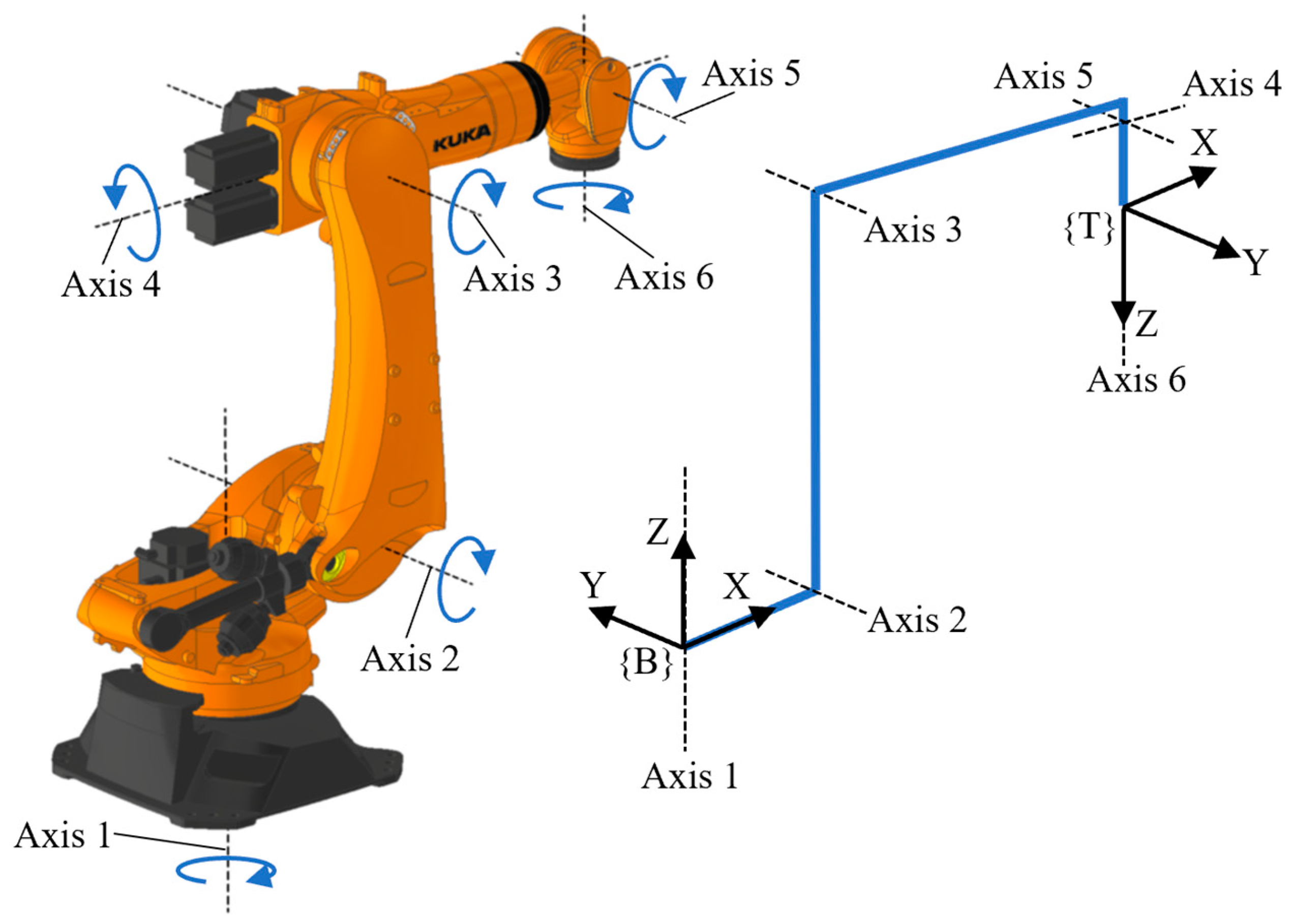
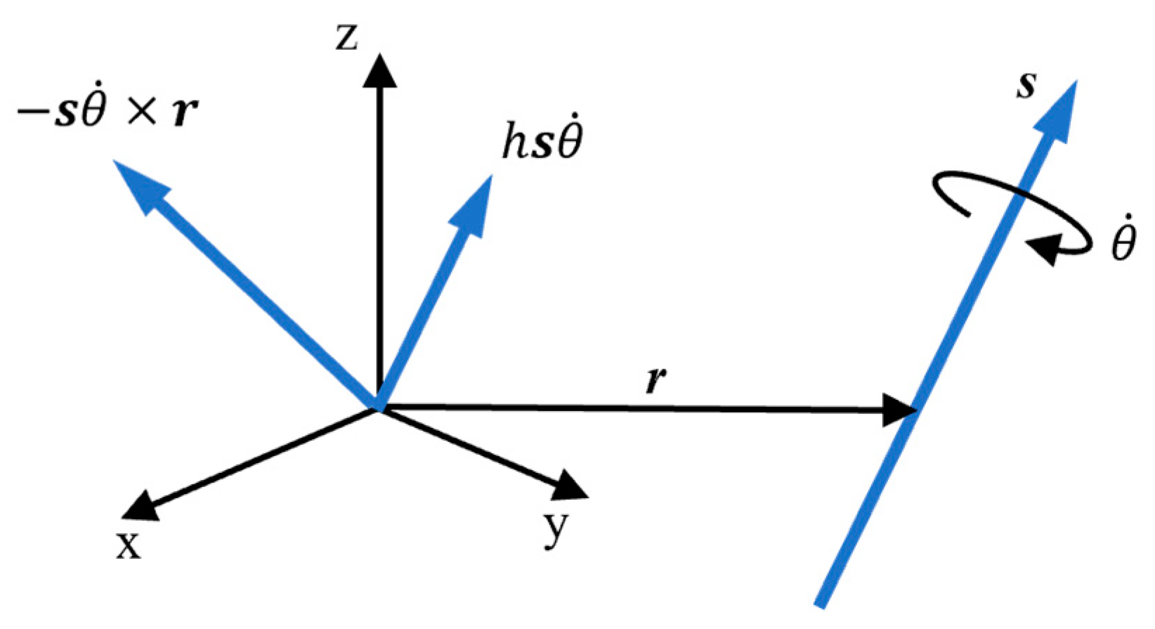
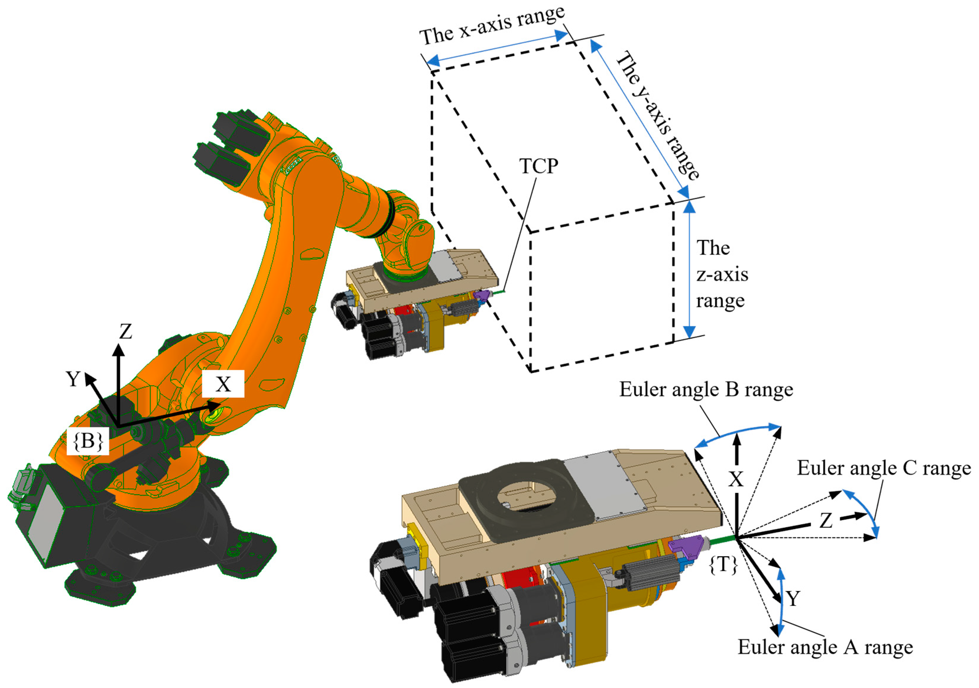
2.1. Robot Kinematics Model Construction

To investigate the distribution of industrial robot positioning errors, the base coordinate frame {B} and the tool coordinate frame {T} are firstly defined. As shown in Figure 1, the base coordinate frame of a six-axis robot is fixed to the robot base, with its Z-axis coinciding with the A1 axis of the robot, and its X-axis being perpendicular to both the A1 and A2 axes; and the tool coordinate frame is fixed to the robot flange, with its Z-axis coinciding with the A6 axis of the robot, and its X-axis being perpendicular to both the A5 and A6 axes. To determine the space status T_BT of the tool coordinate frame in the base coordinate frame for any given joint angles Q = [θ₁, θ₂, θ₃, θ₄, θ₅, θ₆], a kinematic model based on the Product of Exponentials (POE) formula is established. In this model, each rotational joint of the robot can be considered as a helical motion with a fixed axis and pitch, as illustrated in Figure 2, where s denotes the unit vector along the helix axis, r is the perpendicular vector from the {B} origin to s, and h is the intercept of the helical motion. Let $\dot{\theta }$ represent the angular velocity of the helical motion and $-\mathit{s}\dot{\theta }\times \mathit{r}$ and $h\mathit{s}\dot{\theta }$ represent the linear velocities of the origin of the coordinate frame in the radial and axial directions of the helix, respectively. The helical motion can be described by the motion screw V:

$$\mathit{V}=\left[\begin{array}{c}\mathit{\omega }\\ \mathit{v}\end{array}\right]=\left[\begin{array}{c}\mathit{s}\dot{\theta }\\ -\mathit{s}\dot{\theta }\times \mathit{r}+h\mathit{s}\dot{\theta }\end{array}\right],\mathit{V}\in {\mathbb{R}}^6$$

(1)

In analyzing the theoretical motion screws of the rotational joints on the robot, it is known that ‖ω‖ ≠ 0 and h = 0. Therefore, the motion screw V can be normalized and simplified as

$$\mathit{\xi }=\mathit{V}/‖\mathit{\omega }‖=\left[\begin{array}{c}\mathit{s}\\ \mathit{v}\end{array}\right]=\left[\begin{array}{c}\mathit{s}\\ \mathit{r}\times \mathit{s}\end{array}\right],\mathit{V}\in {\mathbb{R}}^6$$

(2)

After obtaining the motion screws of all joints based on the robot geometric structure, a theoretical kinematic model of the robot can be established using the POE formula [3]:

$${\mathit{T}}_{\mathrm{B}\mathrm{T}}=F\left(\mathit{Q}\right)=e^{{\mathit{\xi }}_1{\theta }_1}{e}^{{\mathit{\xi }}_2{\theta }_2}{e}^{{\mathit{\xi }}_3{\theta }_3}{e}^{{\mathit{\xi }}_4{\theta }_4}{e}^{{\mathit{\xi }}_5{\theta }_5}{e}^{{\mathit{\xi }}_6{\theta }_6}\mathit{M}$$

(3)

where ξ_i represents the normalized motion screw of joint i, θ_i is the rotation angle of joint i, and M is the space status T_BT when all joint angles are set to 0.

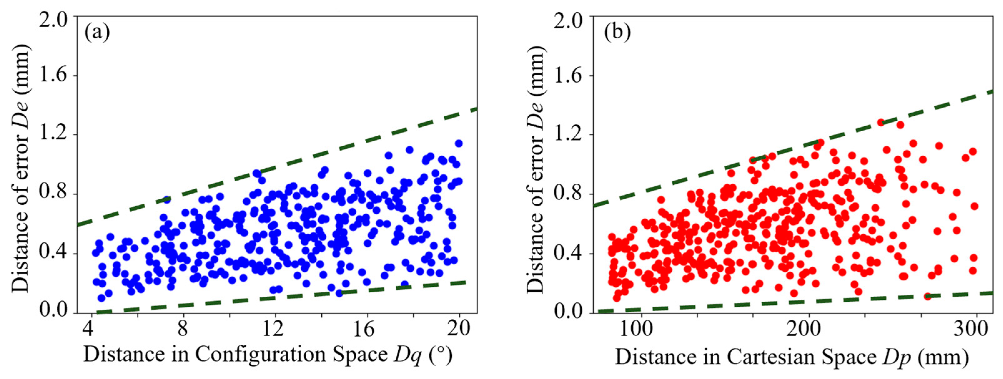
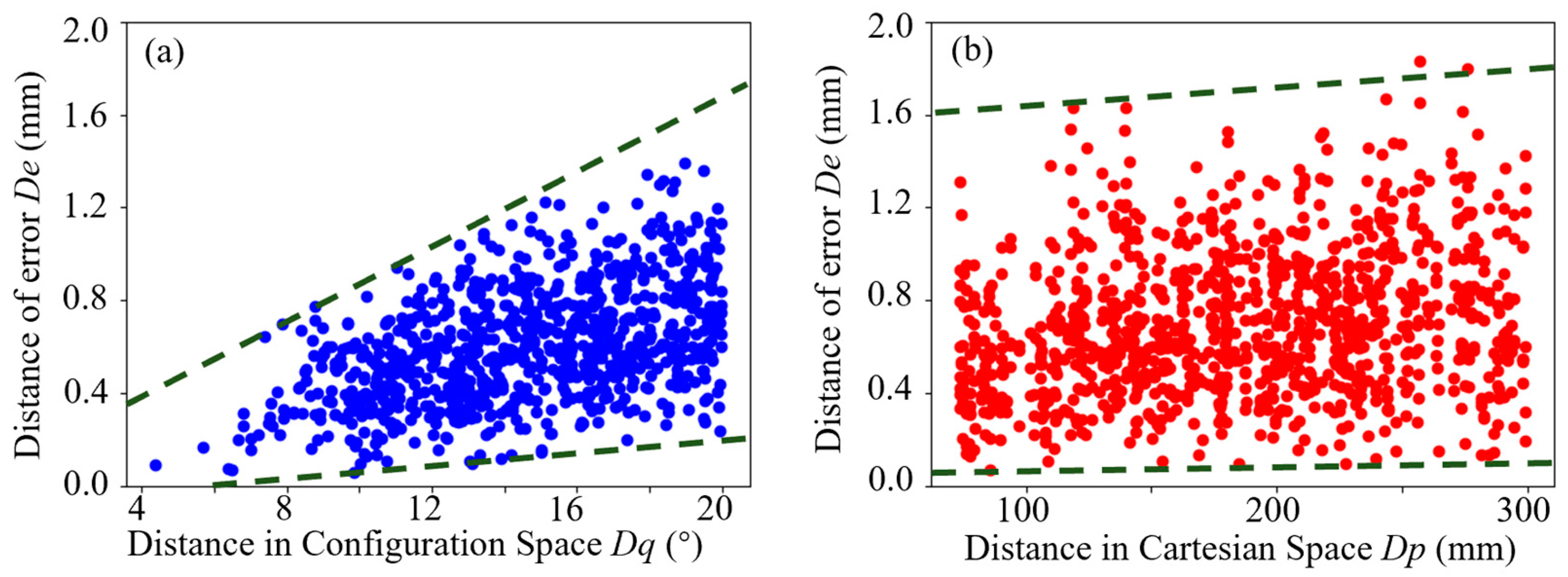
2.2. Spatial Distribution Patterns of Robot Errors in Configuration Space

In robot configuration space, the theoretical position P of the Tool Center Point (TCP) for any joint angles Q can be solved using the robot kinematic model as shown in Equation (3), denoted as P = f (Q). The robot positioning error e is defined as the inconsistency between the theoretical position and the actual position of the TCP, and the distribution function of robot errors in configuration space is defined as

$$\mathit{e}=E\left(\mathit{Q}\right)$$

(4)

According to the theoretical analysis and experimental validation by Zeng et al. [18,31], for two reachable points of the robot, whether in Cartesian space or configuration space, the smaller the distance between the two coordinates, the more similar the robot errors. This phenomenon is referred to as the spatial similarity of robot errors. Let Q₁ be the joint angles where the TCP’s theoretical position is P₁ and the corresponding positioning error is e₁ and Q₂ be the joint angles where the TCP’s theoretical position is P₂ with an error of e₂. The distance between the joint angles in the configuration space is defined as Dq = ‖Q₁ − Q₂‖, the Euclidean distance between the TCP positions is Dp = ‖P₁ − P₂‖, and the Euclidean distance between the positioning errors is De = ‖e₁ − e₂‖. In configuration space, the spatial correlation function of robot errors is defined as

$$De=g\left(Dq\right)$$

(5)

To reveal the spatial similarity of robot errors, a definition of the spatial correlation function in Equation (5) is given as

$${\displaystyle \frac{d\left(De\right)}{d\left(Dq\right)}}={\displaystyle \frac{\nabla ‖E\left({\mathit{Q}}_1\right)-E\left({\mathit{Q}}_2\right)‖}{\nabla ‖{\mathit{Q}}_1-{\mathit{Q}}_2‖}}={\displaystyle \frac{De}{Dq}}{\displaystyle \frac{(E\left({\mathit{Q}}_1\right)-E({\mathit{Q}}_2\left)\right)(dE\left({\mathit{Q}}_1\right)-dE({\mathit{Q}}_2\left)\right)}{{(\mathit{Q}}_1-{\mathit{Q}}_2\left)\right({d\mathit{Q}}_1-{d\mathit{Q}}_2)}}$$

(6)

Due to the continuous differential manifold of robot positioning errors in the configuration space [30], the error distribution function will be sufficiently smooth and exhibit local monotonic properties similar to those in Euclidean space when the distance Dp between Q₁ and Q₂ is sufficiently small. At this point, the differential function of the spatial correlation shown in Equation (6) is always positive, which means that the robot errors exhibit significant spatial similarity within any local region in the configuration space. Meanwhile, in Cartesian space, the spatial correlation function of robot positioning errors is defined as

$$De=h\left(Dp\right)$$

(7)

And a definition of the spatial correlation function in Cartesian space as shown in Equation (7) is given as

$${\displaystyle \frac{d\left(De\right)}{d\left(Dp\right)}}={\displaystyle \frac{\nabla ‖{\mathit{e}}_1-{\mathit{e}}_2‖}{\nabla ‖{\mathit{P}}_1-{\mathit{P}}_2‖}}$$

(8)

Although any reachable joint angles of a six-DOF robot correspond to a unique TCP position according to the kinematic model shown in Equation (3), solving for the joint angles corresponding to any given TCP position is a multi-solution problem due to the redundant degrees of freedom. Only when the robot end-effector orientation is fixed does the TCP position correspond to a unique set of joint angles, and only under this condition can Equation (8) be expressed as

$${\displaystyle \frac{d\left(De\right)}{d\left(Dp\right)}}={\displaystyle \frac{\nabla ‖{\mathit{e}}_1-{\mathit{e}}_2‖}{\nabla ‖{\mathit{P}}_1-{\mathit{P}}_2‖}}={\displaystyle \frac{\nabla ‖E\left({\mathit{Q}}_1\right)-E\left({\mathit{Q}}_2\right)‖}{\nabla ‖f\left({\mathit{Q}}_1\right)-f\left({\mathit{Q}}_2\right)‖}}$$

(9)

At this point, in Cartesian space, the distribution pattern of robot errors shows significant spatial similarity. However, Equation (8) will no longer hold if the orientation of the robot end-effector changes, and the spatial similarity of robot errors in Cartesian space exhibits pronounced singularity.

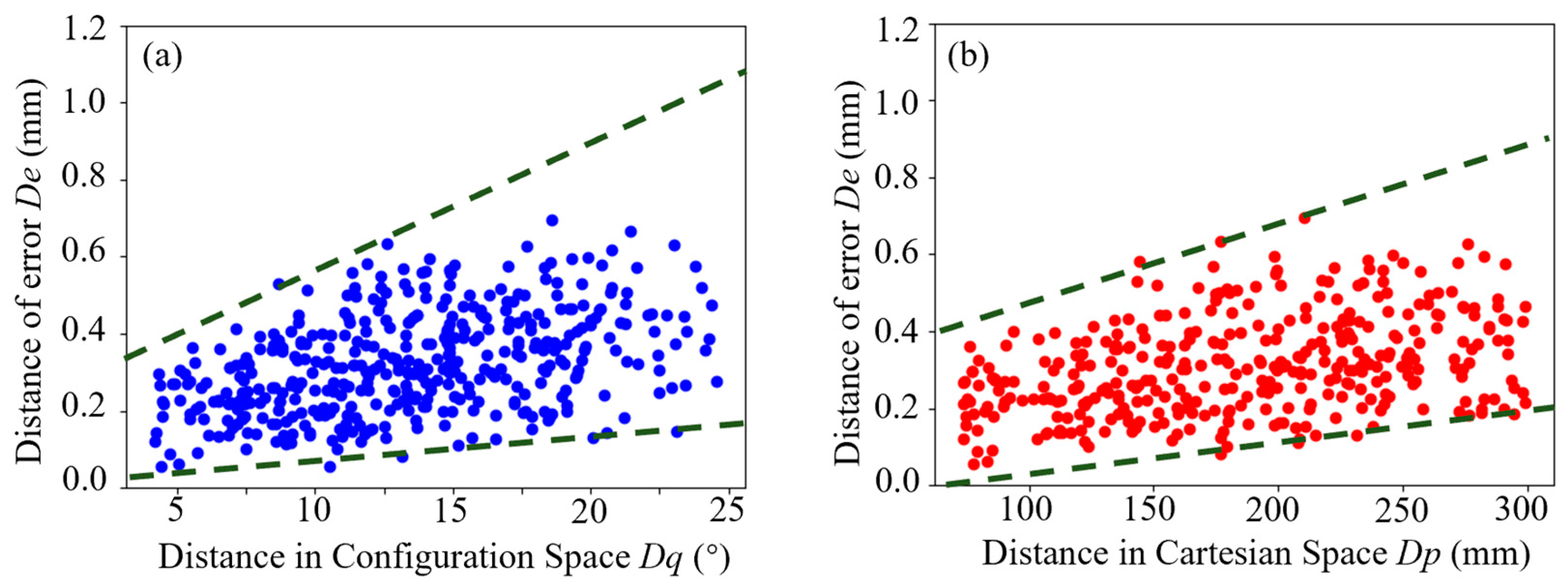
2.3. Experimental Analysis of Robot Error Spatial Similarity in Configuration Space

A measurement system is set up to verify the spatial similarity distribution characteristics of robot errors, as shown in Figure 3, and a series of comparative experiments is conducted. A KUKA KR300 R2500-ultra robot (KUKA AG, Augsburg, Germany) equipped with a hole-making end-effector with a weight of 120 kg is used and an FARO Vantage-E6 laser tracker (FARO Technologies Inc., Orlando, FL, USA) is employed to measure the real TCP positions of the end-effector. During the experiments, the spatial similarity distribution of robot errors is verified under two conditions: when the robot is unloaded or loaded and when the end-effector orientation is fixed or changed. A 1.5 inch Spherical Mounted Retroreflector (SMR) (FARO Technologies Inc., Orlando, FL, USA) is mounted on the end of the robot, with its center defined as the TCP.

Before the experiment, the base coordinate system {B} and tool coordinate system {T} of the robot are measured and calculated using the laser tracker. In the measurement of {B}, the A1 and A2 axes are rotated sequentially, and the trajectories of the TCP are measured using the laser tracker. Then, the Z-axis of the {B} system is defined, aligning with the A1 axis, and the X-axis is defined perpendicular to both the A1 and A2 axes, based on the coordinate system definition shown in Figure 1. In the measurement of {T}, the A5 and A6 axes are rotated sequentially, and the trajectories of the TCP are measured and the rotation axes are calculated. The X-axis of the {T} system is defined, aligning with the A6 axis, the Z-axis is defined perpendicular to both the A5 and A6 axes, and the SMR center is defined as the TCP.

A rectangular region of 1 m × 1 m × 0.5 m is selected within the robot task workspace for experimental measurement of the robot error distribution in Cartesian space, and 50 points are randomly chosen within this region, with robot end-effector orientations fixed. A range of joint angles is also selected for experimental measurement of the robot error distribution in configuration space with the following ranges: A1 Range = [−5°, 5°], A2 Range = [−85°, −95°], A3 Range = [85°, 95°], A4 Range = [−5°, 5°], A5 Range = [85°, 95°], A6 Range = [−5°, 5°]. Fifty joint angles are randomly selected as the measurement set within this sampling space, ensuring that the robot end-effector orientations are varied. The load status of the robot is considered in two scenarios: unloaded and under 120 kg load. During the experiment, depending on whether the robot pose is fixed or varied, a sample point list of the fixed or varying pose is selected, and the robot is controlled to move to each position sequentially for the real TCP position measurement. After the measurements, for each sampling point, the theoretical TCP position is calculated based on the joint angles using Equation (3), and the robot error is then determined as the difference between the theoretical TCP position and the real TCP position. The spatial similarity of robot errors is analyzed based on the measurement data in both configuration space and Cartesian space.

In the scenario where the robot is unloaded and the pose is fixed, the spatial correlation of robot errors in configuration space can be represented by the distribution of De on Dq, as shown in Equation (5), and the scatter plot of De on Dq is illustrated in Figure 4a. When Dq is small, the value of De is also small, with a tightly clustered distribution, indicating that, when the joint angles between two points are close in configuration space, the robot errors are also similar. As Dq increases, De also increases significantly, with a more dispersed distribution, indicating that, when the joint angles differ greatly in configuration space, the positioning errors also differ significantly. Meanwhile, with the robot unloaded and the pose fixed, the spatial correlation of robot errors in Cartesian space can be represented by the distribution of De on Dp, as shown in Equation (7), and the scatter plot of De on Dp is illustrated in Figure 4b. As Dp increases gradually, De also increases from small values, with the distribution becoming more dispersed. In the comparison between Figure 4a,b, it can be observed that, with the robot unloaded and pose fixed, the spatial similarity of robot errors is significant in both configuration space and Cartesian space, consistent with the trends shown in Equations (6) and (9).

For the scenario where the robot is unloaded and the pose varies, the scatter plot of De on Dq is shown in Figure 5a. When Dq is small, De is also small and the distribution is tightly clustered. As Dq increases, De also increases significantly, and the distribution becomes more dispersed. The scatter plot of De on Dp is shown in Figure 5b, showing that changes in Dp have a smaller impact on De, and the distribution of De remains uniform but dispersed. Clearly, when the robot is unloaded and the pose varies, the spatial similarity of robot errors remains significant in configuration space but is not as apparent in Cartesian space.

For the scenario where the robot is under a 120 kg load and the pose is fixed, the scatter plot of De on Dq is shown in Figure 6a, and the scatter plot of De on Dp is shown in Figure 6b. As Dq or Dp gradually increases, De shows a gradual increase, with a distribution that is more dispersed. Clearly, under these conditions, the spatial similarity of robot positioning errors is significant in both configuration space and Cartesian space. However, it is also observed that, compared to the scenario where the robot unloaded and the pose fixed, when the robot is under a heavy load, De is higher at the same distances, indicating a noticeable decrease in the robot accuracy.

For the scenario where the robot is under a 120 kg load and the pose varies, the scatter plot of De on Dq is shown in Figure 7a. As Dq gradually increases, De also increases significantly, and the distribution becomes more dispersed. The scatter plot of De on Dp is shown in Figure 7b, showing that changes in Dp make little impact on De, and the distribution is uniform and dispersed, indicating that changes in Dp have a minimal effect on De. Clearly, when the robot has a heavy load and the pose varies, significant error spatial similarity can still be observed in configuration space, while this characteristic almost disappears in Cartesian space.

To quantitatively analyze the distribution characteristics of robot error similarity in Cartesian space and configuration space, the correlation between error similarity and spatial distance for different measurement samples is calculated utilizing the Pearson Correlation Coefficient (PCC), which is a statistical method to analyze the correlation between continuous variables [33]. The PCC between the error similarity and spatial distance for a set of points can be calculated as follows [34]:

$$\mathrm{P}\mathrm{C}\mathrm{C}={\displaystyle \frac{cov\left(\right\{De\},\{D\left\}\right)}{std\left(\right\{De\left\}\right)·std\left(\right\{D\left\}\right)}},\mathrm{P}\mathrm{C}\mathrm{C}\in [-\mathrm{1,1}]$$

(10)

where {De} is the set of error distances between any two points in the measurement set, and {D} represents the set of distances between any two points. When analyzing the error spatial similarity in configuration space, each element in {D} is the Dq between every two sampling points, while, in Cartesian space, each element in {D} is the Dp of sampling points. When the PCC between two sets of variables is positive, a higher PCC value indicates a stronger positive correlation; when the PCC value approaches 0, the correlation between the two variables sets is almost non-existent.

The PCC values between the positioning errors De and the joint angle distance Dq for different robot load and pose conditions in configuration space are shown in

Table 1. PCC between the error similarity and distance among sampling points in configuration space.

Load Status	Pose Variation Status	PCC	p-Value
0 kg	Pose fixed	0.469	1.236 × 10−22
120 kg	Pose fixed	0.424	3.498 × 10−12
0 kg	Pose varied	0.472	3.671 × 10−26
120 kg	Pose varied	0.403	1.261 × 10−26

. When the robot is unloaded, the PCC between the De and Dq remains above 0.4, indicating a significant spatial similarity of positioning errors, regardless of whether the pose varies or not. When the robot is under a load of 120 kg, the PCC between De and Dq decreases but still remains above 0.4. Evidently, in configuration space, the robot error spatial similarity is pronounced and stable, is unaffected by pose variations, and only slightly decreases with the increase in load.

The PCC values between the positioning errors De and the joint angle distance Dp for different robot load and pose conditions in Cartesian space are shown in

Table 2. PCC between the error similarity and distance among sampling points in Cartesian space.

Load Status	Pose Variation Status	PCC	p-Value
0 kg	Pose fixed	0.440	1.435 × 10−14
120 kg	Pose fixed	0.381	1.854 × 10−12
0 kg	Pose varied	0.214	1.021 × 10−12
120 kg	Pose varied	0.226	1.414 × 10−14

. When the end-effector pose is fixed, the PCC between the De and Dp is 0.44 while the robot is unloaded, and it decreases to 0.381 when the robot is loaded with 120 kg. However, when the robot pose varies, the PCC between the De and Dp rapidly decreases to below 0.226, regardless of whether the end-effector is loaded or not. Evidently, in Cartesian space, when the end-effector pose is fixed, the spatial similarity of robot errors remains relatively significant, although it decreases with the load; however, when the pose varies, this characteristic significantly drops to an insignificant level, regardless of the load condition.

In summary, the spatial similarity of robot errors is pronounced and stable in configuration space. Therefore, in the process of robot error prediction and accuracy compensation, it is more appropriate to directly sample the positioning errors based on the robot joint angles in configuration space and to predict the positioning errors using the sampling points.

2.4. Sampling Method of Robot Task Workspace in Configuration Space

The theoretical workspace of a robot refers to the set of all reachable space statuses in configuration space, typically described by the angle ranges that each joint can take. In the robotic aerospace manufacturing and assembly scenarios, the actual moving range of robot is constrained by factors such as the size of the end-effector, the geometric shape of the workpiece, and objects in the surrounding environment. The configuration space is divided into free space C_free where the robot can move freely and obstacle space C_obs where the robot interferes with other entities. Only in the C_free can the robot movement be planned. The robot moving range is usually further restricted based on the actual motion requirements during practical operations, which is defined as the task workspace of the robot. The task workspace is simultaneously a subset of the theoretical workspace and the C_free, and shows typical shape characteristics depending on the specific task content. Shown in Figure 8 is a typical task workspace of an aerospace hole-making robot processing a large-sized aircraft component. According to the geometric shape of the target workpiece, the TCP is confined within a rectangular prism, and the end-effector pose is limited to a fixed range based on the surface curvature and the distribution of the assembly holes. The task workspace can be respectively defined by the range of the TCP position and the range of end-effector pose variations. The range of the TCP position can be described as the value ranges along the x-axis, y-axis, and z-axis directions in the base coordinate system {B}. The range of the pose can be described using the range of the Z-Y-X Euler angles between the tool coordinate system {T} and the robot’s base coordinate system {B}, as shown in Figure 8. The angle around the Z-axis of {T} is defined as A, the angle around the Y-axis as B, and the angle around the X-axis as C. The task workspace of the robot, denoted as W_task, can be represented in Cartesian space as

$$\begin{array}{c}{\mathit{W}}_{\mathrm{t}\mathrm{a}\mathrm{s}\mathrm{k}}=\{\left(X,Y,Z,A,B,C\right)\in {\mathbb{R}}^6{\mathrm{x}}_{\mathrm{m}\mathrm{i}\mathrm{n}}\le X\le {\mathrm{x}}_{\mathrm{m}\mathrm{a}\mathrm{x}},{\mathrm{y}}_{\mathrm{m}\mathrm{i}\mathrm{n}}\le Y\le {\mathrm{y}}_{\mathrm{m}\mathrm{a}\mathrm{x}},{\mathrm{z}}_{\mathrm{m}\mathrm{i}\mathrm{n}}\le Z\le {\mathrm{z}}_{\mathrm{m}\mathrm{a}\mathrm{x}},\\ {\mathrm{A}}_{\mathrm{m}\mathrm{i}\mathrm{n}}\le A\le {\mathrm{A}}_{\mathrm{m}\mathrm{a}\mathrm{x}},{\mathrm{B}}_{\mathrm{m}\mathrm{i}\mathrm{n}}\le B\le {\mathrm{B}}_{\mathrm{m}\mathrm{a}\mathrm{x}},{\mathrm{C}}_{\mathrm{m}\mathrm{i}\mathrm{n}}\le C\le {\mathrm{C}}_{\mathrm{m}\mathrm{a}\mathrm{x}}\}\end{array}$$

(11)

To establish the robot error prediction model, it is essential to create a uniform sampling set of the robot joint angles within W_task, and the robot errors at these sampling points will be measured. However, while the W_task can be described accurately and intuitively in Cartesian space as shown in Figure 8, it is a challenge to define the W_task directly in configuration space through the range of joint angle values. Therefore, the first step is to conduct N dense samplings of W_task in Cartesian space, followed by transforming these samples into a dense set of N joint angles using the inverse kinematics model. The dense set of joint angles is then sorted by each of the six joint dimensions and uniformly partitioned into regions according to the joint angle values of the corresponding dimension. Samples are randomly taken from these regions that cover the entire W_task, ultimately obtaining a sparse sampling set S = {Q₁, Q₂, …, Q_n} with n joint angles. The complete sampling method is illustrated in Figure 9. Before establishing the error prediction model, it is necessary to measure the robot errors at each point in S.

3. Robot Error Prediction and Accuracy Compensation Method

During the sampling process of robot error distribution, the robot errors are measured at n sampling points uniformly distributed within the W_task, forming a sampling set in configuration space that includes the set of joint angles Q = {Q₁, Q₂, …, Q_n} and the corresponding set of positioning errors E = {E₁, E₂, …, E_n}. Subsequently, the robot errors prediction and joint angle compensation methods are achieved by leveraging the spatial similarity of robot errors in configuration space. In this process, the distribution characteristics of robot errors in configuration space are thoroughly exploited.

3.1. Anisotropy Analysis of Robot Positioning Error Distribution in Configuration Space

The spatial correlation of robot errors in configuration space can be represented through semivariograms based on the joint angle dataset Q and the corresponding positioning error dataset E. Furthermore, utilizing the semivariogram to establish a semivariance map, calculate the covariance vector, and solve for the error weights enables an effective approach for the unbiased estimation of robot errors at any position [20,31,32]. To achieve this objective, it is essential to first define the range of the task workspace based on the operational requirements and actual environmental constraints of the robot. According to this defined range, uniform sampling of joint angles is performed in the configuration space, following the method shown in Figure 9, and the actual robot errors at these sampled points are measured. While the task workspace defined in Cartesian space has a regular shape, its uniformly sampled joint angles in configuration space often exhibit irregular distributions. To eliminate the scale differences in the sampling points across different joints, the mean values ${\mathit{\mu }}^{joint}$, ${\mathit{\mu }}^{error}$ and the standard deviations ${\mathit{\sigma }}^{joint}$, ${\mathit{\sigma }}^{error}$ of the datasets Q and E are calculated. Then, the joint angles and positioning errors are standardized to produce ${\mathit{Q}}^{std}$ and ${\mathit{E}}^{std}$. To establish an empirical semivariogram for the standardized sampling data, the distance H between the joint angles of any two points is first calculated as

$$\mathit{H}=\left\{h_{ij}|h_{ij}=‖{\mathit{Q}}_i^{std}-{\mathit{Q}}_j^{std}‖,0\le i<j\le n\right\},\mathit{H}\in {\mathbb{R}}^{n(n-1)/2}$$

(12)

and, based on the range of values in H, 20 equally spaced intervals are set. The midpoints of these intervals are defined as h = [h₀, h₁, …, h₂₀], where h₀ = H_min and h₂₀ = H_max. The empirical semivariance value in the interval [$h_l,h_{l+1}$] of the positioning error components along the x-axis, y-axis, and z-axis is denoted as

$${\gamma }_{x,y,z}\left(h_l\right)={\displaystyle \frac{1}{2N(h_l,h_{l+1})}}{\sum }_{i,j:h_{ij}\in [h_l,h_{l+1}]}{({\mathit{e}}_{i(x,y,z)}^{std}-{\mathit{e}}_{j(x,y,z)}^{std})}^2$$

(13)

According to the semivariograms of the robot errors distributed in configuration space, as shown in Figure 10a, the semivariance at the starting point of the joint angles distance is close to zero, indicating a small nugget effect. And the semivariance gradually increases with the distance, showing that the components of positioning errors along the x-, y-, and z-axis exhibit significant spatial similarity in configuration space. However, due to the serial layout of the robot rotation joints, the six dimensions of joint angles have a notably strong correlation in the position errors of TCP. Therefore, despite the error spatial similarity observed in Cartesian space generally showing consistent distribution characteristics across the x, y, and z dimensions [18], the error spatial similarity observed in configuration space may exhibit significant anisotropy across different joint angle dimensions. To verify this hypothesis, the robot errors are separately expanded along the six joint dimensions, and the empirical semivariance distribution characteristics of the robot errors in each of the six joint dimensions are analyzed.

The semivariance distribution of the x-direction error component across the joint dimensions is shown in Figure 10b. In the A3 and A5 joint dimensions, the semivariance distribution of the x-direction error component shows a clearly better linearity with a strong positive correlation, and the nugget effect is relatively small. In contrast, the correlation between the semivariance and the joint angles distance in the other four joint dimensions is weaker, and the nugget effect at the starting point is more pronounced. Clearly, the distribution characteristics of the x-direction error component in the A3 and A5 joint dimensions exhibit more significant spatial similarity compared to those in the other four joint dimensions. As shown in Figure 10c, the semivariance distribution of the y-direction error component across the joint dimensions is unfolded. The spatial similarity of the y-direction error component is more prominent, with higher precision and consistency at distances close to zero in the A2, A6, and A1 joint dimensions compared to the A3, A4, and A5 joint dimensions. As shown in Figure 10d, the semivariance distribution of the z-direction error component across the joint dimensions is also unfolded. Clearly, the spatial similarity of the z-direction error component is more significant in the A1, A3, A4, and A5 joint dimensions, while it is less evident in the A2 and A6 dimensions, and the nugget effect is also stronger.

According to the analysis of the experimental results, although robot positioning errors exhibit significant and consistent spatial similarity in configuration space, this characteristic also shows markedly different nugget effects and sensitivities across various joint angle dimensions. Notably, the distribution of robot errors exhibits anisotropy across different joint dimensions in configuration space, which can directly impact the effectiveness of error prediction. Therefore, when constructing the error prediction model based on robot error spatial similarity, emphasis should be placed on enhancing the influence of joint dimensions with more significant spatial similarity while suppressing those with a pronounced nugget effect. This approach will improve the sensitivity of error prediction and reduce random errors.

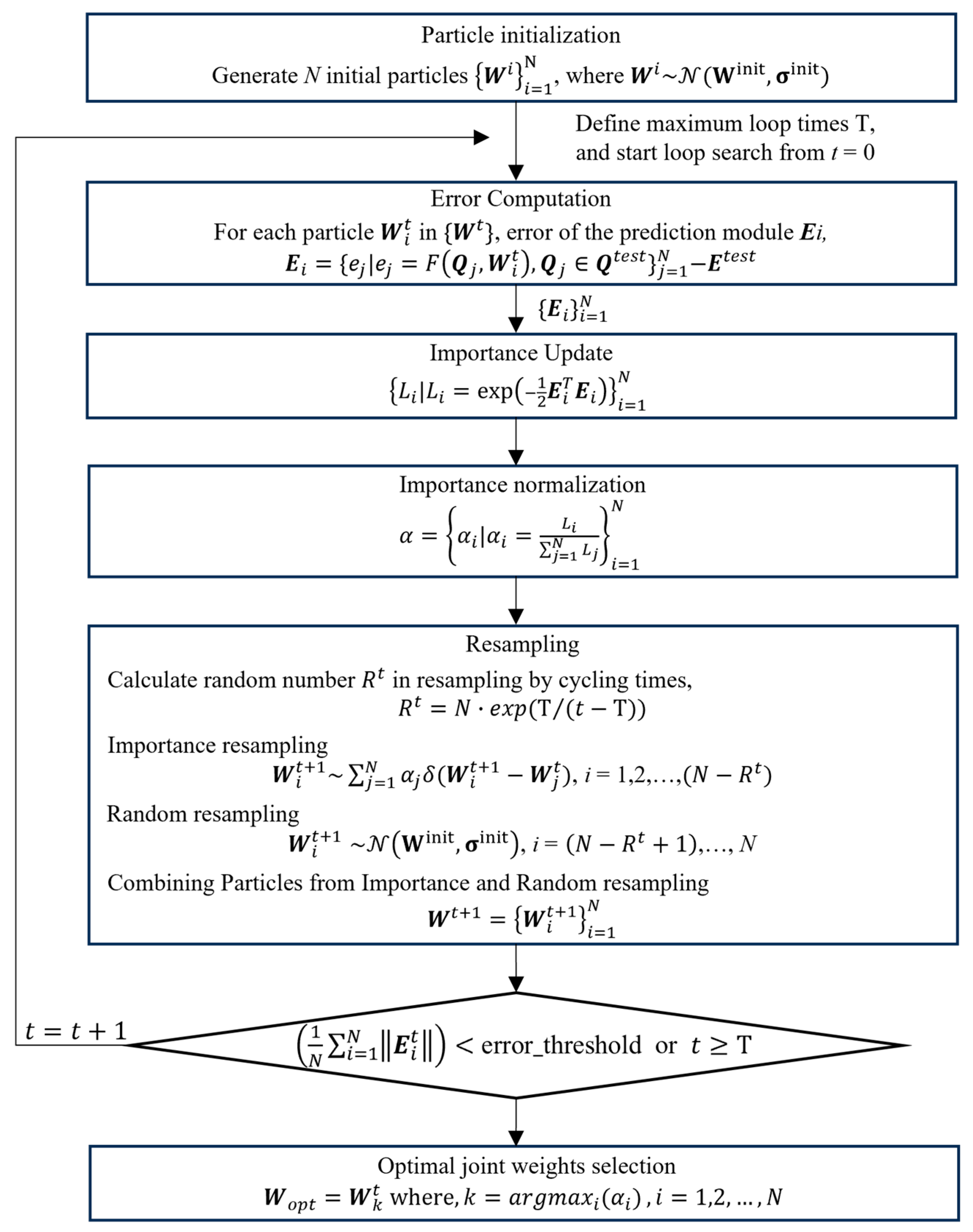
3.2. Spatial-Interpolation-Based Unbiased Error Estimation Method with Joint Weights Optimization

The x-, y-, and z-axis error components are treated as three independent features in configuration space, and, for each, a spatial-interpolation-based unbiased error estimate model is constructed. Taking the x-axis error component e_x as an example, the joint angle distances H for all elements of Q^std are first calculated and divided into equal-interval regions for semivariogram calculation, as shown in Equations (12) and (13). Then, the Gaussian semivariogram function for a distance h of any two joint angles is defined as

$$\gamma \left(h\right)=Cn+Cs(1-\exp \left(-3h^2/{Cr}^2\right)),h\in \mathit{H}$$

(14)

where Cn is the nugget effect, Cs is the sill parameter, and Cr is the range parameter. During the model training process, initial values for the semivariogram parameters Cn, Cs, and Cr are defined, and the least squares method is used to fit the semivariogram parameters by minimizing the difference between the empirical semivariance obtained from Equation (13) and the model semivariance. Then, the covariance matrix C of the sampling point errors is calculated as

$$\mathit{C}=\{C_{ij}|C_{ij}={\left({\mathit{\sigma }}^{error}\right)}^2\exp \left(-{\displaystyle \frac{3{\left(‖{\mathit{Q}}_{\mathit{i}}-{\mathit{Q}}_{\mathit{j}}‖\right)}^2}{{{\mathrm{C}}_{\mathrm{r}}}^2}}\right),0\le i,j<n\}$$

(15)

where ${\left({\mathit{\sigma }}^{error}\right)}^2$ is the variance of the robot errors distributed in configuration space.

In the error prediction process for the target joint angles Q_target, the covariance vector c between Q_target and the sampling points is first calculated as

$$\mathit{c}=\{c_i|c_i={\left({\mathit{\sigma }}^{error}\right)}^2\exp \left(-{\displaystyle \frac{3{\left(‖{\mathit{Q}}_{target}-{\mathit{Q}}_{\mathit{i}}‖\right)}^2}{{{\mathrm{C}}_{\mathrm{r}}}^2}}\right),0\le i<n\}$$

(16)

Subsequently, the unbiased estimation error weights w_error for the errors at Q_target is calculated by solving the equation

$${\mathit{w}}_{error}={(\mathit{C}+\lambda \mathit{I})}^{-1}\mathit{c}$$

(17)

Finally, the unbiased estimation value ${\mathit{e}}_x^{target}$ for the x-axis error component is obtained as follows:

$${\mathit{e}}_x^{target}={\mathit{w}}_{error}^T{\mathit{E}}_x^{std}$$

(18)

Utilizing the spatial-interpolation-based unbiased estimation method, as shown in Equations (14)–(18), separately to the x-, y-, and z-axis error components, the robot error prediction model for any target joint angles Q_target is denoted as

$${\mathit{E}}^{target}=F\left({\mathit{Q}}_{target}\right)$$

(19)

Due to the significant anisotropy in the distribution of robot errors across each joint dimension in configuration space and the notable differences among the x-, y-, and z-axis error components, the construction of the error model for each error component must consider the distribution characteristics of the error component across the six joint dimensions. This approach involves enhancing the dimensions with significant spatial similarity and weakening those with strong nugget effects that may introduce random noise, which will significantly improve the prediction accuracy of the error model. A method for unbiased estimation using configuration space interpolation with joint weights optimization is proposed to achieve higher precision in robot error prediction. Taking the calculation process of the x-axis error component estimate as an example, a set of joint weights W_x = [w₁, w₂, w₃, w₄, w₅, w₆] ∈ R⁶ is defined, and the standard joint angles Q^std are first weighted using W_x:

$${\mathit{Q}}^{weighted}={\mathit{Q}}^{std}diag\left({\mathit{W}}_x\right)$$

(20)

In this process, some dimensions of the joint angles can be amplified or reduced based on W_x to better adapt to the anisotropic distribution of positioning errors in configuration space. The selection of joint weights directly impacts the prediction accuracy of robot errors, and a particle filter method for searching the optimal joint weights is proposed, alongside the preparation of a new test dataset Q^test consisting of m sampling points and the corresponding robot error dataset E^test. During the search for optimal joint weights, the particle filter method regards the probability distribution of the optimal joint weights in configuration space as the state distribution of a six-dimensional vector particle swarm, employing a cyclic searching process based on particle importance update and resampling, as shown in Figure 11. First, an initial particle swarm containing N particles is generated, following the normal distribution defined by the initial joint weights W^init and the initial standard deviation σ^init. According to the distribution characteristics of the robot error spatial similarity across the joint dimensions described in Section 2.3, the initial joint weight for prediction of the x-axis error component is defined as Wx^init = [0.5, 0.5, 1.5, 0.5, 2.0, 0.5], while the initial joint weights of the y- and z-axis are defined as Wy^init = [1.5, 2.0, 0.5, 0.5, 0.5, 1.5] and Wz^init = [1.5, 0.5, 2.0, 1.0, 1.5, 0.5]. After the maximum number of iterations is set to T, the cyclic search for the optimal joint weights begins. In each iteration, the importance of each particle is first calculated. In this process, each particle is regarded as the current joint weights to perform joint dimension weighting on both the sample data Q^std and the test data Q^test, as shown in Equation (20). The established error prediction model as shown in Equation (18) is used to estimate the errors for Q^test, and the distance between the estimation results and E^test represents the model error E_i under the current particle W_i. The importance L_i of the current particle is then calculated based on the Gaussian distribution probability formula. After the importance of all particles in the current iteration has been updated, importance resampling is conducted, while random particles are also added to prevent the search process from becoming trapped in local optima. An error threshold is selected, and the search process is terminated if the mean error of the current particle swarm is less than the error threshold or the current number of search iterations has reached the maximum search iterations T. At this point, the particle with the minimum output error is selected as the optimal joint weight W_opt. The complete process of searching for joint weights is illustrated in Figure 11.

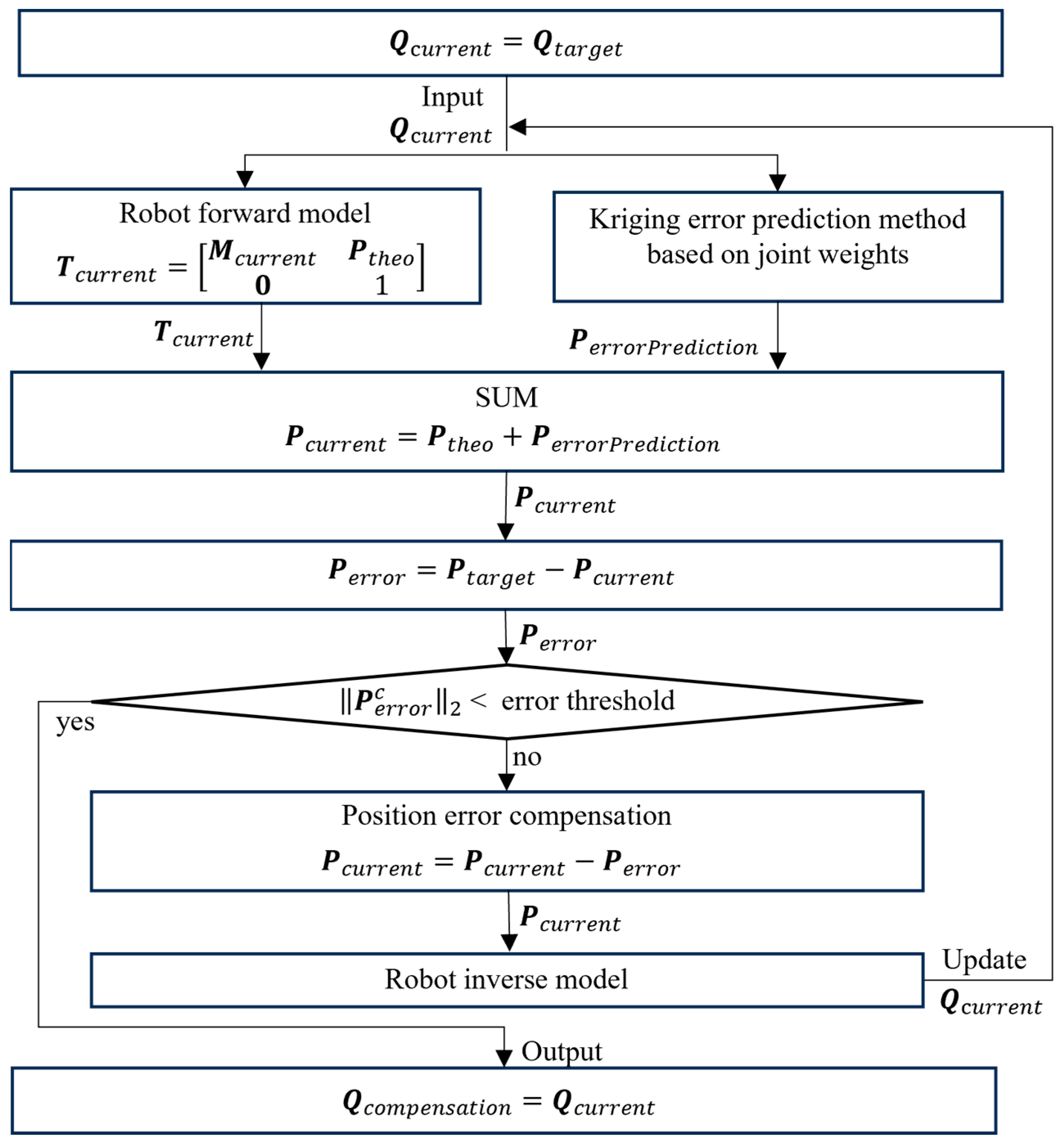
3.3. Cycling Search Method for Joint Angle Compensation

Joint angles, serving as the basic representation for describing the status of a robot in configuration space, are the most direct instructions in the programming and controlling processes of robots. Therefore, the error compensation of robot joint angles is an intuitive way to improve the robot positioning accuracy. However, while the proposed error prediction method, which utilizes the spatial similarity of robot errors, does not directly modify the parameters of the robot kinematic model, the compensated joint angles are hard to calculate through the differential equations of the kinematic model. Therefore, a joint angle compensation method based on the proposed position error prediction method that solely relies on the theoretical kinematic model is achieved, with the complete process illustrated in Figure 12. The TCP position calculated by the kinematic model from the joint angles before compensation, Q_target, serves as the target TCP position, P_target. In the iterative calculation process for joint angle compensation, the theoretical TCP position P_theo and the predicted positioning error P_{errorPrediction} corresponding to the current joint angles Q_current are first computed, and the sum is denoted as the current predicted TCP position P_current. Subsequently, the error P_error between P_target and P_current is calculated, and this error is further compensated to P_current. Finally, the inverse kinematics model is utilized to update the compensated P_current to the joint angles Q_current. The iteration stops when the magnitude of P_error is less than the error threshold, and Q_current is output as the compensated joint coordinates Q_compensation.

4. Experiments and Results

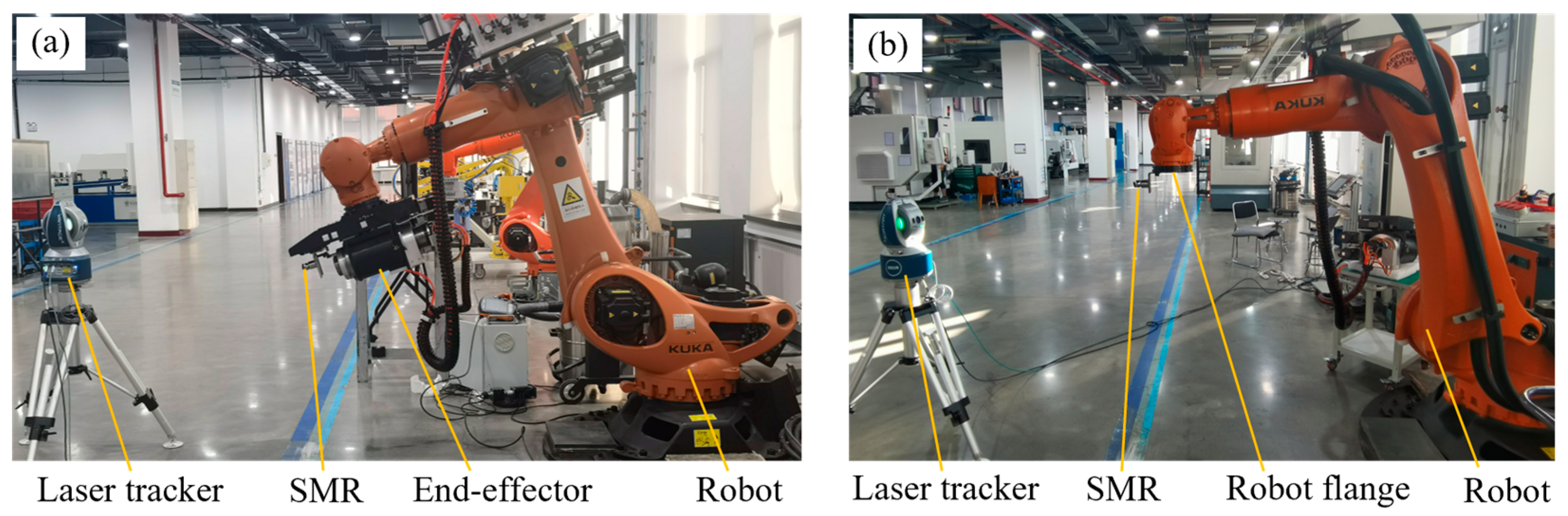
4.1. Establishment of Experimental Conditions

An experimental setup is constructed using a KUKA KR300 R2500-ultra robot equipped with a hole-making end-effector and an FARO Vantage-E6 laser tracker, to measure the robot errors and verify the accuracy of the joint angle compensation. The SMR is installed at the front of the end-effector, with its sphere center defined as the TCP. Before the start of the experiment, the robot base coordinate system {B} and the tool coordinate system {T} are calibrated, following the calibration method described in Section 2.3. Subsequently, the task workspace is defined in Cartesian space, including the TCP coordinate range in {B} and the rotation between {T} and {B}, which is defined by Z-Y-X Euler angles. Specifically, the x-axis value range of the task workspace is [1600 mm, 2400 mm], the y-axis value range is [−400 mm, 800 mm], and the z-axis value range is [−400 mm, 400 mm]. Meanwhile, the Euler angle range of A, which represents the rotation around the Z-axis, is from 85° to 95°, the Euler angle B is from 75° to 105°, and the Euler angle C is from 60° to 120°. Based on the value range of the task workspace, a set of 160 joint angle sampling points is obtained using the proposed uniform sampling method in configuration space, and the positioning errors of the robot at the sampling points are measured. Using the dataset containing 160 sampling points and positioning errors, the proposed spatial-interpolation-based unbiased estimation method with joint weights optimization is employed to establish a positioning error prediction model, and the optimal joint weights are determined based on the particle filter method. The optimal joint weights for predicting the x-axis error component are W_x = [0.985, 0.619, 1.157, 1.068, 1.216, 0.686], the optimal joint weights for the x-axis are W_y = [0.954, 1.183, 0.700, 0.667, 0.688, 1.015], and the optimal joint weights for the z-axis are W_z = [0.813, 0.349, 1.542, 0.476, 1.218, 0.353].

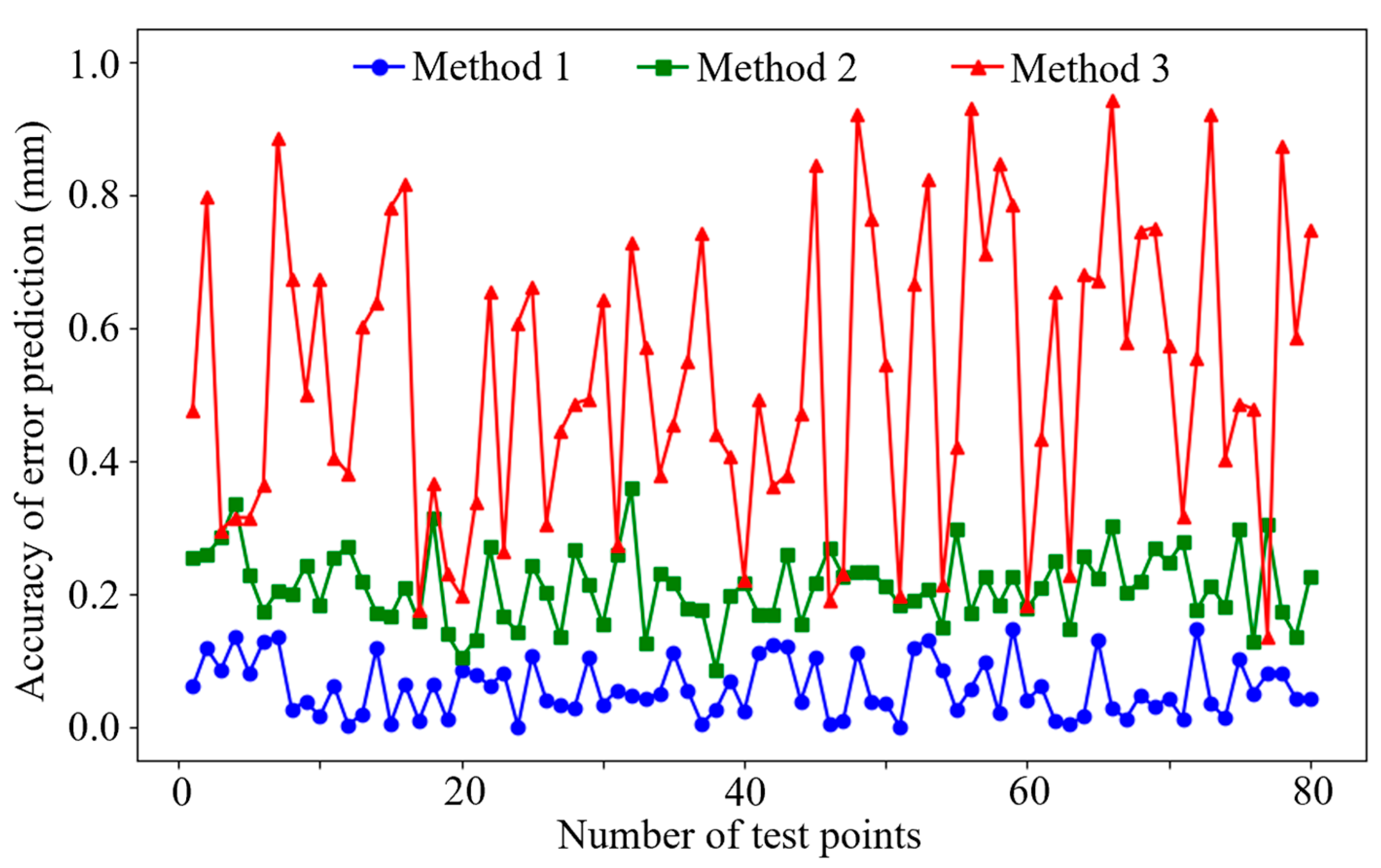
4.2. Experimental Results of Robot Error Prediction and Accuracy Compensation

In the experiments for robot error prediction and joint angle compensation, 80 groups of joint angles are randomly selected from the determined task workspace to form the test point set, and the real robot errors at these test points are measured. Among the test points, there is a significant change in the orientation of the robot end-effector. The proposed positioning error prediction method is used to estimate the positioning errors at the test points, and the distance between the estimated positioning errors and the true errors represents the accuracy of the error prediction model, as shown in Method 1 in Figure 13. Based on the proposed positioning error prediction model, after calibrating with 160 uniformly sampled data points and optimizing the joint weights using the particle filter method, the maximum error of the prediction model is less than 0.172 mm, and the average prediction error across the 80 test points is 0.089 mm. To compare the practical performance of different robot error prediction methods, other error prediction methods are reproduced, as shown in Figure 13. Method 2 utilizes an error prediction approach based on the MLP model [14] with the same sampling point set in Cartesian space, achieving a maximum prediction error of 0.359 mm and an average prediction error of 0.212 mm; Method 3 employs the spatial grid IDW algorithm for error prediction in Cartesian space [32] with the same sampling point set, resulting in a maximum error of 0.942 mm and an average error of 0.502 mm for the test point set. Results of the comparative experiment on error prediction methods are shown in

Table 3. Results of the comparative experiment on error prediction methods.

	Error Prediction Method	Average Estimated Error (mm)	Maximum Estimated Error (mm)
Method 1	The proposed method	0.089	0.172
Method 2	MLP model in Cartesian space [14]	0212	0.359
Method 3	The spatial grid IDW algorithm [32]	0.502	0.942

.

Furthermore, the 80 test points are compensated based on the proposed joint angle compensation method, obtaining the corresponding compensated joint angles. The robot is then moved to the compensated joint angles, and the positions of the compensated TCPs are measured. The distance between the compensated TCP positions and the target TCP positions is calculated, which represents the joint angle compensation accuracy. According to the experimental verification, the robot positioning error is reduced from 4.96 mm to 0.28 mm after the compensation of joint angles, as shown in Figure 14.

5. Conclusions

This study analyzed the robot error distribution in configuration space, constructed a robot error prediction model, and achieved a method for joint angle compensation. After comprehensive experimental validations, the following conclusions were drawn:

(1) A more stable and significant spatial similarity of robot errors is shown in configuration space compared to Cartesian space, especially under heavy loads and various postures.

(2) The spatial similarity of robot errors in configuration space shows marked anisotropy across different joint dimensions, and the distribution characteristics of the error components along the x-, y-, and z-axis also differ.

(3) By weighting the sampling data in configuration space using a set of joint weights, a spatial-interpolation-based unbiased estimation method with joint weights optimization can effectively address the interference caused by the anisotropy of robot error spatial similarity and accurately predict the robot errors. The optimal joint weights are selected using the particle filter method for the prediction of x, y, and z error components individually.

(4) A robot error measurement experimental system is established using a laser tracker and a six-joint industrial robot with a 120 kg end-effector. The SMR is mounted at the TCP of the end-effector for position measurement. In the error measurement experiment, 80 sampling points with diverse poses are selected within the task workspace to measure the real robot errors, thereby evaluating the accuracy of the robot error prediction model. The proposed error prediction method achieves a maximum error estimation accuracy of 0.172 mm across all sampling points, representing a 52.1% and 81.7% improvement in prediction accuracy compared to the MLP model replicated in Cartesian space and the spatial grid IDW method, respectively.

(5) In the robot position compensation experiment, the proposed method is used to adjust the joint angles of the sampling points, and the real robot errors after compensation are measured. Across all 80 sampling points, the robot error is reduced from 4.96 mm to 0.28 mm, meeting the stringent requirement for positioning accuracy in the assembly hole machining process of aerospace components. By considering the common characteristics of robot error distribution, the proposed method is applicable for enhancing the positioning accuracy of six-axis industrial robots, especially in challenging scenarios involving heavy loads and varying orientations of the end-effector.

However, the proposed method does not consider the distribution patterns or evaluation methods for the orientation errors of the robot end-effector, which will become an important direction for our future research.

References

1. Denavit, J.; Hartenberg, R.S. A Kinematic Notation for Lower-Pair Mechanisms Based on Matrices. J. Appl. Mech. 2021, 22, 215–221. [Google Scholar] [CrossRef]
2. Hayati, S.; Mirmirani, M. Improving the absolute positioning accuracy of robot manipulators. J. Robot. Syst. 1985, 2, 397–413. [Google Scholar] [CrossRef]
3. Okamura, K.; Park, F.C. Kinematic calibration using the product of exponentials formula. Robotica 1996, 14, 415–421. [Google Scholar] [CrossRef]
4. Nubiola, A.; Bonev, I.A. Absolute calibration of an ABB IRB 1600 robot using a laser tracker. Robot. Comput.-Integr. Manuf. 2013, 29, 236–245. [Google Scholar] [CrossRef]
5. Chen, G.; Wang, H.; Lin, Z. Determination of the Identifiable Parameters in Robot Calibration Based on the POE Formula. IEEE Trans. Robot. 2014, 30, 1066–1077. [Google Scholar] [CrossRef]
6. Qi, C.K.; Gao, F.; Zhao, X.C.; Wang, Q.; Sun, Q. Distortion Compensation for a Robotic Hardware-In-The-Loop Contact Simulator. IEEE Trans. Control. Syst. Technol. 2018, 26, 1170–1179. [Google Scholar] [CrossRef]
7. Alam, M.M.; Ibaraki, S.; Fukuda, K.; Morita, S.; Usuki, H.; Otsuki, N.; Yoshioka, H. Inclusion of Bidirectional Angular Positioning Deviations in the Kinematic Model of a Six-DOF Articulated Robot for Static Volumetric Error Compensation. IEEE/ASME Trans. Mechatron. 2022, 27, 4339–4349. [Google Scholar] [CrossRef]
8. Chen, X.Y.; Zhang, Q.J.; Sun, Y.L. Model-Based Compensation and Pareto-Optimal Trajectory Modification Method for Robotic Applications. Int. J. Precis. Eng. Manuf. 2019, 20, 1127–1137. [Google Scholar] [CrossRef]
9. Bai, M.; Zhang, M.L.; Zhang, H.; Li, M.H.; Zhao, J.; Chen, Z.G. Calibration Method Based on Models and Least-Squares Support Vector Regression Enhancing Robot Position Accuracy. IEEE Access 2021, 9, 136060–136070. [Google Scholar] [CrossRef]
10. Wan, H.Y.; Chen, S.L.; Liu, Y.S.; Jin, C.C.; Chen, F.R.; Wang, J.; Zhang, C.; Yang, G.L. A Hybrid Analytical and Data-driven Modeling Approach for Calibration of Heavy-duty Cartesian Robot. In Proceedings of the IEEE Advanced Intelligent Mechatronics, Boston, MA, USA, 6–9 July 2020; pp. 1286–1291. [Google Scholar]
11. Li, L.; Chen, B.Y.; Wang, C.J. Positioning Accuracy and Numerical Analysis of the Main Casting Mechanism of the Hybrid Casting Robot. Math. Probl. Eng. 2022, 2022, 6140729. [Google Scholar] [CrossRef]
12. Deng, K.N.; Gao, D.; Ma, S.D.; Zhao, C.; Lu, Y. Elasto-geometrical error and gravity model calibration of an industrial robot using the same optimized configuration set. Robot. Comput. Integr. Manuf. 2023, 83, 102558. [Google Scholar] [CrossRef]
13. Lin, Y.; Zhao, H.; Ding, H. Real-time path correction of industrial robots in machining of large-scale components based on model and data hybrid drive. Robot. Comput. Integr. Manuf. 2023, 79, 102447. [Google Scholar] [CrossRef]
14. Wang, Y.X.; Chen, Z.W.; Zu, H.F.; Zhang, X.; Mao, C.T.; Wang, Z.R. Improvement of Heavy Load Robot Positioning Accuracy by Combining a Model-Based Identification for Geometric Parameters and an Optimized Neural Network for the Compensation of Nongeometric Errors. Complexity 2020, 2020, 5896813. [Google Scholar] [CrossRef]
15. Zhang, G.; Xu, Z.; Hou, Z.C.; Yang, W.L.; Liang, J.M.; Yang, G.; Wang, J.; Wang, H.M.; Han, C. A Systematic Error Compensation Strategy Based on an Optimized Recurrent Neural Network for Collaborative Robot Dynamics. Appl. Sci. 2020, 10, 6743. [Google Scholar] [CrossRef]
16. Peng, P.; Liu, Q.; Li, B.; Peng, W.; Wang, X.; Wang, J. A Model-Data Compound Driven Method for Compensating Robot Tracking Error. In Proceedings of the IEEE International Conference on Mechatronics and Automation, Heilongjiang, China, 6–9 August 2023; pp. 979–985. [Google Scholar]
17. Liao, Z.Y.; Wu, J.Z.; Wu, H.M.; Xie, H.L.; Wang, Q.H.; Zhou, X.F. Profile Error Estimation and Hierarchical Compensation Method for Robotic Surface Machining. IEEE Robot. Autom. Lett. 2024, 9, 3195–3202. [Google Scholar] [CrossRef]
18. Zeng, Y.F.; Tian, W.; Liao, W.H. Positional error similarity analysis for error compensation of industrial robots. Robot. Comput. Integr. Manuf. 2016, 42, 113–120. [Google Scholar] [CrossRef]
19. Jiao, J.C.; Tian, W.; Zhang, L.; Li, B.; Hu, J.S. Variable Parameters Stiffness Identification and Modeling for Positional Compensation of Industrial Robots. IOP J. Phys. Conf. Ser. 2020, 1487, 012046. [Google Scholar] [CrossRef]
20. Cai, Y.; Yuan, P.J.; Chen, D.D. A flexible calibration method connecting the joint space and the working space of industrial robots. Ind. Robot. Int. J. Robot. Res. Appl. 2018, 45, 407–415. [Google Scholar] [CrossRef]
21. Cao, S.; Cheng, Q.; Guo, Y.; Zhu, W.; Wang, H.; Ke, Y. Pose error compensation based on joint space division for 6-DOF robot manipulators. Precis. Eng. 2022, 74, 195–204. [Google Scholar] [CrossRef]
22. Angelidis, A.; Vosniakos, G.C. Prediction and compensation of relative position error along industrial robot end-effector paths. Int. J. Precis. Eng. Manuf. 2014, 15, 63–73. [Google Scholar] [CrossRef]
23. Yuan, P.J.; Chen, D.D.; Wang, T.M.; Cao, S.Q.; Cai, Y.; Xue, L. A compensation method based on extreme learning machine to enhance absolute position accuracy for aviation drilling robot. Adv. Mech. Eng. 2018, 10, 1687814018763411. [Google Scholar] [CrossRef]
24. DChen, D.; Wang, T.M.; Yuan, P.J.; Sun, N.; Tang, H.Y. A positional error compensation method for industrial robots combining error similarity and radial basis function neural network. Meas. Sci. Technol. 2019, 30, 125010. [Google Scholar]
25. Tiboni, M.; Legnani, G.; Pellegrini, N. Study of Neural-Kinematics Architectures for Model-Less Calibration of Industrial Robots. J. Robot. Mechatron. 2021, 33, 158–171. [Google Scholar] [CrossRef]
26. Chen, G.; Yang, J.Z.; Xiang, H.; Ou, D.J. New positional accuracy calibration method for an autonomous robotic inspection system. J. Braz. Soc. Mech. Sci. Eng. 2022, 44, 177. [Google Scholar] [CrossRef]
27. Xu, S.; Ding, D.W.; Huang, Z.R.; Xu, F.Y. Positioning Error Compensation of Bending Process Based on Improved Elman Neural Network. In Proceedings of the 2022 41st Chinese Control Conference (CCC) (2022), Hefei, China, 25–27 July 2022; pp. 1745–1750. [Google Scholar]
28. Zhang, X.; Xu, Y.; Yang, Y.; Lin, C. Neural Network Based Friction Compensation for Joints in Robotic Motion Control. In Proceedings of the 2022 2nd International Conference on Computer, Control and Robotics (ICCCR) (2022), Shanghai, China, 18–20 March 2022; pp. 75–80. [Google Scholar]
29. Tan, S.Z.; Yang, J.X.; Ding, H. A prediction and compensation method of robot tracking error considering pose-dependent load decomposition. Robot. Comput. Integr. Manuf. 2023, 80, 102476. [Google Scholar] [CrossRef]
30. Li, G.H.; Zhu, W.D.; Dong, H.Y.; Ke, Y.L. Error compensation based on surface reconstruction for industrial robot on two-dimensional manifold. Ind. Robot. Int. J. Robot. Res. Appl. 2022, 49, 735–744. [Google Scholar] [CrossRef]
31. Zeng, Y.F.; Tian, W.; Li, D.W.; He, X.X.; Liao, W.H. An error-similarity-based robot positional accuracy improvement method for a robotic drilling and riveting system. Int. J. Adv. Manuf. Technol. 2017, 88, 2745–2755. [Google Scholar] [CrossRef]
32. Guo, Y.J.; Gao, X.H.; Liang, W.; Miao, L.; Zhao, S.B.; Dong, H.Y. Robot joint space grid error compensation based on three-dimensional discrete point space circular fitting. CIRP J. Manuf. Sci. Technol. 2024, 50, 140–150. [Google Scholar] [CrossRef]
33. Dufera, A.G.; Liu, T.; Xu, J. Regression models of Pearson correlation coefficient. Stat. Theory Relat. Fields 2023, 7, 97–106. [Google Scholar] [CrossRef]
34. Benesty, J.; Chen, J.; Huang, Y.; Cohen, I. Pearson Correlation Coefficient. In Noise Reduction in Speech Processing; Springer: Berlin/Heidelberg, Germany, 2009; pp. 1–4. [Google Scholar]
Figure 1. Definition of the base coordinate frame and tool coordinate frame of the robot.
Applsci 14 11682 g001
Figure 2. Parameterization method for a single robot joint based on screw motion principles.
Applsci 14 11682 g002
Figure 3. Experiments for the spatial similarity characteristics of robot errors where (a) the robot is loaded with a 120 kg end-effector and (b) the robot is in an unloaded state.
Applsci 14 11682 g003
Figure 4. Scatter plots of the positioning error distance on the spatial distances from the experimental result with the robot unloaded and the pose fixed, including dotted lines to indicate the error distribution range. (a) shows the distribution of De on Dq in configuration space, and (b) shows the De on Dp in Cartesian space.
Applsci 14 11682 g004
Figure 5. Scatter plots of the positioning error distance on the spatial distances from the experimental result with the robot unloaded and the pose varied, including dotted lines to indicate the error distribution range. (a) shows the distribution of De on Dq in configuration space, and (b) shows the De on Dp in Cartesian space.
Applsci 14 11682 g005
Figure 6. Scatter plots of the positioning error distance on the spatial distances from the experimental result with the robot of under a 120 kg load and the pose fixed, including dotted lines to indicate the error distribution range. (a) shows the distribution of De on Dq in configuration space, and (b) shows the De on Dp in Cartesian space.
Applsci 14 11682 g006
Figure 7. Scatter plots of the positioning error distance on the spatial distances from the experimental result with the robot under 120 kg load and the pose varied, including dotted lines to indicate the error distribution range. (a) shows the distribution of De on Dq in configuration space, and (b) shows the De on Dp in Cartesian space.
Applsci 14 11682 g007
Figure 8. A typical task workspace of a hole-making robot in Cartesian space.
Applsci 14 11682 g008
Figure 9. Uniform sampling method of joint angles for the task workspace in the configuration space.
Applsci 14 11682 g009
Figure 10. The semivariograms of robot errors in configuration space, where (a) shows the semivariogram of the x-, y-, and z-axis error components with respect to the distance of joint angles; (b) shows the semivariogram of the X-axis error component expanded across the six joint dimensions; (c) shows the semivariogram of the Y-axis error component expanded across the six joint dimensions; (d) shows the semivariogram of the Z-axis error component expanded across the six joint dimensions.
Applsci 14 11682 g010
Figure 11. Optimal joint weights searching process based on particle filter algorithm.
Applsci 14 11682 g011
Figure 12. Cyclic searching compensation method for robot joint angles.
Applsci 14 11682 g012
Figure 13. Practical accuracy comparison of robot error prediction models.
Applsci 14 11682 g013
Figure 14. Experimental results of robot positioning accuracy compensation.
Applsci 14 11682 g014