Article

Airwave Noise Identification from Seismic Data Using YOLOv5

1
Sinopec Petroleum Engineering Geophysics Co., Ltd., Southern Branch, Chengdu 610041, China
2
Yangtze Delta Region Institute, University of Electronic Science and Technology of China, Huzhou 313002, China
*
Author to whom correspondence should be addressed.
Appl. Sci. 2024, 14(24), 11636; https://doi.org/10.3390/app142411636
Submission received: 26 October 2024 / Revised: 4 December 2024 / Accepted: 6 December 2024 / Published: 12 December 2024

Abstract

:
Airwave interference presents a major source of noise in seismic exploration, posing significant challenges to the quality control of raw seismic data. With the increasing data volume in 3D seismic exploration, manual identification methods fall short of meeting the demands of high-density 3D seismic surveys. This study employs the YOLOv5 model, a widely used tool in object detection, to achieve rapid identification of airwave noise in seismic profiles. Initially, the model was pre-trained on the COCO dataset—a large-scale dataset designed for object detection—and subsequently fine-tuned using a training set specifically labeled for airwave noise data. The fine-tuned model achieved an accuracy and recall rate of approximately 85% on the test dataset, successfully identifying not only the presence of noise but also its location, confidence levels, and range. To evaluate the model’s effectiveness, we applied the YOLOv5 model trained on 2D data to seismic records from two regions: 2D seismic data from Ningqiang, Shanxi, and 3D seismic data from Xiushui, Sichuan. The overall prediction accuracy in both regions exceeded 90%, with the accuracy and recall rates for airwave noise surpassing 83% and 90%, respectively. The evaluation time for single-shot 3D seismic data (over 8000 traces) was less than 2 s, highlighting the model’s exceptional transferability, generalization ability, and efficiency. These results demonstrate that the YOLOv5 model is highly effective for detecting airwave noise in raw seismic data across different regions, marking the first successful attempt at computer recognition of airwaves in seismic exploration.

1. Introduction

During field seismic data acquisition, strong airwave noise can sometimes occur due to factors such as poor source excitation conditions. For example, in well-shooting seismic records, improper burial of explosive sources may result in seismic wave energy escaping through the wellhead at the moment of detonation, propagating as acoustic waves through the air and being picked up by the detectors [1,2]. On 2D seismic profiles, these airwave waves typically appear as straight lines with slopes corresponding to the speed of sound (approximately 343 m/s) in seismic profiles [3]. In contrast, on 3D seismic profiles, they may take the form of arcs or straight lines with steeper slopes, indicating a higher apparent velocity (Figure 1). This airwave noise tends to exhibit broadband characteristics, with particularly strong energy concentrated in the higher effective frequency range [4]. If this high-energy noise is not promptly identified and addressed, it can impair the effectiveness of multi-channel processing techniques, such as pre-stack consistency, and severely degrade the accuracy of pre-stack seismic migration results.
Currently, airwave noise is primarily identified through visual inspection, a simple and intuitive method that is still effective for 2D seismic exploration or small-scale 3D surveys [5]. However, as 3D surveys become more complex—with data volumes per shot reaching hundreds of megabytes and time intervals between successive shots shrinking to as little as half a minute (for well-shooting) or a few seconds (for controlled sources)—manual identification becomes increasingly impractical [6]. The large volume of data and short timeframes lead to omissions and significant subjective bias in the identification process. Traditional quality control methods focus on monitoring various operational parameters, such as seismic instrument status, TB time differences, equipment performance, source–receiver relationships, and observation systems [7,8,9,10]. However, these methods do not fully account for the effects of surface conditions, geological variations, environmental factors, and random events on seismic data. Moreover, they lack the ability to quickly identify airwave noise based on waveform characteristics. Although airwave noise often presents clear features on seismic profiles, weaker instances (as shown in Figure 1b) may go undetected. Additionally, airwave noise may appear as unilateral slanting lines (as shown in Figure 1e), which, in some cases, are caused by noise sources unrelated to well-shooting. These complexities increase the difficulty and uncertainty of accurately identifying airwave noise. Therefore, enhancing the efficiency and accuracy of computer-based automatic detection is essential for ensuring high-quality seismic data.
In recent years, deep learning (DL) methods have emerged as innovative solutions for tackling the enormous challenges of geophysical data processing and interpretation [11,12,13,14,15]. These methods have been successfully applied to tasks such as seismic data denoising [16,17,18] and inversion [19,20,21,22]. Unlike traditional approaches, which often rely on physical models, deep learning is entirely data-driven. Once the model is trained, it can rapidly establish a relationship between observed data and the predicted parameters. As a result, DL-based techniques offer high efficiency, making them well-suited for real-time data processing and inversion imaging [11,23].
The identification of airwave noise is fundamentally an image recognition task, where the objective is to automatically detect the location and extent of interference in individual seismic shot records. Deep learning, particularly in the field of object detection, excels at this. Object detection techniques have been successfully applied across various domains, including plant protection [24,25], wildlife conservation [26,27], and urban surveillance [28]. Among the various deep learning models, YOLO (You Only Look Once) stands out as a widely used model for object detection. It is capable of simultaneously locating objects and identifying their categories in a single forward pass. Since its initial release in 2016, YOLO has gone through multiple iterations, each introducing notable improvements [29,30,31,32,33]. YOLOv5, developed in Python using the PyTorch (2.0.0) framework, is an open-source model that benefits from an active community. With a more lightweight architecture than its predecessors, YOLOv5 is known for its efficiency, accuracy, and ease of use, making it widely applicable in various real-world scenarios that require rapid object detection. These applications range from real-time monitoring and security systems to intelligent transportation, environmental perception, medical image analysis, and drone-based vision systems.
This paper introduces the first implementation of rapid airwave noise prediction using YOLOv5, facilitating quick estimation of the location, extent, and confidence of airwave noise in raw seismic data. To the best of our knowledge, this is the first attempt at computer-based recognition of airwaves in seismic exploration. The proposed method provides a real-time seismic source quality monitoring method during seismic acquisition. The structure of this work is organized as follows. First, we outline the fundamental architecture of YOLOv5, including its input–output layer structure and loss function. Next, we detail the integration of a seismic dataset containing airwave noise for the network’s secondary training and evaluate its performance on the test dataset. Finally, we apply the model to 2D seismic data from the Ningqiang area in Shaanxi Province and 3D seismic data from the Xiushui area in Sichuan Province to assess its performance and generalization capabilities. In addition, we compare the accuracy and efficiency of different YOLO models and discuss the necessity of image mapping from 2D seismic data.

2. Related Works

The application of the YOLO object detection algorithm is gaining significant traction in the fields of seismology, earth sciences, and earthquake engineering. YOLO has been successfully applied to various tasks, such as seismic velocity spectrum picking [34], real-time co-seismic landslide detection [35], microseismic event detection [36], and detection of collapsed buildings [37]. In seismological methods, YOLO is used to assist in seismic numerical simulation and inversion imaging [38,39]. We summarize the applications of YOLO in seismology in Table 1, indicating its potential for future large-scale seismic data applications. Additionally, it has been utilized in GPR-based rebar diameter estimation [40], demonstrating its versatility across different geophysical and engineering domains.
However, as seismic exploration generates massive amounts of data, there is an increasing need for object detection algorithms to monitor and manage specific types of noise within the data. Controlling noise is crucial for maintaining the quality and reliability of seismic explorations. Given its speed, accuracy, and ability to detect subtle patterns in large datasets, YOLO has been selected as an ideal tool for this purpose. By applying YOLO to detect and filter out noise from seismic data, we can ensure that the data quality remains high and the interpretation of seismic signals is accurate, ultimately improving the efficiency and precision of seismic exploration and monitoring efforts. At present, noise identification in array-based seismic exploration data largely relies on human interpretation. We hope that the application of YOLO can effectively fill this gap.

3. The Basic Principles of YOLOv5

In the YOLOv5 family, YOLOv5s, YOLOv5m and YOLOv5l are versions of different sizes and complexities, impacting speed, accuracy, and inference time. After testing all three models, this study chose YOLOv5m due to its optimal balance between efficiency and accuracy.

3.1. Network Architecture

The YOLOv5m model structure employed in this paper is depicted in Figure 2 and comprises two primary modules: the Backbone and the Neck [32]. The Backbone is tasked with extracting multi-scale features from the input image and consists of three key components: the Focus layer, CSP (Cross Stage Partial Network) layer, and SSP (Spatial Pyramid Pooling) layer.
The Focus layer functions as the initial convolutional layer, increasing the number of channels by processing and downsampling the input image in chunks. This approach effectively reduces the computational load while preserving detailed information from the image. The CSP structure facilitates feature segmentation and merging, aimed at minimizing computational costs and reducing information redundancy. It also enhances gradient flow and model expressiveness through cross-layer residual connections. The term CSP_X denotes X residual or convolutional units; the network architectures for YOLOv5m and more complex versions align with the YOLOv5m structure used in this study, with the key distinction being that more advanced networks have larger values of X. This design allows for adaptability to varying computational resources and task requirements.
The SSP layer aggregates multi-scale information by transforming feature maps into fixed-size feature vectors through max pooling operations at different scales, thereby enhancing the model’s capability to detect objects of various sizes. As illustrated in Figure 2, the Backbone’s three distinct levels of features are forwarded to the Neck, enabling multi-scale feature fusion and improving the model’s detection performance for a wide range of object sizes.
The Neck network is designed to further process and integrate the features obtained from the Backbone for object detection. It primarily consists of CSP layers, but does not utilize cross-layer residual connections, as its main function is multi-scale feature fusion rather than pure feature extraction. Since the Neck network must manage a significant volume of feature maps from the Backbone, the feature fusion process is inherently complex. Consequently, eliminating residual connections simplifies the Neck network’s design, reducing the number of model parameters and thereby decreasing computational overhead and memory usage.

3.2. Output Layer and Loss Function

In this study, the model outputs three feature maps, corresponding to grid sizes of 80 × 80 × C, 40 × 40 × C, and 20 × 20 × C, enabling the detection of objects of varying dimensions. Here, C represents the number of channels in the output layer (see Figure 2), calculated as [45]:
C = 3 × n c l a s + 5
where n c l a s = 1 indicates the number of object classes. Since this paper focuses exclusively on airwave noise as a single class, the output layer consists of 18 channels. The number 5 refers to the five parameters associated with each predicted bounding box: the x-coordinate, y-coordinate, width, height, and confidence score. Together, the coordinates and dimensions define the predicted bounding box (also known as the scaled anchor box). The model predicts three different sizes of bounding boxes for each grid cell.
Anchor boxes function as the model’s initial reference frames, facilitating the YOLOv5m model’s ability to detect objects across various grid cells. Prior to training, the network automatically optimizes the sizes and dimensions of these anchor boxes using labeled data and clustering algorithms (such as K-means), which is why they are referred to as prior anchor boxes. During the training process, the model predicts the position and size of objects relative to the anchor boxes, with the network output essentially representing the offsets, width-height scaling factors, and class probabilities in relation to these anchor boxes. After undergoing a series of transformations, these outputs yield the final coordinates for the object bounding boxes.
Each grid cell in the model is tasked with detecting the presence of an object within its designated area (confidence) and predicting the corresponding bounding box and category. Each output layer comprises cells that each generate three predicted bounding boxes to accommodate objects of various sizes. Each predicted bounding box is transformed from anchor box and contains a confidence score and multiple class probabilities. For this work, only one class is considered. When computing the loss function, the predictions from all grid cells are considered, with the losses from each cell accumulated to yield an overall loss value. However, if the Intersection over Union (IoU) between the anchor boxes and the corresponding ground truth boxes falls below a specified threshold (e.g., 40%), these anchor boxes are deemed to represent background. Consequently, we can disregard their contribution to the bounding box loss in the loss function and assign a label of 0 for confidence loss.
During the prediction phase, the model may output low-confidence bounding boxes, indicating potential background areas. The grid structure allows each grid cell to concentrate solely on the objects within its respective region (see Figure 3) using non-max suppression, thereby streamlining the object detection process and enhancing the model’s ability to learn features from diverse areas effectively.
Furthermore, identical or adjacent grid cells may produce multiple overlapping anchor boxes. To address this, this study implements the Non-Maximum Suppression (NMS) algorithm [46] to remove redundant anchor boxes from multiple detections, retaining only the boxes that are most likely to contain objects (see Figure 3). The NMS process involves calculating the IoU between the highest-confidence predicted boxes. An IoU threshold is established to dictate the maximum allowable overlap between two boxes, typically set between 0.3 and 0.5. Any boxes with an IoU greater than the specified threshold are suppressed (i.e., removed from the list). For multiple anchor boxes with high IoU values, a weighted average based on confidence is computed to create a new bounding box, which is then preserved as the final predicted box.
In this paper, the loss function is primarily composed of two components: confidence loss L c o n f and localization loss CIoU . Confidence loss is utilized to calculate the probability of an object being present within each predicted bounding box. This is achieved using the binary cross-entropy loss function [47]:
L c o n f = n = 1 2 y n l o g y n + 1 y n l o g 1 y n
where N represents the total number of classes, y n is the predicted probability for the current class after applying the Sigmoid activation function, and y n is the true label for that class, where 0 indicates background and 1 indicates the presence of an object.
Localization loss measures the error between the predicted bounding box and the ground truth box. In YOLOv5m, commonly employed localization loss functions include Generalized Intersection over Union (GIoU) loss and Complete Intersection over Union (CIoU) loss. These loss functions enhance the original IoU loss to better accommodate cases of non-overlapping or partially overlapping boxes. The CIoU loss is defined by the following formula, which integrates IoU loss, center distance loss, and aspect ratio loss:
CIoU = 1 IoU + ρ 2 b , b g c 2 + α v
where IoU represents the Intersection over Union between the predicted and ground truth boxes, ρ 2 b , b g denotes the diagonal length of the smallest enclosing box that contains both the predicted and ground truth boxes, where b and b g represent the center coordinates of the predicted box and the ground truth box, respectively. α serves as a balancing parameter to weigh the IoU loss against the aspect ratio loss, and v quantifies the difference in aspect ratios between the predicted and ground truth boxes.
To compute the Intersection over Union (IoU), it is essential to first derive the coordinates of the predicted bounding box, which are represented by offsets. These offsets indicate the displacement of the bounding box’s center point relative to the top-left corner of the predicted grid, as well as the scaling of the bounding box’s width and height in relation to the anchor box. Let the predicted offsets be denoted as ( t x , t y ) . The coordinates of the ground truth bounding box ( b x , b y , b w , b h ) can be calculated using the following equations [45,48]:
b x = σ t x + c x
b y = σ t y + c y
b w = p w e w
b h = p h e h
In these equations, the b x and b y represent the center coordinates of the bounding box, predicted as offsets from the grid cell centers and then adjusted by the grid’s coordinates. The b w and b h represent the width and height of the bounding box, predicted in a log-space (using the exponential function) and scaled by anchor box sizes to ensure that the predicted bounding boxes can handle varying object sizes. The c x and c y represents the coordinates of the top-left corner of the grid, while p w and p h denote the widths and heights of the prior anchor boxes. The function σ is the sigmoid function, which constrains the offsets to the range (0, 1). The model’s optimal weights are obtained by minimizing the overall loss function, which is a weighted sum of the localization loss and the confidence loss. The model consists of three output layers, with each layer generating a set of bounding box predictions that include the bounding boxes for objects and their corresponding confidence probabilities. When calculating the loss function, the outputs from these three feature maps are considered, and the losses from each layer are computed and accumulated to form the total loss. By conducting loss calculations and optimizations across all three feature maps, YOLOv5m effectively detects objects of varying sizes. This multi-scale loss calculation approach ensures that the model achieves robust detection performance for objects across a range of dimensions.

4. The Training of YOLOv5m
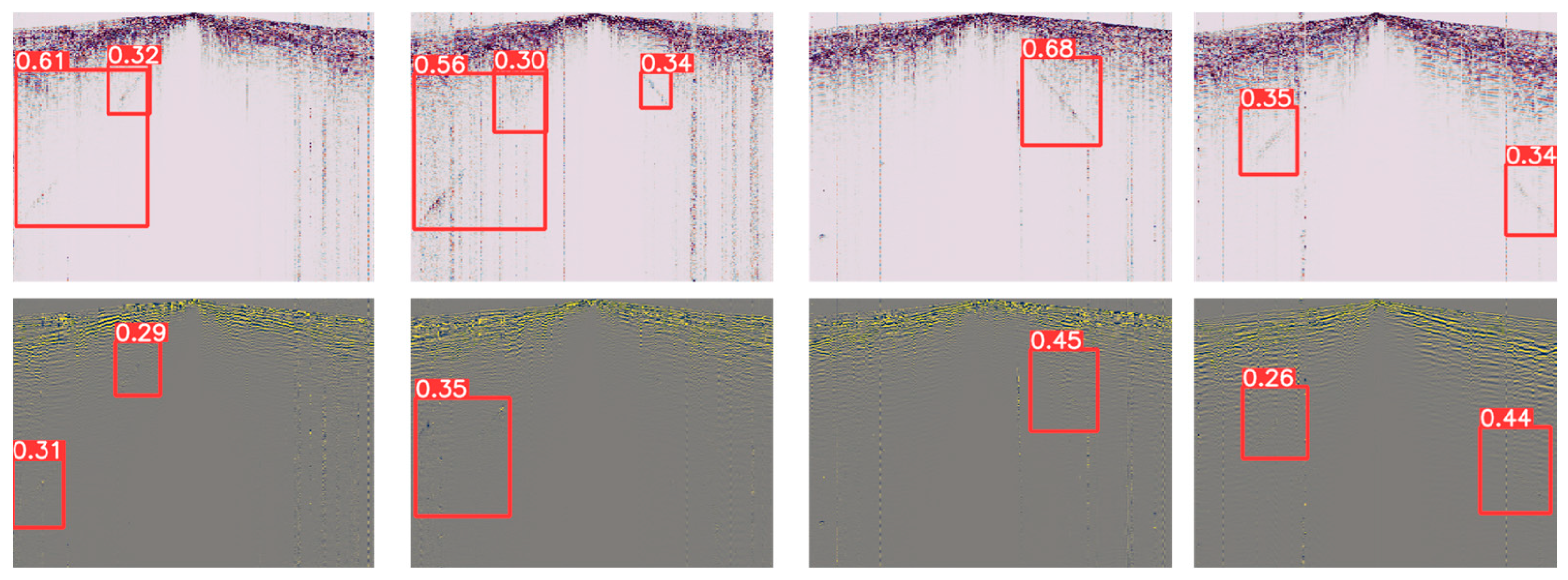
Our model underwent secondary training based on the initial weights of YOLOv5m, which were obtained through pre-training on a large dataset. Specifically, the initial weights of YOLOv5m are typically pre-trained on the COCO (Common Objects in Context) dataset [49]. The COCO dataset is a standard resource that contains hundreds of thousands of annotated images across 80 categories, widely utilized for various tasks in the field of computer vision.
Utilizing these pre-trained weights enables the model to recognize common object features right from the start of secondary training (Figure 4). This capability allows the model to achieve good detection results in a shorter timeframe, thereby reducing overall training time and enhancing final performance.
To facilitate the secondary training and fine-tuning of YOLOv5m for detecting airwave noise, we constructed a dedicated training dataset. The samples were collected from 5000 two-dimensional seismic recordings gathered in Ningqiang County, Shaanxi Province, in August 2023. This area presents complex seismic geological conditions characterized by significant terrain fluctuations and numerous cliffs. The exposed strata range from the Jurassic to the Sinian period, predominantly consisting of layers from the Triassic, Sinian, and Proterozoic. Notably, the dip angles of these strata vary considerably, typically between 45° and 70°. The lithology is primarily limestone, with lower proportions of sandstone and mudstone, leading to overall poor excitation and reception conditions, which results in substantial airwave noise.
In our dataset, we manually marked the locations of airwave noise in each sample, as illustrated by the green boxes in Figure 1. After screening, we identified a total of 580 samples exhibiting clear airwave noise, with 80% allocated for training and 20% for testing. The training and prediction processes were accelerated using a GPU (NVIDIA GeForce RTX 3070 with 128 GB of memory (NVIDIA Corporation, Santa Clara, CA, USA)). The secondary training comprised a total of 100 iterations, taking approximately 1 h to complete. Upon finishing the training, the prediction time for a single two-dimensional seismic recording was under 0.5 s, while the prediction time for three-dimensional seismic recordings was under 2 s.
Due to the slower propagation speed of airwaves compared to seismic waves, the acquisition window often closes before the acoustic waves reach the distant detectors. As a result, airwaves are only observed within a radius R a = v a t around the source, where v a is speed of airwaves propagation and t is travel time. To enhance prediction efficiency, we crop the original seismic images, selecting only a portion of the seismic recordings for analysis. For two-dimensional seismic recordings, we extract data centered around the source with a radius of R a . In the case of three-dimensional seismic recordings, we extract seismic data from a rectangular area defined by R a × 0.7 R a , treating each two-dimensional profile line as an individual sample.
After preparing all the data, we construct profile images from the two-dimensional seismic recordings to serve as input for the model. To ensure consistent input dimensions, the samples undergo pixel interpolation. The 2D seismic data with one channel needs to be first mapped into images with three RGB color channels during training and prediction process (Figure 4). The model then outputs the locations of airwave noise along with their corresponding confidence.
Figure 5 illustrates the evolution curves of loss and precision-recall during the secondary training process of YOLOv5m. As shown in the figure, both the localization loss and confidence loss for the training set decrease rapidly, while the precision and recall steadily increase. This indicates that the model performs well in learning the mapping from two-dimensional seismic images to airwave locations. Specifically, precision refers to the proportion of actual positive samples among those predicted as positive (i.e., indicating the presence of airwave noise) by the model, while recall represents the proportion of correctly predicted positive samples out of all actual positive samples.

5. Results

Figure 6 shows the statistical distribution of the test dataset samples. In Figure 6a, the predicted locations of airwave noise closely align with the actual positions, with the coordinate origin at the top-left corner of the predicted image. This creates an “inverted V” pattern in the distribution of airwave noise. In Figure 6b, the width of the predicted bounding boxes varies linearly with height, as the boxes for airwave noise are not elongated (see Figure 1). Figure 6c illustrates the precision and recall curves as a function of the confidence threshold. Regions with confidence above the threshold are classified as containing airwave noise. A lower confidence threshold generally yields higher recall and lower precision, meaning the model may produce more false positives but is less likely to miss any detection. On the other hand, a higher confidence threshold results in lower recall but higher precision, reducing false positives while increasing the chance of missed detections.
Figure 7 presents several prediction results from the test dataset. Overall, the model effectively identifies prominent airwave noise, with higher-confidence bounding boxes indicating more pronounced interference. The detection of interference locations is also highly accurate. These results confirm the robustness and effectiveness of the YOLOv5 model.

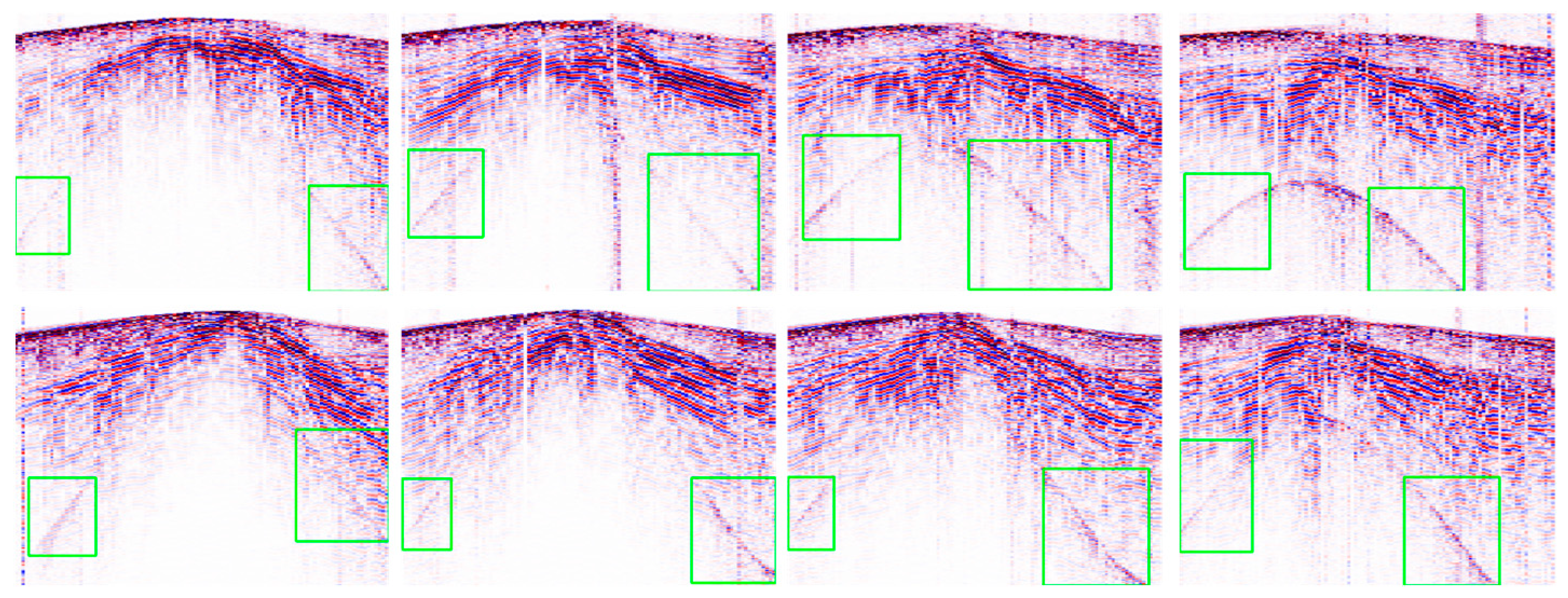
6. Field Data Validation

In practical applications, we usually focus on whether airwave noise is present, rather than pinpointing the airwave region. Moreover, we classify interference as significant only when it is detected on both sides of the seismic source. Interference detected on just one side is not considered significant, as it may result from other sources and may not be strong enough to qualify as substantial interference. To determine the presence of airwave noise, we follow these steps: (1) Extract seismic images from within the acoustic range, based on 2D or 3D seismic records, and use these as input for YOLOv5m; (2) Check the YOLOv5m predictions to see if two predicted targets are detected. If no targets are detected in any input image, airwave noise is considered absent. If targets are detected, proceed to the next step; (3) Assess whether both predicted bounding boxes have confidence scores greater than 0.35 and are spatially separated. For 3D seismic profiles, if at least one image (one line data) contains a pair of boxes meeting these criteria, airwave noise is confirmed; otherwise, it is deemed absent.
To further assess the model’s effectiveness, we tested it using 456 shots of 2D seismic data from the same region, which were excluded from both the training and test datasets. As shown in Table 2, the model achieved an overall accuracy of 96.4% on this dataset, indicating that it can reliably detect the presence or absence of airwave noise in most cases (see Table 2). Notably, in the instances where airwave was present, the model’s recall was significantly higher than its precision, suggesting a tendency towards false positives rather than missed detections. The high values of the Dice Index and Jaccard Index suggest that the model has performed very well in detecting airwave cases. The formulas for different evaluation metrics used are shown as follows:
P r e c i s i o n = T P T P + F P
R e c a l l = T P T P + F N
T P R = T P T P + F N
F P R = F P F P + T N
D i c e = 2 × T P 2 × T P + F P + F N
J a c c a r d = T P T P + F P + F N
where TP = True Positives (correctly predicted positive cases), and FN = False Negatives (actual positives that were incorrectly predicted as negatives); FP = False Positives (actual negatives that were incorrectly predicted as positives); TN = True Negatives (correctly predicted negative cases). TPR measures how well the model can identify positive instances. A higher TPR means fewer false negatives, indicating better performance in detecting positive cases. FPR measures the proportion of actual negative instances that are incorrectly identified as positive by the model. The Dice Index is a measure of overlap between two sets (predicted and actual), commonly used in binary classification tasks, especially in medical imaging and object detection. The Jaccard Index is another measure of similarity between two sets, commonly used to compare the overlap of predicted and actual positive instances.
The model’s recall rate was higher than its performance on the YOLO test dataset (Figure 5), because we defined interference as present if at least one 2D seismic record from a shot satisfied the interference condition, thereby minimizing missed detections. The model’s precision on airwave was slightly lower compared to the YOLO test dataset, because the airwave noises are weak, which was not represented in the training data. In practical applications, such weak interference is usually negligible, but during prediction, it can result in low-confidence scores. When these scores exceed the threshold, they are classified as airwave noise (Figure 8).
To assess the model’s transferability, we applied the model, initially trained on 2D data, to 55 shots of 3D seismic exploration data collected from the Xiushui Town area in Sichuan, China. The predictions are partially illustrated in Figure 9. For the points close to the seismic source, the airwave noise appears as symmetrical diagonal lines, closely resembling predictions from the 2D records. In contrast, for survey lines farther from the source, the interference takes on an arc-shaped pattern, which differs from the 2D seismic recordings. Nonetheless, the model perform well, accurately predicting the airwave on both sides of the arc.
As shown in Table 3, the overall prediction accuracy in this region reached 94%, surpassing the results obtained in the Qiangning area. The values of the Dice Index and Jaccard Index are higher than that in 2D case, suggesting a good performance in detecting 3D airwave cases. In addition, the missed detections were primarily attributed to the airwave being too weak to exceed the confidence threshold of 0.35. These findings confirm that the proposed model possesses strong predictive accuracy and robust generalization capabilities.
Furthermore, the YOLOv5m model demonstrated its ability to identify unilateral acoustic waves (Figure 10). When the shot point is positioned near a mountain, the terrain can obstruct and reflect the propagation path of the acoustic waves. This results in the waves being reflected and absorbed on the mountain side, leading to a predominance of wave propagation toward the flat side, which creates the unilateral airwave wave phenomenon. Since this type of interference is mainly caused by the terrain, it can generally be disregarded in practical evaluations unless the interference energy is exceptionally high.

7. Discussion

We compared the training and testing results of all models within the YOLOv5 family: YOLOv5l, YOLOv5m, YOLOv5s, and YOLOv5n. These models exhibit differences in parameter quantities, network scales, and computational costs, with YOLOv5m achieving a better balance between computational precision, efficiency, and storage space (Table 4).
The YOLO model is a method based on computer vision, so 2D seismic data needs to be first mapped into images during the training and prediction process. OpenCV provides a variety of predefined color mappings that can map pixel intensity values in grayscale images to color values, commonly used in scientific data visualization or image processing [50]. Different mappings exhibit varying performance in identifying airwave anomalies. In this study, through testing multiple mappings, we selected TWILIGHT as the primary color mapping for training and prediction samples. Table 5 and Figure 11 show the prediction performance for different mappings, where TWILIGHT demonstrates significantly higher accuracy compared to CIVIDIS.

8. Conclusions

In recent years, significant advancements in neural network technology, driven by rapid increases in computational power, have led to its widespread application across various fields, including Earth sciences [20,23,51,52,53]. While manual identification of airwave noise can be somewhat intuitive, processing vast amounts of three-dimensional seismic data through manual operations is not only time-consuming but also introduces subjective judgment. This paper effectively addresses these challenges through the application of YOLOv5.
We present a comprehensive workflow for identifying airwave noise in seismic data based on YOLOv5m, encompassing model construction, loss function establishment, dataset creation, model training, and prediction. Training results indicate that the model achieves an accuracy and recall of approximately 85% on the test dataset, successfully predicting airwave noise locations and confidence levels.
To further validate the model’s effectiveness, we applied the YOLOv5m model, trained on two-dimensional data, to seismic records from the Ningqiang area of Shaanxi and three-dimensional seismic records from the Xiushui area of Sichuan. The overall prediction accuracy in both regions exceeded 90%, with accuracy and recall rates for airwave noise reaching over 83% and 90%, respectively. Notably, the evaluation speed for single-shot three-dimensional seismic data (over 8000 traces) was less than 2 s, demonstrating the model’s excellent transferability, generalization ability, and efficiency, making it suitable for detecting airwave noise in raw seismic data across diverse regions. Additionally, our algorithm can differentiate between unilateral and bilateral airwave noise, facilitating a comprehensive assessment of seismic data quality.
This study represents the first automated, real-time detection of airwave noise, significantly enhancing operational efficiency. It also enables timely noise reduction measures, improving data quality and, consequently, increasing the reliability and accuracy of seismic data processing. This method can be extended to the recognition of various seismic signals or noise signals, which will be part of our future work.

Author Contributions

Conceptualization, Z.L., Z.Z. and L.G.; methodology, Z.L., L.G., F.S. and R.T.; validation, Z.Z., F.S. and X.H.; writing—original draft preparation, Z.L. and L.G.; writing—review and editing, L.G., X.H. and R.T.; visualization, X.H. and G.C.; supervision, R.T.; funding acquisition, Z.Z. and X.H. All authors have read and agreed to the published version of the manuscript.

Funding

This work is supported by the Sinopec Data Intelligent Collection Research Project and Huzhou Public Welfare Research Project (2023GZ17).

Institutional Review Board Statement

Not applicable for studies not involving humans or animals.

Informed Consent Statement

Not applicable.

Data Availability Statement

Data and codes cannot be disclosed due to commercial confidentiality.

Conflicts of Interest

Authors Zhenghong Liang, Zhifeng Zhang and Xiuju Huang were employed by the Sinopec Petroleum Engineering Geophysics Co., Ltd. The remaining authors declare that the research was conducted in the absence of any commercial or financial relationships that could be construed as a potential conflict of interest.

References

  1. Cai, X. Adaptive detection and suppression method for sub-frequency division of acoustic waves and strong energy interference. Oil Geophys. Explor. 1999, 34, 373–380. [Google Scholar]
  2. Mondol, N.H. Seismic exploration. In Petroleum Geoscience: From Sedimentary Environments to Rock Physics; Springer Science & Business Media: Berlin/Heidelberg, Germany, 2015; pp. 427–454. [Google Scholar]
  3. Karastathis, V.; Louis, I.F. The airwave in hammer reflection seismic data. Bol. Geofis. Teor. Appl 1997, 39, 13–23. [Google Scholar]
  4. Meunier, J. Seismic Acquisition from Yesterday to Tomorrow; Society of Exploration Geophysicists: Tulsa, OK, USA, 2011. [Google Scholar]
  5. Talagapu, K.K. 2D and 3D Land Seismic Data Acquisition and Seismic Data Processing; Department of Geophysics, College of Science and Technology, Andhra University: Visakhapatnam, India, 2005. [Google Scholar]
  6. Wang, Y.; Zhang, G.; Chen, T.; Liu, Y.; Shen, B.; Liang, J.; Hu, G. Data and model dual-driven seismic deconvolution via error-constrained joint sparse representation. Geophysics 2023, 88, 1–112. [Google Scholar] [CrossRef]
  7. Cui, X. Seismic acquisition quality monitoring under complex geological conditions. Oil Geophys. Explor. 2003, 1, 11–16. [Google Scholar]
  8. Luo, W. Research and Application of Seismic Data Acquisition Quality Control Technology. Ph.D. Thesis, Southwest Petroleum University, Chengdu, China, 2016. [Google Scholar]
  9. Tian, C.; Cheng, Y. Research and application of field seismic data acquisition quality monitoring technology. Complex Oil Gas Reserv. 2011, 4, 25–27. [Google Scholar]
  10. Zhao, Z.; Ding, J. On-site quality monitoring technology for seismic data acquisition. Inn. Mong. Petrochem. 2009, 35, 98–99. [Google Scholar]
  11. Mousavi, S.M.; Beroza, G.C. Deep-learning seismology. Science 2022, 377, eabm4470. [Google Scholar] [CrossRef]
  12. Wang, Y.; Qiu, Q.; Lan, Z.; Chen, K.; Zhou, J.; Gao, P.; Zhang, W. Identifying microseismic events using a dual-channel CNN with wavelet packets decomposition coefficients. Comput. Geosci. 2022, 166, 105164. [Google Scholar] [CrossRef]
  13. Gan, L.; Wu, Q.; Huang, Q.; Tang, R. Quality classification and inversion of receiver functions using convolutional neural network. Geophys. J. Int. 2023, 232, 1833–1848. [Google Scholar] [CrossRef]
  14. Zhang, X.; Mao, L.; Yang, Y.; Zhou, Z. Study on the noise reduction method for semiaerial transient electromagnetic data based on LSTM. Comput. Tech. Geophys. Geochem. Explor. 2024, 46, 423–433. [Google Scholar]
  15. Li, Q.; Wang, X.; Zhang, Y.; Wen, X.; Chen, Y.; Wang, C.; Liao, W. Fault recognition method and application based on 3D U-Net++convolution neural network. Comput. Tech. Geophys. Geochem. Explor. 2024, 46, 284–291. [Google Scholar]
  16. Feng, Q.; Li, Y. Denoising deep learning network based on singular spectrum analysis—DAS seismic data denoising with multichannel SVDDCNN. IEEE Trans. Geosci. Remote Sens. 2021, 60, 1–11. [Google Scholar] [CrossRef]
  17. Li, W.; Liu, H.; Wang, J. A Deep learning method for denoising based on a fast and flexible convolutional neural network. IEEE Trans. Geosci. Remote Sens. 2021, 60, 5902813. [Google Scholar] [CrossRef]
  18. Tibi, R.; Young, C.J.; Porritt, R.W. Comparative Study of the Performance of Seismic Waveform Denoising Methods Using Local and Near-Regional Data. Bull. Seism. Soc. Am. 2023, 113, 548–561. [Google Scholar] [CrossRef]
  19. Li, S.; Liu, B.; Ren, Y.; Chen, Y.; Yang, S.; Wang, Y.; Jiang, P. Deep-learning inversion of seismic data. arXiv 2019, arXiv:1901.07733. [Google Scholar] [CrossRef]
  20. Zheng, Y.; Zhang, Q.; Yusifov, A.; Shi, Y. Applications of supervised deep learning for seismic interpretation and inversion. Lead. Edge 2019, 38, 526–533. [Google Scholar] [CrossRef]
  21. Gao, Y.; Li, H.; Li, G.; Wei, P.; Zhang, H. Deep learning for high-resolution multichannel seismic impedance inversion. Geophysics 2024, 89, WA323–WA335. [Google Scholar] [CrossRef]
  22. Tang, R.; Li, F.; Shen, F.; Gan, L.; Shi, Y. Fast forecasting of water-filled bodies position using transient electromagnetic method based on deep learning. IEEE Trans. Geosci. Remote Sens. 2024, 62, 4502013. [Google Scholar] [CrossRef]
  23. Tang, R.; Gan, L.; Li, F.; Shen, F. A Fast Three-dimensional Imaging Scheme of Airborne Time Domain Electromagnetic Data using Deep Learning. TechRxiv 2024. [Google Scholar] [CrossRef]
  24. Zhao, Z.Q.; Zheng, P.; Xu, S.T.; Wu, X. Object detection with deep learning: A review. IEEE Trans. Neural Netw. Learn. Syst. 2019, 30, 3212–3232. [Google Scholar] [CrossRef]
  25. Shao, F.; Chen, L.; Shao, J.; Ji, W.; Xiao, S.; Ye, L.; Zhuang, Y.; Xiao, J. Deep learning for weakly-supervised object detection and localization: A survey. Neurocomputing 2022, 496, 192–207. [Google Scholar] [CrossRef]
  26. Kellenberger, B.; Marcos, D.; Tuia, D. Detecting mammals in UAV images: Best practices to address a substantially imbalanced dataset with deep learning. Remote Sens. Environ. 2018, 216, 139–153. [Google Scholar] [CrossRef]
  27. Kellenberger, B.; Volpi, M.; Tuia, D. Fast animal detection in UAV images using convolutional neural networks. In Proceedings of the 2017 IEEE International Geoscience and Remote Sensing Symposium, IGARSS 2017, Fort Worth, TX, USA, 23–28 July 2017; IEEE: New York, NY, USA, 2017; pp. 866–869. [Google Scholar]
  28. Audebert, N.; Boulch, A.; Le Saux, B.; Lefèvre, S. Distance transform regression for spatially-aware deep semantic segmentation. Comput. Vis. Image Underst. 2019, 189, 102809. [Google Scholar] [CrossRef]
  29. Redmon, J.; Farhadi, A. YOLO9000: Better, faster, stronger. In Proceedings of the IEEE Conference on Computer Vision and Pattern Recognition, Honolulu, HI, USA, 21–26 July 2017; pp. 7263–7271. [Google Scholar]
  30. Redmon, J.; Farhadi, A. Yolov3: An incremental improvement. arXiv 2018, arXiv:1804.02767. [Google Scholar]
  31. Redmon, J.; Divvala, S.; Girshick, R.; Farhadi, A. You only look once: Unified, real-time object detection. In Proceedings of the IEEE Conference on Computer Vision and Pattern Recognition, Las Vegas, NV, USA, 27–30 June 2016; pp. 779–788. [Google Scholar]
  32. Bochkovskiy, A. YOLOv4: Optimal Speed and Accuracy of Object Detection. arXiv 2020, arXiv:2004.10934. [Google Scholar]
  33. Jocher. YOLOv5 by Ultralytics. 2020. Available online: https://github.com/ultralytics/yolov5 (accessed on 1 December 2024).
  34. Wang, S.; Pan, H.; Weifeng, G.; Bian, C.; Zhang, X.; Dong, B. YOLO-DCANet: Seismic velocity spectrum picking method based on deformable convolution and attention mechanism. In Proceedings of the Fifth International Conference on Geology, Mapping, and Remote Sensing (ICGMRS 2024), Wuhan, China, 12–14 April 2024; SPIE: Bellingham, WA, USA, 2024; Volume 13223, pp. 559–564. [Google Scholar]
  35. Pang, D.; Liu, G.; He, J.; Li, W.; Fu, R. Automatic remote sensing identification of co-seismic landslides using deep learning methods. Forests 2022, 13, 1213. [Google Scholar] [CrossRef]
  36. Zhu, X.; Shragge, J. Toward real-time microseismic event detection using the YOLOv3 algorithm. Earth arXiv 2022. preprint. [Google Scholar]
  37. Wang, D.; Zhang, Y.; Zhang, R.; Nie, G.; Wang, W. Detection and assessment of post-earthquake functional building ceiling damage based on improved YOLOv8. J. Build. Eng. 2024, 98, 111315. [Google Scholar] [CrossRef]
  38. Lee, D.; Choi, S.; Lee, J.; Chung, W. Efficient seismic numerical modeling technique using the yolov2-based expanding domain method. J. Seism. Explor. 2022, 31, 425–449. [Google Scholar]
  39. Li, J.; Li, K.; Tang, S. Automatic arrival-time picking of P- and S-waves of microseismic events based on object detection and CNN. Soil Dyn. Earthq. Eng. 2023, 164, 107560. [Google Scholar] [CrossRef]
  40. Park, S.; Kim, J.; Jeon, K.; Kim, J.; Park, S. Improvement of gpr-based rebar diameter estimation using yolo-v3. Remote Sens. 2021, 13, 2011. [Google Scholar] [CrossRef]
  41. Ilmak, D.; Iban, M.C.; Şeker, D.Z. A Geospatial Dataframe of Collapsed Buildings in Antakya City after the 2023 Kahramanmaraş Earthquakes Using Object Detection Based on Yolo and VHR Satellite Images. In Proceedings of the IGARSS 2024—2024 IEEE International Geoscience and Remote Sensing Symposium, Athens, Greece, 7–12 July 2024; pp. 3915–3919. [Google Scholar]
  42. Li, J.; Meng, J.B.; Li, P. Detecting the Bull’s-Eye Effect in Seismic Inversion Low-Frequency Models Using the Optimized YOLOv7 Model. Appl. Geophys. 2024, 1–11. [Google Scholar] [CrossRef]
  43. Kustu, T.; Taskin, A. Deep learning and stereo vision based detection of post-earthquake fire geolocation for smart cities within the scope of disaster management: İstanbul case. Int. J. Disaster Risk Reduct. 2023, 96, 103906. [Google Scholar] [CrossRef]
  44. Zhang, Y.; Guo, Z.; Wu, J.; Tian, Y.; Tang, H.; Guo, X. Real-time vehicle detection based on improved YOLO v5. Sustainability 2022, 14, 12274. [Google Scholar] [CrossRef]
  45. Khanam, R.; Hussain, M. What is YOLOv5: A deep look into the internal features of the popular object detector. arXiv 2024, arXiv:2407.20892. [Google Scholar]
  46. Chen, F.; Zhang, L.; Kang, S.; Chen, L.; Dong, H.; Li, D.; Wu, X. Soft-NMS-enabled YOLOv5 with SIOU for small water surface floater detection in UAV-captured images. Sustainability 2023, 15, 10751. [Google Scholar] [CrossRef]
  47. Miao, F.; Yao, L.; Zhao, X. Adaptive margin aware complement-cross entropy loss for improving class imbalance in multi-view sleep staging based on eeg signals. IEEE Trans. Neural Syst. Rehabil. Eng. 2022, 30, 2927–2938. [Google Scholar] [CrossRef]
  48. Ding, J.; Cao, H.; Ding, X.; An, C. High accuracy real-time insulator string defect detection method based on improved YOLOv5. Front. Energy Res. 2022, 10, 928164. [Google Scholar] [CrossRef]
  49. Liu, W.; Quijano, K.; Crawford, M.M. YOLOv5-Tassel: Detecting tassels in RGB UAV imagery with improved YOLOv5 based on transfer learning. IEEE J. Sel. Top. Appl. Earth Obs. Remote Sens. 2022, 15, 8085–8094. [Google Scholar] [CrossRef]
  50. Sharma, A.; Pathak, J.; Prakash, M.; Singh, J.N. Object detection using OpenCV and python. In Proceedings of the 2021 3rd international Conference on Advances in Computing, Communication Control and Networking (ICAC3N), Greater Noida, India, 17–18 December 2021; IEEE: New York, NY, USA, 2021; pp. 501–505. [Google Scholar]
  51. Hegde, J.; Rokseth, B. Applications of machine learning methods for engineering risk assessment—A review. Saf. Sci. 2020, 122, 104492. [Google Scholar] [CrossRef]
  52. Shi, Y.; Liao, J.; Gan, L.; Tang, R. Lithofacies Prediction from Well Log Data Based on Deep Learning: A Case Study from Southern Sichuan, China. Appl. Sci. 2024, 14, 8195. [Google Scholar] [CrossRef]
  53. Gan, L.; Tang, R.; Li, F.; Shen, F. A Deep learning estimation for probing Depth of Transient Electromagnetic Observation. Appl. Sci. 2024, 14, 7123. [Google Scholar] [CrossRef]
Figure 1. Typical characteristics of airwave noise (indicated in green). (a) No airwave noise; (b) Weak airwave noise; (c,d) represent airwave noise in three-dimensional exploration, where (c) is closer to the seismic source than (d); (e,f) depict typical airwave noise in two-dimensional seismic exploration.
Applsci 14 11636 g001
Figure 2. The YOLOv5m network architecture (modified from Zhang, 2022 [44]). Conv refers to two-dimensional convolution operations, while BN (Batch Normalization) accelerates network convergence during training and reduces sensitivity to parameter initialization. Concat denotes the concatenation operation used to merge features from different sources. SiLU is the activation function, defined as S i L U x = x 1 + e x , which is a smooth, nonlinear activation function. This means that it does not introduce discontinuity at zero like ReLU (Rectified Linear Unit), thereby avoiding gradient instability issues. MaxPool refers to the max pooling layer used for downsampling, which reduces the size of the feature map by selecting the maximum value within local regions of the feature map, while preserving the most significant features.
Applsci 14 11636 g002
Figure 3. The diagram illustrates the grid division (black grid lines), marked boxes or label (yellow bounding boxes), prior anchor boxes (red bounding boxes), and the non-maximum suppression process. Since only one class is predicted, each predicted unit greater than the IoU threshold (indicated in purple) corresponds to three anchor boxes, which are merged into one by the non-maximum suppression algorithm. (Modified form https://cloud.tencent.com/developer/article/1118040 (accessed on 1 January 2020)).
Applsci 14 11636 g003
Figure 4. YOLOv5 training and prediction workflow for airwave detection in seismic profiles. The pentagram represents the source location.
Applsci 14 11636 g004
Figure 5. The evolution curves of loss and precision-recall during the secondary training of YOLOv5m.
Applsci 14 11636 g005
Figure 6. Statistical distribution of samples in the test dataset: (a) A distribution map of predicted locations of airwave noise, where x and y represent the two spatial dimensions of the image, with the top-left corner of the image set as the coordinate origin. (b) Statistical distribution of widths and heights of predicted airwave noise boxes. (c) The relationship between recall and accuracy at different confidence levels.
Applsci 14 11636 g006
Figure 7. Randomly selected predictions from the test dataset, where the red boxes indicate airwave noise detected by YOLOv5m, and the numbers in the top-left corner represent the confidence levels.
Applsci 14 11636 g007
Figure 8. Instances labeled as no interference but predicted as interference; the boxes represent the prediction results, and the numbers indicate the confidence levels.
Applsci 14 11636 g008
Figure 9. Randomly selected airwave noise prediction results from the Xiushui three-dimensional seismic data. The green boxes indicate YOLOv5m predictions of airwave noise, with the first and second rows representing seismic records corresponding to different seismic sources.
Applsci 14 11636 g009
Figure 10. The 3D seismic records in the Xiushui area exhibit unilateral airwave noise, primarily caused by the terrain.
Applsci 14 11636 g010
Figure 11. Airwave predictions of different colormap in test dataset, and the numbers in the top-left corner represent the confidence levels. Up: TWILIGHT. Down: CIVIDIS.
Applsci 14 11636 g011
Table 1. Applications of the YOLO object detection algorithm in seismology.
Application DescriptionReference
Seismic velocity spectrum pickingWang et al., 2024 [37]
Real-time co-seismic landslide detectionPang et al., 2022 [35]
Detection of co-seismic collapsed buildingsWang et al., 2024 [37]
Ilmak and Iban, 2024 [41]
Microseismic event detectionZhu and Shragge, 2022 [36]
Local velocity anomalies detection from Seismic inversion modelsLi and Meng, 2024 [42]
Seismic numerical modelingLee et al., 2022 [38]
Arrival-time picking of P- and S-waves of microseismic eventsLi et al., 2023 [39]
Post-earthquake fire detectionKustu and Taskin, 2023 [43]
Seismic noise detection (this work)
Table 2. Predictions of airwave noise in the 456-shot two-dimensional seismic records from Ningqiang County (accuracy and recall statistics).
CategoryPrecisionRecallF1-ScoreSupportTPRFPRDice IndexJaccard Index
0 (No airwave)1.00.980.994100.95650.02200.88890.8
1 (airwave)0.830.960.8946
Table 3. Predictions of airwave noise in the 54-shot 3D seismic records from Xiushui County.
CategoryPrecisionRecallF1-ScoreSupportTPRFPRDice IndexJaccard Index
0 (No airwave)0.941.00.97311.00.060.9540.913
1 (airwave)1.00.910.9523
Table 4. Comparison of YOLOv5 family training.
Train Time (h)PrecisionRecallmAP@0.5mAP50:95Inference (ms)Parameter (MB)FLOPs@640 (B)
yolov5l0.880.99710.9950.9810.146.5109.1
yolov5m0.5540.9710.9950.9458.221.249
yolov5s0.3180.9870.9510.9920.8476.47.216.5
yolov5n0.240.9750.940.9920.7726.31.94.5
Note: mAP@0.5 (Mean Average Precision at IoU = 0.5 thresholds); mAP@0.5:0.95 (Mean Average Precision at IoU = 0.5:0.95 thresholds); FLOPs@640 refers to the number of floating-point operations.
Table 5. Comparison of YOLOv5 test result of Twilight and Cividis colormap.
PRmAP50mAP50:95
Twilight0.9710.9950.945
Cividis0.8250.850.8260.805
Disclaimer/Publisher’s Note: The statements, opinions and data contained in all publications are solely those of the individual author(s) and contributor(s) and not of MDPI and/or the editor(s). MDPI and/or the editor(s) disclaim responsibility for any injury to people or property resulting from any ideas, methods, instructions or products referred to in the content.

