Measuring Collision Risk in Mixed Traffic Flow Under the Car-Following and Lane-Changing Behavior

Abstract

This study proposes a risk measurement approach to assess collision risks in mixed traffic flow, focusing on the integrated behavior of car-following and lane-changing. A new surrogate safety measure (SSM), denoted as $R_{\mathrm{total}}$, is developed to provide a comprehensive risk assessment. Numerical analysis is used to determine the weights of parameters within $R_{\mathrm{total}}$, and its validity is substantiated using an empirical dataset, with a risk threshold of 0.49 established when the time to collision (TTC) is set to 2 s. The study incorporates scenarios of connected and automated vehicle (CAV) degradation and evaluates the influence of penetration rates, perception–reaction time (PRT), and lane-changing modes on risk levels. Simulation results reveal that a CAV penetration rate between 0.4 and 0.6 represents a critical range where collision risks significantly increase, reflecting safety dynamics under CAV degradation. Furthermore, in scenarios involving lane-changing, the degradation of the following vehicle in the target lane poses the highest risk. At lower PRTs, the penetration rate exerts a more significant influence on collision risks. $R_{\mathrm{total}}$ has been validated across various scenarios, showing strong applicability and more sensitive trends than other SSMs, making it well-suited for assessing long-term comprehensive traffic flow risks. These findings offer practical guidance for traffic management to establish real-time risk prediction and warning systems for identifying high-risk car-following and lane-changing behaviors. Future research can explore the applicability of the proposed risk index in more complex traffic scenarios and its effectiveness across different levels of vehicle automation and connectivity.

1. Introduction

In the rapidly advancing era of intelligent transportation, connected and autonomous vehicles (CAVs) have emerged as a crucial solution for mitigating traffic congestion [1] and enhancing road safety [2]. The introduction of this new mixed traffic paradigm has created a complex, dynamic, and boundaryless traffic flow, highlighting the growing importance of highway safety management. As a result, the assessment of highway traffic operational risks and the assurance of safety and efficiency have become critical areas of research, particularly within the transportation field.

Traditional traffic safety research, which primarily relies on historical crash data to establish connections between crash frequencies or severities and contributing factors, faces several challenges: (i) Traffic accidents, accounting for less than 0.01% of all traffic incidents on highways, exhibit characteristics of low probability, high randomness, and unpredictability, making them difficult to directly observe in real-world scenarios; (ii) historical crash data cannot be utilized for real-time or ex-ante analyses [3]. A promising alternative to overcome these limitations involves the use of near-crash or traffic conflict data [4], which occur far more frequently than crashes and provide valuable insights for estimating the safety performance of entities on the road network [5]. Moreover, numerous studies have established statistically significant associations between traffic conflicts and observed crashes [6,7,8].

Since the late 20th century, Surrogate Safety Measures (SSMs) have garnered significant attention and recognition in the field of road traffic safety analysis. With ongoing advancements in traffic collision analysis technologies, new SSMs that go beyond conventional metrics of time, distance, and speed reduction have also emerged. SSMs have contributed substantially to improving transportation safety across diverse domains, including infrastructure assessment, user behavior analysis, and emerging technology evaluation [9], ultimately supporting policy and strategy development [8].

Recently, SSMs have gained particular prominence in conflict-based analyses, owing to their capability to identify the temporal or spatial proximity of road users, which facilitates the detection, evaluation, and severity assessment of conflicts or near-misses [10]. In modern research, SSMs are crucial for evaluating CAV safety during their developmental phases. Given the scarcity of historical and generalizable safety data on CAVs, microsimulation techniques that extract vehicle trajectories and identify traffic conflicts through SSMs have proven effective in addressing data limitations while ensuring robust safety assessment methodologies for emerging autonomous technologies [9]. However, most simulation environments for safety analysis, which are often restricted to single-lane scenarios, fail to consider the impact of vehicle information interaction within a networked communication context or the effects of lane-changing behavior on safety. Consequently, the SSMs proposed for mixed traffic flows, including CAVs, are predominantly applicable to car-following risks without adequately considering lateral risks.

Research on CAVs has gained significant attention due to their potential to improve safety and traffic operations. However, the technology is not yet mature enough for large-scale deployment. Despite real-world trials and advancements, autonomous vehicles (AVs) are still far from widespread adoption, particularly in safety evaluation [11]. A transition phase involving mixed traffic, where human-driven vehicles (HDVs), AVs, and CAVs coexist, is expected to persist for a long time [12]. Thus, CAV studies largely rely on microscopic traffic simulations, and SSMs have been widely adopted to quantify CAV safety benefits based on these simulations [4].

When a CAV follows an HDV, it cannot achieve cooperative driving due to communication limitations, resulting in the degradation of Cooperative Adaptive Cruise Control (CACC) to Adaptive Cruise Control (ACC) mode. This degradation phenomenon has been extensively studied. For instance, Tu [13] evaluated the safety impact of CACC degradation on collision risk using the TIT index, finding that sudden deceleration of the leading vehicle significantly increases collision risk. Qin [14] analyzed the stability and safety of mixed traffic flow with varying CV penetration rates when connected vehicles (CVs) degrade to regular vehicles. Yao [15] studied CACC vehicles’ degradation into ACC mode due to communication failures, noting that this significantly raises the safety risks in mixed traffic.

These studies considered the functional degradation of CAVs but did not consider the perception–reaction time (PRT) of CAVs. The PRT of intelligent vehicle systems is crucial for evaluating performance, encompassing perception time, decision time, and control time. Compared to HDVs, CAVs have a shorter PRT. Some researchers have conceptually considered time lags in PRT. Li [16] included the perception–reaction time factor and the safe time headway factor in the ACC model. Peng [17] designed a new heterogeneous lattice hydrodynamic model, incorporating CAVs and HDVs, to explore the feedback control effect of delayed differences for different vehicle types. In summary, few studies have considered both the degradation of CAVs and their PRT.

Based on the previous discussion, we conducted a search in Scopus to review studies published since 2017. The search used the keywords “mixed traffic flow”, “collision risk”, “car-following behavior”, “lane-changing behavior”, “CAV degradation”, and “perception-reaction time”, as well as their combinations. While several studies address individual factors or partial combinations, no research comprehensively considers all of them.

Therefore, the primary objective of this study is to develop a new comprehensive SSM designed to quantify collision risks in mixed traffic flow. This new SSM considers the combined effects of longitudinal and lateral vehicle interactions. By comparing it with other typical SSMs, the proposed index evaluates the impacts of CAV degradation and PRT, highlighting the differences between these metrics. Through the design, validation, and application of this novel measure, we aim to address the existing research gap regarding the combined effects of CAV degradation and PRT, thereby providing a more scientific tool for the quantitative assessment of safety in mixed traffic flow.

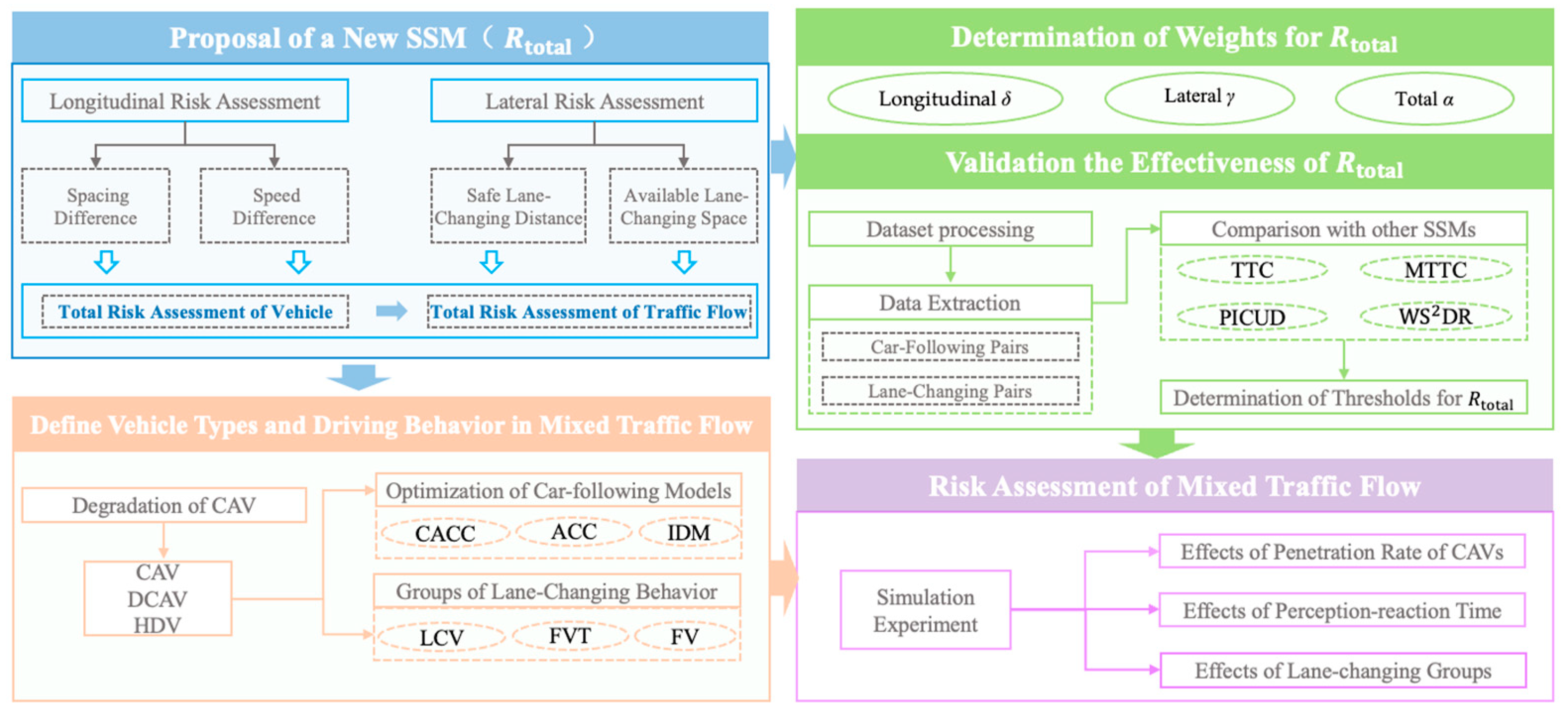
The flowchart of the proposed methodology is shown in Figure 1. The main contributions of this study are summarized as follows:

(1)

We introduce a new SSM that incorporates both longitudinal and lateral factors. This metric, denoted as $R_{\mathrm{t}\mathrm{o}\mathrm{t}\mathrm{a}\mathrm{l}}$, is utilized to assess the risk level of mixed traffic flow;

(2)

The weight of each parameter within $R_{\mathrm{t}\mathrm{o}\mathrm{t}\mathrm{a}\mathrm{l}}$ is ascertained through numerical analysis. The validity of $R_{\mathrm{t}\mathrm{o}\mathrm{t}\mathrm{a}\mathrm{l}}$ is substantiated using an empirical dataset, and the risk threshold is derived;

(3)

$R_{\mathrm{t}\mathrm{o}\mathrm{t}\mathrm{a}\mathrm{l}}$ is used to assess the impact of penetration rate, PRT, and lane-changing combinations on mixed traffic flow safety, contributing to a deeper understanding of safety in mixed-traffic environments

The structure of this paper is as follows. Section 2 provides an overview and analysis of widely used SSMs. Section 3 introduces a new SSM (R_total), detailing the determination of weights and thresholds and validation of its effectiveness. Section 4 optimizes the longitudinal car-following model considering CAV degradation and determines combinations of typical lateral lane-changing behaviors. It further presents the simulation experiments for risk assessment and the analysis of the results. Lastly, Section 5 summarizes the key findings of our study and outlines future research directions in this field.

2. Existing Surrogate Safety Measures (SSMs)

2.1. Time-Based SSMs

Time-based SSMs have been widely used in safety research, the most prominent example of which is Time to Collision (TTC). TTC was proposed by Hayward [18] and predicts the time remaining until a collision occurs by analyzing future vehicle trajectories. It assumes that both vehicles maintain their current velocities. TTC is especially useful for analyzing potential rear-end collision risks. The calculation of TTC is given by Equation (1).

$$\mathrm{T}\mathrm{T}\mathrm{C}={\displaystyle \frac{D}{\Delta v}}$$

(1)

where

$D=x_l-x_f-l$ is the distance between the leading vehicle and the following vehicle, calculated as the difference between the positions of the leading vehicle $x_l$ and the following vehicle $x_f$, minus the length of the leading vehicle $l$.

$\Delta v=v_f-v_l$ is the relative speed between the following vehicle and the leading vehicle, where $v_f$ is the speed of the following vehicle and $v_l$ is the speed of the leading vehicle.

It is important to note that TTC is only applicable when the relative speed $\Delta v$ is non-zero. If $\Delta v=0$, TTC cannot be defined as the two vehicles are moving at the same speed, and a collision will not occur under these circumstances.

Modified Time to Collision (MTTC) was proposed to address the limitations of TTC [19], particularly its inability to account for the effects of acceleration and deceleration during potential collision scenarios. Unlike TTC, MTTC takes into consideration the acceleration differences between vehicles, making it more suitable for analyzing complex driving conditions such as lane changes, merging, and other dynamic traffic situations.

The calculation of MTTC is based on the Equations (2) and (3):

$$t={\displaystyle \frac{-\Delta v-\sqrt{\Delta v^2+2\Delta a\cdot D}}{\Delta a}}$$

(2)

where

$\Delta a=a_f-a_l$ is the relative acceleration, where $a_f$ and $a_l$ are the accelerations of the following and leading vehicles, respectively.

The MTTC is then calculated as:

$$\mathrm{M}\mathrm{T}\mathrm{T}\mathrm{C}=\left\{\begin{array}{ll}\mathrm{m}\mathrm{i}\mathrm{n}\left(t_1,t_2\right),& \mathrm{if} t_1>0,t_2>0\\ \mathrm{m}\mathrm{a}\mathrm{x}\left(t_1,t_2\right),& \mathrm{if} t_1\cdot t_2>0\\ {\displaystyle \frac{D}{\Delta v}},& \mathrm{if} \Delta a=0\end{array}\right.$$

(3)

MTTC provides a more comprehensive estimation of potential collision risks by identifying both longitudinal and lateral collision scenarios. It can adapt to various driving conditions, addressing the limitations of traditional TTC in scenarios where acceleration plays a significant role.

2.2. Distance-Based SSMs

As a distance-based SSM, the Potential Index of Crash Under Deceleration (PICUD) relies on measurable spatial parameters to assess collision risk [20]. PICUD is designed to evaluate the risk of collision between two consecutive vehicles in scenarios involving emergency braking. The PICUD is mathematically expressed as Equation (4):

$$\mathrm{P}\mathrm{I}\mathrm{C}\mathrm{U}\mathrm{D}=D+{\displaystyle \frac{v_l^2}{2a_l}}-{\displaystyle \frac{v_f^2}{2a_f}}$$

(4)

2.3. SSM Considering Longitudinal Car-Following Behavior

${\mathrm{W}\mathrm{S}}^2{\mathrm{D}\mathrm{R}}_n\left(t\right)$ (Weighted Combination of Spacing and Speed Difference Rates) [21] is a new traffic safety assessment metric that combines vehicle spacing and speed differences to identify potential risks in car-following behaviors and show better adaptability in mixed-traffic environments. The calculation of ${\mathrm{W}\mathrm{S}}^2{\mathrm{D}\mathrm{R}}_n\left(t\right)$ is given by Equation (5).

$${\mathrm{W}\mathrm{S}}^2{\mathrm{D}\mathrm{R}}_n\left(t\right)=1-\beta {\displaystyle \frac{\mathrm{m}\mathrm{a}\mathrm{x}\left(S_n\left(t\right)-\Delta x_n\left(t\right),0\right)}{S_n\left(t\right)}}-(1-\beta ){\displaystyle \frac{\mathrm{m}\mathrm{a}\mathrm{x}\left(v_n\left(t\right)-v_{n-1}\left(t\right),0\right)}{v_n\left(t\right)}}$$

(5)

where $S_n\left(t\right)$ represents the equilibrium spacing of vehicle $n$, and $\beta$ is a weighting factor between 0 and 1 that balances the emphasis on spacing versus speed. The terms ${\displaystyle \frac{\mathrm{m}\mathrm{a}\mathrm{x}\left(S_n\left(t\right)-\Delta x_n\left(t\right),0\right)}{S_n\left(t\right)}}$ and ${\displaystyle \frac{\mathrm{m}\mathrm{a}\mathrm{x}\left(v_n\left(t\right)-v_{n-1}\left(t\right),0\right)}{v_n\left(t\right)}}$ represent the degree of deviation in spacing from the equilibrium spacing and the speed difference rate between two vehicles, respectively. Both terms have a magnitude range of $\left[\mathrm{0,1}\right]$. Therefore, the ${\mathrm{W}\mathrm{S}}^2\mathrm{D}\mathrm{R}$ metric, also ranging from 0 to 1, is derived by normalizing these terms to the same range. This normalization balances the spatial and speed components, mitigating the issue of differing magnitudes. Values close to 1 indicate safer conditions.

3. A New Risk Measurement Method Considering Multiple Driving Behaviors

3.1. Proposal of a New SSM

To comprehensively evaluate the collision risk of a vehicle in mixed traffic flow, it is necessary to consider both longitudinal car-following behavior and lateral lane-changing behavior simultaneously. Based on the previous discussion, we integrate the concepts of safe lane-changing distance and available lane-changing space to reorganize the total risk assessment metrics, providing relevant formulas and parameter definitions, ensuring logical consistency and coherence.

3.1.1. Longitudinal Risk Assessment (Car-Following Behavior)

The longitudinal risk assessment considers the spacing difference and speed difference between the vehicle and the preceding vehicle: The calculation of $R_{\mathrm{lon} }\left(t\right)$ is given by Equations (6) and (7).

$$R_{\mathrm{lon} }\left(t\right)=\delta {\displaystyle \frac{\mathrm{m}\mathrm{a}\mathrm{x}\left(S_n\left(t\right)-\Delta x_n\left(t\right),0\right)}{S_n\left(t\right)}}+(1-\delta ){\displaystyle \frac{\mathrm{m}\mathrm{a}\mathrm{x}\left(v_n\left(t\right)-v_{n-1}\left(t\right),0\right)}{v_n\left(t\right)+ϵ}}$$

(6)

$$S_n\left(t\right)=s_0+T{v}_n\left(t\right).$$

(7)

where $s_0$ is the minimum distance (a constant), and $T$ is the safe time headway.

$\Delta x_n\left(t\right)=x_{n-1}\left(t\right)-x_n\left(t\right)-L_{n-1}$: Actual spacing, considering the length of the preceding vehicle.

$x_n\left(t\right),x_{n-1}\left(t\right)$: The longitudinal positions of the subject vehicle $n$ and the preceding vehicle $n-1$ at time $t$.

$L_{n-1}$: The length of the preceding vehicle.

$v_n\left(t\right),v_{n-1}\left(t\right)$: The speeds of the subject vehicle and the preceding vehicle at time $t$.

$\delta$: Weight parameter ranging from $\left[\mathrm{0,1}\right]$, balancing the influence of spacing difference and speed difference.

$ϵ$: A very small value to prevent division by zero, usually set to $ϵ=0.01$.

Spacing Risk Term: When the actual spacing $\Delta x_n\left(t\right)$ is less than the ideal safe distance $S_n\left(t\right)$, there is a risk of rear-end collision.

3.1.2. Lateral Risk Assessment (Lane-Changing Behavior)

The lateral risk assessment considers the critical vehicle during lane-changing, as well as the safe lane-changing distance and available lane-changing space.

1

Determining Available Lane-Changing Space and Critical Vehicle

Available lane-changing space is used to determine whether there is enough space on the target lane to perform a safe lane change and to identify the critical vehicle (leading or following vehicle).

The calculation of front available space ($S_{\mathrm{front}}$) is given by Equation (8):

$$S_{\mathrm{front} }=x_{\mathrm{front} }\left(t\right)-x_n\left(t\right)-L_n$$

(8)

The calculation of rear available space ($S_{\mathrm{rear}}$) is given by Equation (9):

$$S_{\mathrm{rear} }=x_n\left(t\right)-x_{\mathrm{rear} }\left(t\right)-L_{\mathrm{rear} }$$

(9)

where

$x_{\mathrm{front} }\left(t\right),x_{\mathrm{rear} }\left(t\right)$: The longitudinal positions of the front and rear vehicles on the target lane at time $t$.

$L_n,L_{\mathrm{rear} }$: The lengths of the subject vehicle and the rear vehicle on the target lane.

2

Critical Vehicle Selection

If $S_{\mathrm{front} }\le S_{\mathrm{rear} }$, select the front vehicle as the critical vehicle $k$.

Otherwise, select the rear vehicle as the critical vehicle $k$.

3

Determining the Lateral Safe Distance

The Lateral Safe Distance $D_{\mathrm{safe} }\left(t\right)$ ensures that the vehicle has sufficient lateral space during a lane change to avoid collision with the critical vehicle. The calculation of $D_{\mathrm{safe} }\left(t\right)$ is given by Equation (10):

$$D_{\mathrm{safe} }\left(t\right)={\displaystyle \frac{W_{\mathrm{lane} }-W_n}{2}}-D_{\mathrm{margin} }$$

(10)

where

$W_{\mathrm{lane} }$: The width of the target lane which can be inferred from the dataset.

$W_n$: The width of the subject vehicle.

$D_{\mathrm{margin}}$: Lateral safety margin, considering driving errors and vehicle deviations, usually a fixed value (0.2 m).

4

Lateral Risk Assessment

The calculation of $R_{\mathrm{lat} }\left(t\right)$ is given by Equation (11).

$$R_{\mathrm{lat} }\left(t\right)=\gamma {\displaystyle \frac{\mathrm{m}\mathrm{a}\mathrm{x}\left(D_{\mathrm{safe} }\left(t\right)-\Delta y_k\left(t\right),0\right)}{D_{\mathrm{safe} }\left(t\right)}}+(1-\gamma ){\displaystyle \frac{\mathrm{m}\mathrm{a}\mathrm{x}\left(\Delta v_{y,nk}\left(t\right),0\right)}{v_{y,n}\left(t\right)+ϵ}}$$

(11)

where

$\Delta y_k\left(t\right)=\left|y_n\left(t\right)-y_k\left(t\right)\right|$: The lateral distance between the subject vehicle and the critical vehicle.

$y_n\left(t\right),y_k\left(t\right)$: The lateral positions of the subject vehicle and the critical vehicle.

$\Delta v_{y,nk}\left(t\right)=\left|v_{y,n}\left(t\right)-v_{y,k}\left(t\right)\right|$: The lateral speed difference between the subject vehicle and the critical vehicle.

$v_{y,n}\left(t\right),v_{y,k}\left(t\right)$: The lateral speeds of the subject vehicle and the critical vehicle which can be calculated by differentiating the $y$ coordinate over time.

$\gamma$: Weight parameter ranging from $\left[\mathrm{0,1}\right]$, balancing the influence of lateral spacing difference and speed difference.

3.1.3. Total Risk Assessment of Vehicle

The total risk assessment of a vehicle combines longitudinal risk and lateral risk. The calculation of $R_{\mathrm{total}}\left(t\right)$ is given by Equation (12).

$$R_{\mathrm{total}}\left(t\right)=\alpha R_{\mathrm{lon}}\left(t\right)+(1-\alpha )R_{\mathrm{lat}}\left(t\right)$$

(12)

where

$R_{\mathrm{total}}\left(t\right)$: The total risk assessment value at time $t$, where a higher value indicates higher risk.

$R_{\mathrm{lon}}\left(t\right)$: Longitudinal risk assessment value, reflecting collision risk during car-following behavior.

$R_{\mathrm{lat}}\left(t\right)$: Lateral risk assessment value, reflecting collision risk during lane-changing behavior.

$\alpha$: Weight parameter ranging from $\left[\mathrm{0,1}\right]$, used to balance the influence of longitudinal and lateral risks.

3.1.4. Risk Assessment of Traffic Flow

$R_{\mathrm{flow}}$ is a statistical aggregation of individual vehicle risk indicators $M_{n,j}$, reflecting the proportion of risk states across the entire traffic flow. The calculation of $R_{\mathrm{flow}}$ is given by Equation (13).

$$R_{\mathrm{flow}}={\displaystyle \frac{{\sum }_{n=1}^N {\sum }_{k=1}^{T_n/\Delta t} {\xi }_{n,j}}{{\sum }_{n=1}^N \frac{T_n}{\Delta t}}},{\xi }_{n,j}=\left\{\begin{array}{ll}1,& \mathrm{if} M_{n,j}<R_{\mathrm{t}\mathrm{h}\mathrm{r}\mathrm{e}\mathrm{s}\mathrm{h}\mathrm{o}\mathrm{l}\mathrm{d}}\\ 0,& \mathrm{otherwise} \end{array}\right.$$

(13)

where $M_{n,j}$ denotes the risk indicator value of vehicle $n$ at time instant $k$, which can be R_total, TTC, PICUD, and ${\mathrm{W}\mathrm{S}}^2\mathrm{D}\mathrm{R}$. $N$ represents the total number of vehicles, $T_n$ is the total travel time for vehicle $n$, and $\Delta t$ is the time step. $M_{n,j}$ denotes the risk indicator for vehicle $n$ at time instant $k$. ${\xi }_{n,j}$ is a binary variable indicating whether the $M_{n,j}$ is below the safety threshold.

3.2. Determination of Weights

3.2.1. Determination of Weights for R_lon

Figure 2 illustrates how the integrated risk index R_lon changes with relative speed difference (Δv) and spacing (Δx) under different values of the weighting parameter $\delta$. The six subplots show the progression from $\delta$ = 0.0 to $\delta$ = 1.0. Each subplot represents how risk varies with the two parameters under different weight settings.

When $\delta$ = 0.0 (Figure 2a), R_lon is entirely dependent on the relative speed difference (Δv). The risk value distribution is directly influenced by speed, while changes in spacing (Δx) have little effect. As $\delta$ increases (Figure 2b–e), the impact of spacing on R_lon becomes more prominent, while the influence of speed diminishes. The risk contour gradually reflects a balance between the two parameters.

In Figure 2f, with $\delta$ = 1.0, R_lon is determined solely by spacing (Δx). This shows that, under high weighting, spacing becomes the dominant factor, while the effect of speed difference becomes negligible. These changes indicate how relative speed and spacing contribute differently to risk under varying weight configurations.

The figure also demonstrates that the choice of $\delta$ has a significant effect on risk assessment. Overemphasizing either factor may lead to neglecting the other, resulting in an incomplete risk evaluation. Therefore, to achieve a more accurate assessment, $\delta$ needs to balance both influences. In this study, we set $\delta$ = 0.4. This value reflects the effect of speed differences while still accounting for spacing risks, facilitating a more comprehensive assessment of traffic safety.

3.2.2. Determination of Weights for R_lat

Figure 3 presents the sensitivity analysis of the lateral risk metric R_lat concerning lateral speed difference (Δv_y) and lateral spacing difference (Δy) under different values of the weighting parameter $\gamma$. The six subplots show the variation from $\gamma$ = 0.0 to $\gamma$ = 1.0.

The analysis logic is similar to that of Figure 2. When $\gamma$ = 0.0 (Figure 3a), R_lat depends entirely on the lateral spacing difference (Δy). The contour lines are almost unaffected by changes in Δv_y, indicating a negligible influence of speed difference. Conversely, when $\gamma$ = 1.0 (Figure 3f), R_lat depends solely on lateral speed difference (Δv_y). The contour lines are parallel along the Δy axis, indicating little impact from the spacing difference.

The choice of $\gamma$ = 0.6 is justified by Figure 3d, where the contours show a balanced response to both Δv_y and Δy. The color gradient suggests that both parameters have a nearly equal influence on risk. Neither dominates nor is ignored. Thus, selecting $\gamma$ = 0.6 ensures a balanced consideration of speed and spacing effects, capturing the true impact of lateral interactions. This helps achieve a more comprehensive and balanced risk assessment.

3.2.3. Determination of Weights for $R_{\mathrm{total}}$

Figure 4 is based on the parameters determined from Figure 2 and Figure 3, where $\delta =0.4$ and $\gamma =0.6$. It presents a sensitivity analysis of the total risk metric $R_{\mathrm{total}}$ concerning relative speed difference (Δv) and spacing (Δx) under different values of the weighting parameter $\alpha$.

As $\alpha$ increases, the influence of spacing becomes more significant. In the range of $\alpha$ = 0.4 to 0.6 (Figure 4c,d), the impact of relative speed and spacing on $R_{\mathrm{total}}$ is relatively balanced. The contour patterns indicate that both factors contribute significantly to the total risk. Therefore, selecting $\alpha$ between 0.4 and 0.6 effectively balances the influence of speed and spacing, making the risk assessment more representative and reliable. The specific value of $\alpha$ can be calibrated using the dataset to ensure it best fits the assessment criteria.

3.3. Validation of the Effectiveness of R_total

The NGSIM dataset includes complete vehicle trajectories from the point of entry to the exit, meeting the duration requirements for following vehicle trajectories. We selected the US-101 highway data to validate the effectiveness of the newly proposed risk assessment model R_total. The camera’s field of view covers a road length of 640 m with five highway lanes. A schematic diagram of the US-101 detection section is shown in Figure 5. Currently, empirical microscopic analysis largely relies on NGSIM data.

The NGSIM dataset, derived from image recognition technology, inherently contains errors and noise. As a result, many trajectory data points do not adhere to vehicle dynamics or kinematics principles. Three primary types of errors are identified in the NGSIM dataset: position, velocity, and acceleration errors. Existing trajectory data processing methods include wavelet analysis, Kalman filtering, local polynomial regression, and moving average techniques.

To address these errors, we conducted experiments using Kalman filtering, moving average, and Symmetric Exponential Moving Average (SEMA) methods. Taking the lateral displacement of each vehicle as an example, we applied these methods to smooth the data and compared their processing effects. The evaluation metrics included mean square error (MSE), Signal-to-Noise Ratio (SNR), and correlation coefficient (r). The performance metrics derived from our experiments are presented in

Table 1. Performance metrics for each method.

Metrics	SEMA	Kalman Filter	Moving Average
MSE	2.97 × 10−4	1.4 × 10−2	1.5 × 10−3
SNR	47.02	32.38	45.64
$r$	0.996	0.919	0.995

.

As shown in Table 1, SEMA achieves the lowest MSE and the highest values for both SNR and r, indicating that the data processed with SEMA aligns most closely with the trend of the original dataset. Therefore, we selected the Symmetric Exponential Moving Average (SEMA) method for processing. The results of the data smoothing process are presented in Figure 6.

As depicted in Figure 6a, the smoothing process successfully removes outliers from the vehicle’s lateral displacement curve, producing a smoother and more consistent trajectory. Additionally, Figure 6b,c illustrate that the post-processed speed and acceleration curves exhibit no abrupt fluctuations, aligning closely with realistic driving conditions. This confirms the capability of the SEMA method to effectively mitigate noise and errors in trajectory data while preserving the underlying trends.

3.3.1. Extraction of Car-Following and Lane-Changing Behaviors

The R_total model integrates both longitudinal and lateral risks. The proposed indicators are related to the parameters of the target vehicle, as well as those of the preceding and following vehicles. Therefore, we extracted both car-following and lane-changing platoons, each consisting of the target vehicle, the leading vehicle, and the following vehicle. In line with existing literature [22], these platoons must meet several conditions listed in

Table 2. Conditions of car-following and lane-changing behaviors.

	Car-Following	Lane-Changing
Condition 1	Consecutive rows of trajectory data with a spacing smaller than 50 m.	Only one lane change is considered.
Condition 2	Instances where the duration of car-following exceeded 30 s.	The duration before and after the lane change is longer than 10 s.
Condition 3	Removed the initial and final 5 s from the car-following periods.	-

.

To minimize the impact of lane-changing maneuvers, the analysis is limited to the inner lane (lane 2). Based on the conditions in Table 2, a total of 742 car-following trajectories and 509 lane-changing trajectories were extracted. These datasets form the basis for the validation of the proposed indicators.

3.3.2. Comparison with Other SSMs

To validate the effectiveness of the R_total metric and determine its threshold, we compared it with other established indicators, including TTC, MTTC, and PICUD. We also compared it with the WS²DR metric proposed in a recent study [21]. By default, TTC assumes no risk when the relative speed (Δv) is less than zero. To address this, we set a maximum value of 50 s.

To illustrate the relationship between the newly proposed SSM and existing SSMs, we present the operational result curves for four samples. These include two sets of car-following trajectories and two sets of lane-changing trajectories derived from the trajectory data described in Section 3.3.1. The results of the various indicators are presented in Figure 7. Since the trend of R_total is inverse to the others, we plotted 1 − R_total to better illustrate the relationships among the indicators.

Figure 7 illustrates the variations in risk levels during car-following and lane-changing processes.

In the car-following scenario (Figure 7a,b), SSM values decrease when the leading vehicle’s speed is lower than that of the following vehicle, indicating an increase in risk levels. Notably, R_total captures potential risks even when Δv < 0, a situation where traditional metrics such as TTC fail to fully represent the risk.

In the lane-changing scenario (Figure 7c,d), the risk levels exhibit significant fluctuations throughout the process. Lane changing can be divided into two phases: the preparation phase, where the driver transitions from the intention to change lanes to initiating the maneuver, and the execution phase, where the vehicle moves laterally to enter the target lane. To highlight the changes in risk, the time points $t_1$ (5 s before the lane change) and $t_2$ (5 s after the lane change) are marked in the figure. Between $t_1$ and $t_2$, during the execution phase, risk levels fluctuate significantly, with the highest risk occurring at points where the SSM values exhibit the greatest changes.

A comparative analysis of the metrics reveals that the overall trend of 1 − R_total aligns with other SSMs, while TTC shows limitations under conditions where Δv < 0. In contrast, MTTC exhibits more pronounced fluctuations. PICUD and WS²DR, which both consider displacement and velocity differences, demonstrate strong correlations and consistent trends. Meanwhile, R_total incorporates both longitudinal and lateral risks, as well as the influences of the target vehicle’s leading and following vehicles. This allows R_total to exhibit more sensitive fluctuations in both car-following and lane-changing scenarios, highlighting its strong applicability for dynamic risk assessment.

3.4. Determination of Thresholds for R_total

We averaged the index values for each sample and conducted a correlation analysis on all the index values. R_total is negatively correlated with other indicators. The Kendall’s Tau coefficient matrix of SSMs is shown in Figure 8.

We extracted TTC values in the range of 0–6 s from the samples, along with the corresponding values of other SSMs within the same interval. The relations between TTC and the other SSMs are determined through curve fitting, as shown in Figure 9.

We also conducted a goodness-of-fit analysis between TTC and other indicators to determine the SSM threshold corresponding to TTC (

Table 3. Suggested safety thresholds for metrics.

TTC (s)	Rtotal	PICUD	WS2DR
1.50	0.52	−0.59	0.40
2.00	0.50	0.03	0.45
2.50	0.48	0.45	0.48
3.00	0.47	0.73	0.51
3.50	0.46	0.95	0.53
4.00	0.45	1.16	0.56
4.50	0.43	1.43	0.60
5.00	0.40	1.84	0.66

).

The results in Table 3 show that when TTC is set to 2 s, the PICUD value is 0.15, which is close to the safety threshold. Therefore, we established R_total at 0.49 as the risk threshold when TTC equals 2 s.

4. Evaluating Mixed Traffic Safety with CAV Degradation and Driving Behaviors

Mixed traffic flow safety is influenced by longitudinal and lateral driving behaviors. The proposed risk assessment method captures the impacts of CAV degradation and PRT on these interactions. These behavioral models form the foundation of the simulation-based evaluation. Additionally, various factors, including CAV penetration rates, PRT, and lane-changing modes, are analyzed. This approach enables a comprehensive risk assessment of mixed traffic safety under dynamic and heterogeneous driving conditions.

4.1. Mixed Traffic Flow Considering the Degradation of CAV

In the evolving landscape of Intelligent Transportation Systems (ITS), CAVs leverage Vehicle-to-Vehicle (V2V) and Vehicle-to-Infrastructure (V2I) communications to achieve efficient cooperative control and information sharing, significantly enhancing the overall performance of the vehicle fleet. CAV automation is classified into six levels [4], and the proportion of fully automated CAVs has not yet been achieved in real-world traffic. Over the next few decades, mixed traffic flow—where CAVs coexist with HDVs—is expected to become a key component of road transportation systems [21].

In mixed-traffic environments, when a CAV follows an HDV, V2V communication cannot encompass the HDV, and real-time information about the HDV ahead cannot be obtained. This limits the CAV’s ability to fully utilize cooperative control, leading to a phenomenon known as system degradation, where the CAV effectively becomes a degraded CAV (DCAV), as illustrated in Figure 10.

CAVs are equipped with a CACC system. The primary advantage of CACC lies in its ability to share real-time data on the speed, acceleration, and other parameters of the vehicle ahead through V2V communication, enabling precise distance control and cooperative car-following. However, when a CAV degrades into a DCAV, it must rely solely on onboard sensors and the ACC system for car-following, which may hinder its ability to respond quickly to sudden events. As the penetration rate of CAVs decreases, the probability of such degradation increases, thereby elevating the risk of traffic accidents.

4.2. Car-Following Behavior

PRT is a critical factor influencing vehicle dynamics and traffic stability. Human drivers do not respond instantaneously to changes in their environment. The PRT encompasses the interval between a driver perceiving a stimulus (such as a vehicle slowing down) and initiating a corresponding response (such as braking). This delay can significantly impact vehicle-following behavior, especially in scenarios involving sudden decelerations or high-density traffic conditions.

For CAV, PRT constitutes the interval between the detection of a change in the driving environment and the initiation of an appropriate response by the vehicle’s control system. This temporal delay encompasses several critical components, including the time required for sensor data acquisition and processing, communication latency inherent in V2V interactions, decision-making processes within the vehicle’s control algorithms, and the actuation latency associated with executing control commands such as braking or acceleration. Understanding and accurately modeling PRT is essential for predicting and enhancing the responsiveness and safety of CAVs in dynamic traffic conditions

4.2.1. HDV

The IDM (Intelligent Driver Model) is a car-following model widely used to simulate human driving behavior [23]. The IDM model is well-suited to human driving behavior because it incorporates natural driving tendencies and adjusts the driving style in different traffic situations. It is especially effective at capturing how human drivers follow each other in a dynamic and adaptive way.

Despite its effectiveness, the traditional IDM does not explicitly account for the driver’s PRT. Incorporating perception–reaction time into the IDM allows for a more nuanced representation of driver behavior, accounting for the inherent delays in human response. This adjustment is essential for enhancing the model’s applicability in safety analyses, traffic management strategies, and the development of advanced driver-assistance systems (ADAS).

For HDVs, $\tau$_h is used to represent their PRT, denoted as PRT__HDV. To integrate PRT within the IDM framework, the acceleration of a following vehicle is redefined to consider the driver’s delayed response and physical braking constraints. The comprehensive formulation is presented below in Equation (14).

$$a_n\left(t\right)=\mathrm{m}\mathrm{a}\mathrm{x}\left[a_{\mathrm{m}}\left(1-{\left({\displaystyle \frac{v\left(t\right)}{v_0}}\right)}^{\mu }-{\left({\displaystyle \frac{s^{\ast }(t-{\tau }_h)}{s\left(t\right)}}\right)}^2\right),b_m\right]$$

(14)

where the expected distance between two vehicles $s^{\ast }(t-{\tau }_h)$ is recalculated based on the vehicle’s state at time $t-{\tau }_h$, as shown in Equation (15):

$$s^{\ast }(t-{\tau }_h)=s_0+v(t-{\tau }_h)T_h+{\displaystyle \frac{v(t-\tau )\Delta v(t-{\tau }_h)}{2\sqrt{a_{\mathrm{m}}b}}}$$

(15)

where

$a\left(t\right)$: Acceleration of the vehicle at time $t$

$a_{\mathrm{m} }:$ Maximum acceleration

$v\left(t\right)$: Current speed of the vehicle

$v_0$: Desired (free-flow) speed

$\mu$: Acceleration exponent, typically set to 4

$s\left(t\right)$: Current headway (distance to the leading vehicle)

$s_0$: Minimum desired headway

T_h: Safe time headway

b: Desired deceleration

The calibration of IDM parameters, as shown in

Table 4. The parameter values of IDM.

Model Parameter	IDM
Desired speed v0	33.3 m/s
Maximum acceleration αm	1.0 m/s2
Desired deceleration b	2.0 m/s2
Maximum deceleration bm	2.8 m/s2
Vehicle length l	5 m
Minimum gap distance at standstill s0	2 m
Safe time headway Th	1.5 s

, is based on empirical traffic flow data from German highways [23]. It was achieved through theoretical modeling, optimization fitting methods, and simulation validation to ensure an accurate representation of traffic flow dynamics.

4.2.2. CAV

Integrating PRT into the CACC model is pivotal for accurately simulating the behavior of CACC-equipped CAVs in real-world traffic scenarios. CACC model has been validated through empirical studies conducted by the PATH Laboratory at the University of California, Berkeley [24]. For DCAVs, ${\tau }_c$ is used to represent their PRT, denoted as PRT__CAV. The modified CACC model considering PRT is given by the following equations:

Spacing Error is given by Equation (16):

$$e_n\left(t-{\tau }_c\right)=x_{n-1}\left(t-{\tau }_c\right)-x_n\left(t\right)-l-s_0-T_c{v}_n\left(t\right)$$

(16)

Velocity Update ($v_n\left(t\right)$) is given by Equation (17):

$$v_n\left(t\right)=v_n(t-\Delta t)+k_{cp}{e}_n\left(t-{\tau }_c\right)+k_{cd}{\dot{e}}_n\left(t-{\tau }_c\right)$$

(17)

From Equations (16) and (17),

$$a_n\left(t\right)={\displaystyle \frac{k_{cp}{e}_n(t-{\tau }_c)+k_{cd}\Delta v_n\left(t-{\tau }_c\right)}{k_{cd}{T}_c+∆t}}$$

(18)

where

$v_n(t-\Delta t)$: Velocity of the subject vehicle at the previous control time $t-\Delta t$, where $\Delta t$ is the control interval.

$k_{cp}$: Proportional gain parameter for the spacing error, determining the responsiveness of the CACC system to deviations in spacing.

$e_n\left(t-{\tau }_c\right)$: Spacing error at time $t-{\tau }_c$, representing the delayed perception of the leading vehicle’s state.

$k_{cd}$: Derivative gain parameter for the relative speed, influencing the system’s response to the rate of change of the spacing error.

${\dot{e}}_n\left(t-{\tau }_c\right)$: Time derivative of the spacing error at time $t-{\tau }_c$, indicating the rate at which the spacing error is changing.

The parameters of the CACC model, as shown in

Table 5. The parameter values of the CACC model.

Model Parameter	CACC
Proportional gain parameter for the spacing error $k_{cp}$	0.45 s−2
Derivative gain parameter for the relative speed $k_{cd}$	0.25 s−1
Safe time headway Tc	0.6 s

, are calibrated based on actual vehicle test data obtained from the dynamic responses of multiple test vehicles under various traffic scenarios [24]. T_c is calibrated from previous research [15].

4.2.3. DCAV

The ACC model enhances traditional cruise control by autonomously adjusting the vehicle’s speed to maintain a safe following distance from a preceding vehicle. ACC leverages sensor data—typically from radar or lidar—to monitor the speed and position of the vehicle ahead, enabling dynamic speed adjustments without driver intervention. However, traditional ACC models often assume instantaneous perception and reaction, neglecting the inherent delays present in real-world scenarios.

Like the CACC model, the ACC model is also proposed by the California PATH laboratory based on real experiments [24]. ACC systems can maintain an expected time headway by constantly adjusting speed and acceleration. Moreover, the calibration results of the ACC model have a high degree of match with the actual data. Hence, it can better reflect the actual car-following characteristics of degraded CAVs. Because of this, the ACC model is used to describe the car-following behavior of degraded CAVs.

For degraded CAVs, $\tau$_a is used to represent their PRT, denoted as PRT__DCAV. Similar to the CACC model, the improved ACC considering PRT is written as Equations (19) and (20).

$$e_n\left(t-{\tau }_a\right)=x_{n-1}\left(t-{\tau }_a\right)-x_n\left(t\right)-l-s_0-T_a{v}_n\left(t\right)$$

(19)

$${ a}_n\left(t\right)=k_{a1}{e}_n(t-{\tau }_a)+k_{a2}\Delta v_n\left(t-{\tau }_a\right)$$

(20)

where k_a1, k_a2 are the gains on both the positioning and speed errors, respectively, with the calibration results based on the actual vehicle test [24]. T_a is the desired time-gap of the ACC model and is calibrated from previous research [25], as shown in

Table 6. The parameter values of the ACC model.

Model Parameter	ACC
Gains on positioning errors ka1	0.23 s−2
Gains on speed errors ka2	0.07 s−1
Safe time headway Ta	1.1 s

.

4.3. Lane-Changing Behavior

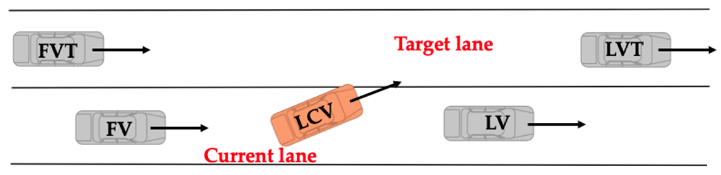
In the lane-changing scenario, five vehicles are involved (Figure 11): the lane-changing vehicle (LCV), the leading vehicle in the current lane (LV), the following vehicle in the current lane (FV), the leading vehicle in the target lane (LVT), and the following vehicle in the target lane (FVT). The LCV attempts to merge from the current lane into the target lane, influenced by the dynamic interactions with both the LV and FV in the original lane, as well as the LVT and FVT in the target lane. The relative positions, speeds, and accelerations of these vehicles significantly impact the success and safety of the lane-changing maneuver.

In mixed traffic flow, CAVs and HDVs are randomly distributed among the lane-changing vehicles and the target lane. To describe the impact of CAV degradation during lane-changing behavior, the following three typical lane-changing scenarios involving DCAVs have been selected for analysis, as shown in Figure 12.

4.4. Simulation

We conducted a simulation using a real road segment from the NGSIM traffic dataset. The objective was to evaluate the effectiveness of the total risk metric (R_total). We also assessed the impact of penetration rate, PRT, and lane-changing combinations on mixed traffic flow safety. Real driving data from 7:50 to 8:35 a.m. were used to simulate vehicle flow. This experiment aims to validate the content in Section 3.

The selected road segment is 640 m long, including entrance and exit ramps, as shown in Figure 5. The entrance ramp induces deceleration waves at the bottleneck, which propagate upstream and lead to rear-end collisions, as noted in previous studies [26]. The segment has limited lane-changing opportunities and a wide speed range (0 to 20 m/s), making it ideal for testing longitudinal and lateral safety behaviors. The first 50 m of the simulation serves as a warm-up and is not included in the analysis. The vehicle length l is 5 m. The car-following model parameters for IDM, CAV, and DCAV are shown in Table 4, Table 5, and Table 6, respectively.

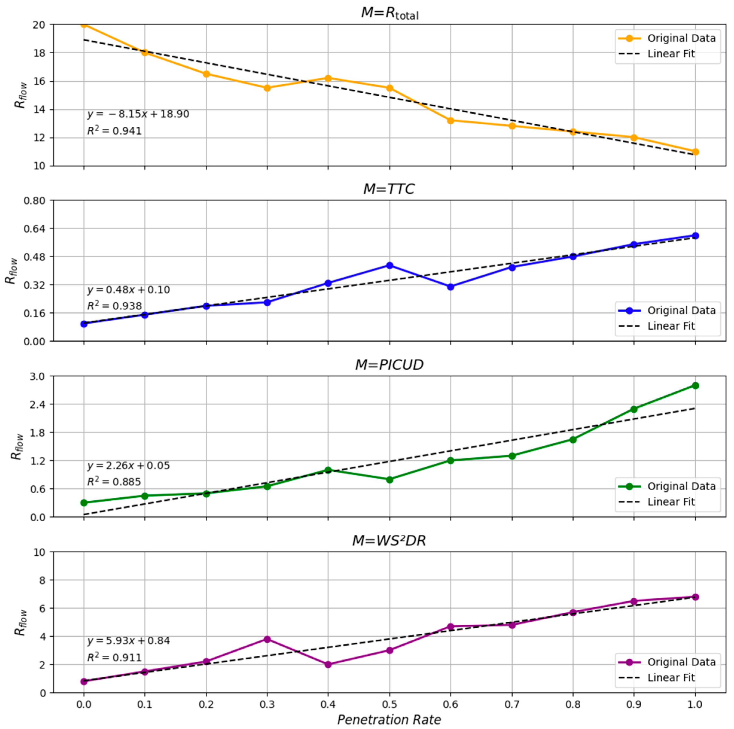
4.4.1. Effects of Penetration Rate of CAVs

A reduction in the penetration rate of CAV increases the probability of degradation phenomena. Additionally, the CAV penetration rate determines the proportion of the three types of vehicles within mixed traffic flows (see Section 4.1). Therefore, this part will focus on examining the impact of CAV penetration rate on collision risk (Figure 13).

From Figure 13, it can be seen that in the specific penetration rate range of 0.4–0.6, all four indicators exhibit fluctuations. Among them, R_total shows relatively sensitive changes. This is mainly because R_total takes into account both vehicle reaction time and CAV degradation, thereby better reflecting the overall traffic flow safety changes. In contrast, WS²DR shows significant fluctuations at a penetration rate of 0.4, while PICUD experiences a large fluctuation at 0.5. These findings indicate that vehicle behavior changes at these penetration rates have a more pronounced impact on traffic safety. On the other hand, the TTC indicator exhibits significant fluctuations later, at a penetration rate of 0.6. This suggests that TTC lacks responsiveness and fails to capture risk changes at medium to low penetration rates effectively. Compared to the other three typical SSMs, the absolute value of the linear model’s slope for R_total is the largest, indicating its higher sensitivity to changes in penetration rate. Additionally, its R² value is the highest, demonstrating that the variation trend of R_total is well-fitted by the linear model, exhibiting high stability and predictability.

This phenomenon suggests that at medium penetration rates (0.4–0.6), the increase in degraded CAVs and the complexity of vehicle interactions elevate safety risks in mixed-traffic environments. As the penetration rate continues to increase (above 0.6), a higher proportion of CAVs can better coordinate the flow, thereby reducing overall risk. Therefore, controlling the penetration rate within an appropriate range can balance the advantages of autonomous driving technology with the risks introduced by degradation, ultimately improving traffic safety.

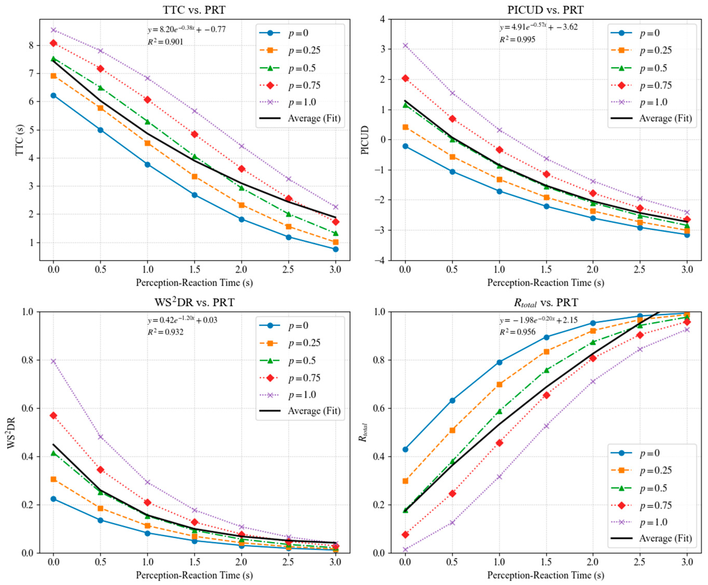
4.4.2. Effects of PRT

PRT significantly affects safety and risk levels in mixed traffic flows consisting of CAVs, DCAVs, and HDVs. In the following simulation, variations in PRT among different penetrations were taken into account, and the results are presented in Figure 14.

Figure 14 illustrates the impact of PRT on four different safety metrics, revealing the following findings:

(1)

When the penetration rate is 0.5, as PRT increases from 0 to 3 s, TTC, PICUD, and WS²DR decrease by more than 77%, while R_total increases by over 90%. This indicates that prolonged reaction times significantly elevate vehicle operational risks. At low PRT values (e.g., PRT = 0 s), the four metrics show significant differences between low penetration rates (p = 0 or p = 0.25) and high penetration rates (p = 0.75 or p = 1). However, at higher PRT values (e.g., PRT = 3 s), the gaps between the metric curves narrow, and the differences among the metrics diminish. This suggests that penetration rate has a greater influence when reaction time is short, while its impact decreases as PRT increases;

(2)

All metrics are notably influenced by the penetration rate. As the CAV penetration rate increases, the sensitivity of metrics to PRT decreases. At higher penetration rates (e.g., p = 0.75 or p = 1), the risk level stabilizes. This demonstrates that the cooperative control capabilities of CAVs effectively mitigate longitudinal and lateral risks caused by increased PRT;

(3)

The metrics vary in sensitivity and responsiveness to PRT changes. TTC has the steepest slope and the fastest change, making it suitable for short-term collision risk assessment. In contrast, R_total changes most gradually, making it more appropriate for assessing long-term comprehensive risks and macro-level trends;

(4)

The high correlation of the fitted curves (R² close to 1) confirms the exponential relationship between the metrics and PRT. R_total achieves the highest R² value (0.956), indicating superior explanatory power, applicability, and stability in reflecting the relationship between PRT and risk variations.

4.4.3. Effects of Lane-Changing Modes

To further analyze the impact of different lane-changing modes on traffic safety, we introduced Figure 15. This figure presents the variations in various safety metrics (TTC, WS²DR, PICUD, and R_total) under three degradation scenarios:

• Mode A: Degradation affects only the LCV.
• Mode B: Degradation affects only the FVT.
• Mode C: Degradation affects only the FV

In examining the variations of safety indicators across different lane-changing modes in Figure 15, we observe that Mode B consistently exhibits the lowest values of TTC and WS²DR, along with a negative PICUD, indicating the highest collision risk among the modes; Mode C, on the other hand, shows the highest TTC and WS²DR values and a positive PICUD, reflecting the lowest collision risk, while Mode A falls in between. R_total can arrive at the same conclusions as other metrics, demonstrating its ability to adapt to various risk scenarios.

These patterns occur because in Mode B, the degradation of the FVT increases its perception–reaction time and eliminates cooperative communication capabilities, preventing it from promptly detecting and responding to the LCV’s maneuvers, thereby elevating the likelihood of rear-end collisions. In Mode C, although the FV is degraded, the LCV is moving away from it during the lane change, allowing the FV sufficient time and space to react despite its increased reaction time, thus minimizing risk. Mode A presents a moderate risk because while the LCV’s degradation reduces its environmental perception accuracy, it retains control over its actions and can adopt conservative strategies to mitigate hazards; additionally, surrounding vehicles with full CACC functionality can adjust their behavior to compensate for the LCV’s limitations, reducing overall risk. Therefore, the dangerousness of these scenarios is ranked as Mode B > Mode A > Mode C.

By understanding these dynamics, traffic management systems can devise strategies to mitigate risks associated with increased PRTs and lane-changing maneuvers in mixed-traffic environments.

This study’s simulation analysis focuses on a specific road segment, providing valuable insights into mixed traffic safety. However, limitations exist. Simplified assumptions for PRT and lane-changing may not fully represent diverse driving behaviors in complex scenarios, affecting risk accuracy. Computational constraints limit the study to localized simulations, restricting scalability to larger networks. The lack of real-world validation also impacts reliability. Future research will incorporate diverse datasets, refine models, expand simulation scales, and integrate real-world data to enhance robustness and applicability.

5. Conclusions

The proposed risk assessment method effectively integrates car-following and lane-changing behaviors, offering a more precise evaluation of collision risks in mixed traffic flow. Empirical validation demonstrates that the method can effectively identify high-risk scenarios. The study reveals that the degradation effects of CAVs, PRT, and penetration rates have significant impacts on traffic safety, specifically in the following aspects:

(1)

When the TTC is set to 2 s, the collision risk threshold of R_total is determined to be 0.49, providing a reliable benchmark for identifying critical situations;

(2)

Considering CAV degradation, when the penetration rate of CAV is between 0.4 and 0.6, collision risks increase by an average of 15%, highlighting the safety challenges of intermediate CAV adoption rates in mixed traffic flow. R_total takes into account multiple factors, such as PRT, and demonstrates relatively sensitive variations, providing a more effective representation of overall changes in traffic flow safety;

(3)

At lower PRTs, penetration rates have a more significant impact on collision risks, whereas at higher PRTs, the impact decreases, as vehicle coordination is insufficient to mitigate the elevated risks caused by delayed PRTs. Compared to other metrics, R_total exhibits superior applicability and stability, making it more suitable for evaluating the long-term comprehensive risks and macro-level trends of traffic flow;

(4)

In lane-changing scenarios, the degradation of the FVT contributes the most to collision risks, emphasizing the importance of vehicle degradation location and its combinations in overall risk assessment.

This study offers practical recommendations for public traffic management, including the development of real-time risk prediction and warning systems to accurately identify high-risk car-following and lane-changing behaviors. It also suggests enhancements in lane management strategies and dynamic speed control measures, with a focus on addressing safety challenges in mixed traffic flows with intermediate CAV penetration rates. Special emergency response measures should also be established to mitigate risks arising from CAV degradation. Moreover, collaboration with vehicle manufacturers and traffic management agencies is essential to promote the deep integration of CAV technologies with transportation infrastructure, thereby enhancing overall traffic safety.

Future research should explore the real-time implementation of the proposed risk index within intelligent transportation systems and examine its effectiveness under different levels of vehicle automation and connectivity. Additionally, the applicability of this method should be extended to urban roads, intersections, and other complex traffic environments. Incorporating environmental factors, such as weather conditions and road surface quality, could further optimize the predictive capabilities of the model. Furthermore, dynamic risk thresholds and their integration with real-time control algorithms should be investigated to better support traffic safety management across diverse scenarios. These advancements will provide robust technical support for the global optimization and dynamic risk management of intelligent transportation systems.

References

1. Datler, B.; Harrer, M.; Jandrisits, M.; Ruehrup, S. The Road to Automation–Road Operators’ Challenges in the Introduction of Automated Driving. In Proceedings of the ITS World Congress, Montreal, QC, Canada, 29 October–2 November2017. [Google Scholar]
2. Li, S.; Anis, M.; Lord, D.; Zhang, H.; Zhou, Y.; Ye, X. Beyond 1D and oversimplified kinematics: A generic analytical framework for surrogate safety measures. Accid. Anal. Prev. 2024, 204, 107649. [Google Scholar] [CrossRef]
3. Mullakkal-Babu, F.A.; Wang, M.; Farah, H.; van Arem, B.; Happee, R. Comparative assessment of safety indicators for vehicle trajectories on highways. Transp. Res. Rec. 2017, 2659, 127–136. [Google Scholar] [CrossRef]
4. Wang, C.; Xie, Y.; Huang, H.; Liu, P. A review of surrogate safety measures and their applications in connected and automated vehicles safety modeling. Accid. Anal. Prev. 2021, 157, 106157. [Google Scholar] [CrossRef] [PubMed]
5. Tarko, A.P. Estimating the expected number of crashes with traffic conflicts and the Lomax Distribution–A theoretical and numerical exploration. Accid. Anal. Prev. 2018, 113, 63–73. [Google Scholar] [CrossRef]
6. Stipancic, J.; Miranda-Moreno, L.; Saunier, N.; Labbe, A. Surrogate safety and network screening: Modelling crash frequency using GPS travel data and latent Gaussian Spatial Models. Accid. Anal. Prev. 2018, 120, 174–187. [Google Scholar] [CrossRef]
7. Li, P.; Abdel-Aty, M.; Yuan, J. Using bus critical driving events as surrogate safety measures for pedestrian and bicycle crashes based on GPS trajectory data. Accid. Anal. Prev. 2021, 150, 105924. [Google Scholar] [CrossRef] [PubMed]
8. Arun, A.; Haque, M.M.; Bhaskar, A.; Washington, S.; Sayed, T. A systematic mapping review of surrogate safety assessment using traffic conflict techniques. Accid. Anal. Prev. 2021, 153, 106016. [Google Scholar] [CrossRef]
9. Oikonomou, M.G.; Ziakopoulos, A.; Chaudhry, A.; Thomas, P.; Yannis, G. From conflicts to crashes: Simulating macroscopic connected and automated driving vehicle safety. Accid. Anal. Prev. 2023, 187, 107087. [Google Scholar] [CrossRef]
10. Abdel-Aty, M.; Wang, Z.; Zheng, O.; Abdelraouf, A. Advances and applications of computer vision techniques in vehicle trajectory generation and surrogate traffic safety indicators. Accid. Anal. Prev. 2023, 191, 107191. [Google Scholar] [CrossRef]
11. Papadoulis, A.; Quddus, M.; Imprialou, M. Evaluating the safety impact of connected and autonomous vehicles on motorways. Accid. Anal. Prev. 2019, 124, 12–22. [Google Scholar] [CrossRef]
12. Sha, H.; Singh, M.K.; Haouari, R.; Papazikou, E.; Quddus, M.; Quigley, C.; Chaudhry, A.; Thomas, P.; Weijermars, W.; Morris, A. Network-wide safety impacts of dedicated lanes for connected and autonomous vehicles. Accid. Anal. Prev. 2024, 195, 107424. [Google Scholar] [CrossRef] [PubMed]
13. Tu, Y.; Wang, W.; Li, Y.; Xu, C.; Xu, T.; Li, X. Longitudinal safety impacts of cooperative adaptive cruise control vehicle’s degradation. J. Saf. Res. 2019, 69, 177–192. [Google Scholar] [CrossRef] [PubMed]
14. Qin, Y.; Wang, H.; Wang, W. Analysis on stability and safety for mixed traffic flow with connected auxiliary driving. Dongnan Daxue Xuebao (Ziran Kexue Ban)/J. Southeast Univ. (Nat. Sci. Ed.) 2018, 48, 188–194. [Google Scholar]
15. Yao, Z.; Hu, R.; Jiang, Y.; Xu, T. Stability and safety evaluation of mixed traffic flow with connected automated vehicles on expressways. J. Saf. Res. 2020, 75, 262–274. [Google Scholar] [CrossRef]
16. Li, Y.; Wang, H.; Wang, W.; Xing, L.; Liu, S.; Wei, X. Evaluation of the impacts of cooperative adaptive cruise control on reducing rear-end collision risks on freeways. Accid. Anal. Prev. 2017, 98, 87–95. [Google Scholar] [CrossRef]
17. Peng, G.; Huang, Y.; Tan, H. Phase transitions and congestion of heterogeneous lattice hydrodynamics model considering delayed difference feedback control in connected autonomous vehicles environment. Chaos Solitons Fractals 2024, 187, 115360. [Google Scholar] [CrossRef]
18. Hayward, J.C. Near Miss Determination through Use of a Scale of Danger; Highway Research Board: Washington, DC, USA, 1972. [Google Scholar]
19. Ozbay, K.; Yang, H.; Bartin, B.; Mudigonda, S. Derivation and validation of new simulation-based surrogate safety measure. Transp. Res. Rec. 2008, 2083, 105–113. [Google Scholar] [CrossRef]
20. Uno, N.; Iida, Y.; Itsubo, S.; Yasuhara, S. A microscopic analysis of traffic conflict caused by lane-changing vehicle at weaving section. In Proceedings of the 13th Mini-EURO Conference-Handling Uncertainty in the Analysis of Traffic and Transportation Systems, Bari, Italy, 10–13 June 2002; pp. 10–13. [Google Scholar]
21. Hou, K.; Zheng, F.; Liu, X. Enhancing mixed traffic safety assessment: A novel safety metric combined with a comprehensive behavioral modeling framework. Accid. Anal. Prev. 2024, 208, 107766. [Google Scholar] [CrossRef]
22. Wen, X.; Cui, Z.; Jian, S. Characterizing car-following behaviors of human drivers when following automated vehicles using the real-world dataset. Accid. Anal. Prev. 2022, 172, 106689. [Google Scholar] [CrossRef]
23. Kesting, A.; Treiber, M. How reaction time, update time, and adaptation time influence the stability of traffic flow. Comput.-Aided Civ. Infrastruct. Eng. 2008, 23, 125–137. [Google Scholar] [CrossRef]
24. Milanés, V.; Shladover, S.E. Modeling cooperative and autonomous adaptive cruise control dynamic responses using experimental data. Transp. Res. Part C Emerg. Technol. 2014, 48, 285–300. [Google Scholar] [CrossRef]
25. Li, R.; Sun, S.; Wu, Y.; Hao, H.; Wen, X.; Yao, Z. Fundamental diagram of mixed traffic flow considering time lags, platooning intensity, and the degradation of connected automated vehicles. Phys. A 2023, 627, 129130. [Google Scholar] [CrossRef]
26. Hou, K.; Zheng, F.; Liu, X.; Guo, G. Cooperative on-ramp merging control model for mixed traffic on multi-lane freeways. IEEE Trans. Intell. Transp. Syst. 2023, 24, 10774–10790. [Google Scholar] [CrossRef]
Figure 1. The flowchart of methodology.
Applsci 14 11400 g001
Figure 2. Sensitivity Analysis of Rlon.
Applsci 14 11400 g002
Figure 3. Sensitivity Analysis of Rlat.
Applsci 14 11400 g003
Figure 4. Sensitivity Analysis of Rtotal.
Applsci 14 11400 g004
Figure 5. Schematic diagram of the US-101 detection section.
Applsci 14 11400 g005
Figure 6. Data smoothing results. (a) Position smoothing result of Vehicle ID56; (b) speed smoothing result of Vehicle ID 56; (c) acceleration smoothing result of Vehicle ID 56.
Applsci 14 11400 g006aApplsci 14 11400 g006b
Figure 7. Evaluation results of different vehicles. (a) Evaluation results of vehicle ID 63; (b) evaluation results of vehicle ID 361; (c) evaluation results of vehicle ID 1109; (d) evaluation results of vehicle ID 1342.
Applsci 14 11400 g007aApplsci 14 11400 g007b
Figure 8. Kendall’s Tau coefficient matrix of SSMs.
Applsci 14 11400 g008
Figure 9. Relationship between TTC and other SSMs.
Applsci 14 11400 g009
Figure 10. The degradation phenomenon of CAV.
Applsci 14 11400 g010
Figure 11. Lane-changing scenario.
Applsci 14 11400 g011
Figure 12. Impact of CAV degradation in lane-changing. (a) Degradation of LCV (LCV transforms into LCV’); (b) degradation of FVT (FVT transforms into FVT’); (c) degradation of FV (FV transforms into FV’).
Applsci 14 11400 g012
Figure 13. Impact of penetration rate on various safety metrics.
Applsci 14 11400 g013
Figure 14. Impact of PRT on various safety metrics.
Applsci 14 11400 g014
Figure 15. Impact of lane-changing modes on various safety metrics.
Applsci 14 11400 g015