Abstract
The Sumatran Fault runs from the southeast (SE) to the northwest (NW) of Sumatra Island, with the highest slip rates reaching about 3.0 cm per year in the northwestern part. There is a seismic gap along this fault, including the northern Aceh domain, which consists of the Aceh and Seulimeum fault segments. Previous studies have used various methods to investigate the Sumatran Fault system, including seismic, geoelectric, gravity anomaly, and magnetotellurics (MT). The MT method has proven advantageous as it can non-destructively image a wide range of depths. However, previous studies using the two-dimensional (2D) MT inversion did not represent realistic information of the subsurface conditions. Therefore, a three-dimensional (3D) MT data inversion was used in this study to obtain more realistic information about the resistivity structure of the Aceh and Seulimeum segments. The results confirmed that the Sumatran Fault is a strike-slip fault, with a relatively northwest (NW)–southeast (SE) direction of conductivity strike with an angle of S 71.61° E from Groom–Bailey decomposition of MT data. The 3D resistivity distribution model from 33 stations showed that the Aceh Fault Segment is 20–30 km away, while the Seulimeum Fault Segment is 55–60 km away based on the MT data. The results also indicated a creeping zone at a depth of 2 km beneath the Aceh Fault Segment. Different rock formations were identified beneath the fault system, with the western part of the Aceh Segment dominated by high-resistivity metamorphic rocks (150–1000 Ωm) from the Triassic–Cretaceous age. The zone between the Aceh and Seulimeum fault segments exhibited low resistivity, characterized by volcanic rocks (1–15 Ωm) from the Lam Teuba Volcanic Formation and the Indrapuri Formation. Beneath the eastern part of the Seulimeum Fault Segment was found to consist of low-resistivity quaternary volcanic rocks (1–15 Ωm) and high-resistivity andesite rocks (4.5 × 10⁴–1.7 × 10⁵ Ωm). These findings correlated well with the geological map.
1. Introduction
Sumatra Island is situated at a plate boundary in the subduction zone between the Indian and Australian plates, with the Sundaland plate overriding. The Indian Ocean plate moves towards the north–northeast (NNE) at a relative rate of 7.7 cm a−1, leading to oblique subduction at a 45° angle at the Sunda Trench. Based on the MORVEL model, slip rates of the subduction between the Indian and the Sundaland plates are 46–48 mm per year off Sumatra Island [1]. Because of the oblique subduction, the trench-parallel strike-slip fault was formed on the southwestern coast of Sumatra Island [2]. Sumatran Fault was created due to the oblique subduction process of the Indo-Australia plate beneath the Eurasian plate [3,4,5,6]. It stretches for 1900 km from 10° N to 7° S and has 19 major fault segments [7]. Apart from being a trench-parallel strike-slip fault in an oblique subduction system, the Sumatran Fault is also part of a volcanic arc [8].
A seismic creep down has been identified in the northern segment of the Sumatran Fault. It occurs at a depth of 7.3 ± 4.8 km with a rate of 2.0 ± 0.6 cm per year [9]. This slip rate is higher than that of the southern segment of the Sumatran Fault, which has an estimated locking depth of 14.8 ± 3.4 km with a slip rate of 1.6 ± 0.6 cm per year [9]. Despite the shallow creep, the estimated width of the locked zone is 9.4 ± 6.4 km in the northwestern part of the Sumatran Fault zone. These findings indicate that the northern segment has the potential to cause earthquakes with a magnitude of 7 [9]. Geological estimates of slip rates on the Sumatran Fault increase from southeast to northwest, with the maximum rates reaching about 3.0 cm per year in the northwestern part of Sumatra Island [7,10,11,12,13]. The Sumatran Fault also has a seismic gap for earthquakes with historical earthquakes of a magnitude of M ≥ 7. This gap includes the northern Aceh domain, which consists of the Aceh and Seulimeum segments in northwestern Sumatra Island. This information was reported in a historical observation of seismicity [7,14]. High slip rates, the presence of locking zones, and seismic gaps on the northern segment of the Sumatran Fault, which includes the Aceh and Seulimeum segments, are of serious concern to researchers and continue to be studied by various related scientific fields, including the geophysics.
One of the geophysical methods that can be used to study fault structures that are generally relatively deep is magnetotellurics. Magnetotellurics (MT) is a passive geophysical exploration method based on electromagnetic induction and it uses the natural variations in the Earth’s magnetic and electric fields as a source. These variations are caused by the interaction of solar wind with the magnetosphere and ionosphere, as well as by thunderstorm activity in equatorial regions [15,16]. Alternating currents that are induced in the rocks provide information about the Earth’s structure. The direction and strength of these currents depend on the electrical conductivity distribution [17]. Analyzing the relationships between the values of respective electromagnetic field components recorded at the surface allows us to determine the subsurface electrical conductivity [18]. The MT method has been widely used for the study of fault investigation [19,20,21,22].
Previous studies about the Sumatran Fault using the MT method have been performed by characterizing a model of 2D MT inversion, using an algorithm developed by Ogawa and Uchida [23]. The results show that there is a contrast resistivity which characterizes the structure of the Sumatran Fault. The shallow part just beneath the contrast resistivity is characterized as the locked zone at a depth of 15 km in the form of the resistive zone, while at a depth of 20 km, it is characterized as a melting zone [24]. Other studies about the Sumatran Fault have been performed using 2D gravity data modeling along with the Aceh and Seulimeum fault segments in the NW-SE direction, which showed that at the distance of 25–50 km, Aceh segment faults had been identified, characterized by two different vertical blocks densities. In addition, at a distance of 50–75 km, the Seulimeum Fault Segment has been identified, which is shown by two vertical blocks of relatively high and low densities [25]. The other study about the electrical resistivity distribution of the Seulimeum Fault Segment System was also performed using the geoelectrical method [26]. The study revealed that the Seulimeum Fault System consists of a horst and graben system. The depth of the Seulimeum Segment increases from 20–50 m in the southern part to 50–200 m in the northern part as it approaches the Andaman Sea. A conductive zone characterizes the graben, while the horst is characterized by a resistive zone [26]. In this study, a three-dimensional (3D) MT data inversion was used to investigate and confirm more realistic information about the resistivity structure of the Aceh Segment Fault and the Seulimeum Segment Fault to better understand the fault characteristics associating hazards with the fault, considering that these segments have the potential for seismic activity in the form of earthquakes with magnitude [14,27].
2. Geological Setting
Sumatra, one of the large islands in the Indonesian archipelago and the fifth largest in the world, covers an area of 473,606 km2. It extends 1760 km from northwest (NW) to southeast (SW) and is 400 km wide. Sumatra includes the Mentawai Islands from Simeulue to the Pagai Islands, Enggano Island, and Tin Island, which comprises the Bangka, Belitung, and Riau Islands to the east. The Bukit Barisan Mountain range runs parallel along Sumatra’s southwest coast, serving as the backbone of the main island [28]. Sumatra is situated at a plate boundary where the Indian and Australian plates are pushed underneath the Sundaland plate. This oblique subduction has caused the formation of a trench-parallel strike-slip fault near the southwestern coast of Sumatra Island, known as the Sumatran Fault [2]. The fault accommodates most of the lateral motion of the 7 mm/year oblique convergence between the Indo-Australia and Eurasian plates at the Sunda subduction system [5,29]. The total length of the right-lateral strike-slip Sumatran Fault is 1900 km long, divided into 19 major segments based on second-order geometric irregularities. These segments include Sunda, Semangko, Kumering, Manna, Musi, Ketaun, Dikit, Siulak, Suiliti, Sumami, Sianok, Sumpur, Barumun, Angkola, Toru, Renun, Tripa, Aceh, and Seulimeum [7]. Furthermore, based on the geometry and detailed structure of the Sumatran Fault, the forearc basin, outer-arc ridge, and volcanic arc, Sumatra is divided into northern, central, and southern domains [7]. Based on paleontological evidence surveys regarding the age of stratigraphic units in Sumatra, it has been shown that the fossil rock units in the subsurface pre-tertiary layers of Sumatra range in age from early Carboniferous to mid-Cretaceous [28,30]. The basement rocks of Sumatra are categorized into northern, central, and southern parts according to their stratigraphic ages: Pre-Carboniferous basement, Carboniferous–Early Permian, Mid–Late Permian, Mid–Late Triassic, and Jurassic–Mid-Cretaceous. In the northern domain, there are three segments of the Sumatran fault: the Aceh and Seulimeum faults in the north section and the Tripa Fault in the southern section [8].
These map quadrangles cover the fault of the Aceh Segment, Banda Aceh [13], and Takengon or Meulaboh [31], which is documented by the Geological Survey Agency of Indonesia and is published in several regional geology maps at 1:250,000 scale. They provide information about the geology of the Aceh Segment Fault, which is given in Figure 1. The Aceh Fault Zone is western Indonesia’s northernmost segment of the Sumatran Fault System. It spans 250 km and passes through three districts: West Aceh, Pidie Jaya, and Aceh Besar. The fault segment is divided into seven sub-segments: Beutong, Kuala Tripa, Geumpang, Mane Jantho, Indrapuri, and Pulo Aceh. Each sub-segment varies in length from 15.7 to 50 km and shows right-lateral strike-slip fault kinematics [32]. The Aceh Segment Fault continues offshore of the Andaman Sea and has a dip angle of 12°–17° [33]. The northwestern section of the Aceh Segment Fault passes through the low relief region of Banda Aceh. It continues offshore and merges with the Andaman Nicobar Fault [29,34]. The northern section of Aceh Segment Fault separates high- and low-relief areas, while its southern section crosses the mountainous zone [7]. The high-relief areas are dominated by basement rocks composed of Trias–Cretaceous age metamorphic rocks and igneous rocks with partially Mesozoic sedimentary and Miocene and Quaternary volcanic rocks [6,32]. The low relief areas are filled with young alluvium deposits composed of silt (gravel sediment) [35]. In the low relief area, the Indrapuri Formation comprises older terrace deposits, partly volcanic gravels, sands, and marine/continental sedimentary, as shown in Figure 1. The stratigraphic of those rocks is shown in Figure 2.
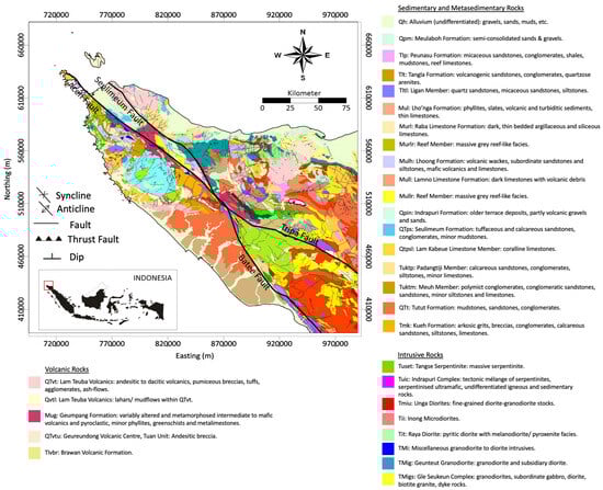
Figure 1.
A geological map of the study area and surroundings [13,31].
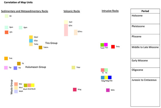
Figure 2.
Rock stratigraphy of the study area and surroundings [13,31].
The fault of the Seulimeum Segment stretches from the Seulawah Agam volcano. It continues onshore to Sabang Island [36], where the depth increases from the southern part (20–50 m) to the northern part (50–200 m) when approaching the Andaman Sea [26]. The Seulimeum Segment lies east of and branches northward from the Aceh Segment, where the southeastern end of the Seulimeum Segment is located ~4 km to the northeast of the Aceh Segment [35]. The length of this segment is 120 km [7,33]. The Seulimeum Segment is identified as a strike-slip fault similar to the Sumatran Fault System characteristics, which is known to be much more active in the region of the bifurcation of the Aceh Segment and the Seulimeum Segment based on the seismological data [37]. Based on the geological map as shown in Figure 1, the Seulimeum Segment is dominated by Quaternary volcanic rocks, which include the Lam Teuba Volcanic Formation composed of andesitic to dacitic volcanic, pumiceous breccia, tuffs, agglomerate, and ash flows. The Seulimeum Segment also consists of intruded ash, composed of tuffaceous and calcareous sandstones, conglomerates, and minor mudstones [13]. The structure of the Seulimeum Segment breaks into two sections, which produce a horst and graben system, indicating the fault system from the moving plat [26].
3. MT Method
3.1. MT Method Theory
The MT method is a passive geophysical exploration that uses the electromagnetic concept to measure the variation in the natural electric field E and the magnetic field H at the surface to provide information about resistivity at the Earth’s subsurface. The theory of the MT method was first introduced by Tikhonov [16] and detailed by Cagniard [15] and Wait [38]. The penetration depth of the electromagnetic wave in the Earth’s subsurface depends on the period of the electromagnetic sounding and conductivity of the Earth’s structure, which has been known as skin depth δ and is given in this Equation (1) [15]
with T as the period and as the apparent resistivity obtained from the impedance tensor of MT data. The ratio of electric field and magnetic field is known as an impedance tensor Z, known as the transfer function of the MT, which is given by Equations (2) and (3) [38]
The basic information about vertical variations in the conductivity is given by the off-diagonal components Zxy and Zyx. While the diagonal components Zxx and Zyy of the MT impedance tensor indicate the asymmetry of the medium, and they become zero if the medium is symmetric about a vertical plane passing through the observation site [39]. MT data can be expressed as apparent resistivity (Equation (4)) and phase (Equation (5)) [15,16,38].
where is the apparent resistivity (Ωm), is the permeability, is the frequency, Z is the impedance, and is the phase.
3.2. MT Data Acquisition and Processing
MT data were recorded in the northern domain of Aceh using MTU-5A units manufactured by Phoenix Geophysics Ltd., Toronto, ON, Canada, with 33 total stations spread out as shown in Figure 3. All the data recorded include five components of the time-varying electromagnetic field, which comprises two components of electric field , two components of horizontal magnetic field , and one component of vertical magnetic field . In data acquisition, MT stations can be grouped into 4 lines based on the similarity of data acquisition, namely Line A, Line B, Line C, and Line D (Table 1). The frequency measurement ranged from 320 to 0.05 Hz.
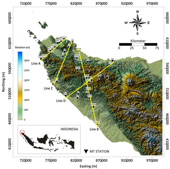
Figure 3.
The distribution of MT stations (black triangle) at the northern Aceh research site, which is divided into 4 lines (yellow line) based on data acquisition time into Line A (October and November 2008), Line B (August 2009), Line C (July–August 2012), and Line D (July–August 2012).

Table 1.
Description of line, acquisition time, line direction, and site name.
The first step involves preprocessing the time series data (TS3, TS4, TS5), where the data are grouped based on the duration of data collection. Next, noise peaks are removed from the recorded electric field data, and corrections are made to the recorded electric field data. Then, the MT time series data were transformed into the frequency domain using Fast Fourier Transform (FFT) and filtered using robust processing [40,41], producing results in MTH and MTL files using SSMT 2000 software. To choose good and bad data, we used MT-corrector software v.5.6.0.0 (Nord-West Ltd., Moscow, Russia), which used cross-power (smoothing) XPR analysis and the dispersion relation (DR) concept, which provides a more intuitive insight into how data should be corrected [42]. The dispersion relation constrained the cross-power selection is written in Equation (6) [43]
where is the impedance phase, is the frequency, is the apparent resistivity, and is 1/.
The smoothness property of the MT curve data was validated using smoothing splines for robust estimation [39]. The data were then smoothed by cubic spline interpolation. The unknown constants for correcting data were solved by automatically fitting the calculated curves to the corresponding real part (log amplitude) spline using dispersion relation constraint [42]. Dispersion relation (DR) in post-processing MT detects and eliminates noisy/biased MT data [18]. It is an efficient quality assessment tool for MT data at broadband frequencies [42]. The result of post-processing data using cross-power XPR analysis and smoothing using DR was reported to produce smoother resistivity response curves with smaller error bars compared to processing without using DR, especially at low frequencies, as shown in Figure 4. Figure 4a,c,e shows the cross-power XPR analysis and smoothing without the concept of DR. In contrast, Figure 4b,d,f shows the cross-power XPR analysis and smoothing with the DR concept. The result of the post-processing is found in the form of an EDI file, which provides information about impedance, apparent resistivity, phase, and the tipper parameter.
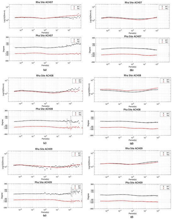
Figure 4.
Examples of data processing for ACH07, ACH08, and ACH09 stations on Line A: (a,c,e) MT data after cross-power XPR analysis and smoothing without using DR concept and (b,d,f) MT data after cross-power XPR analysis and smoothing using DR concept. (Rha for apparent resistivity and Pha for phase, while the black dot is XY polarization and the red dot is YX polarization).
3.3. Dimensionality Analysis
Dimensionality analysis of MT data is important to identify the Earth’s subsurface geometry characteristics by utilizing the information in the impedance tensor [39]. Some of the dimensionality analysis is performed by using a polar diagram, induction arrows [39], tipper magnitude [36], and phase tensor [44]. A polar diagram is a diagram that depicts the dependency of the impedance tensor on the strike direction [45,46,47]. The off-diagonal components of the impedance tensor given by Equation (3) represent several parameters of MT data, including a polar diagram and phase tensor. By rotating Equation (3) with rotation operator R (Equation (7)), Equation (8) can be rewritten:
where is the rotation angle. Then, we obtain each component of the impedance tensor Z, and its results can be given as Equations (9) and (10) [39]:
with , , and given by Equations (11)–(13):
Because the angle varies from 0 to 2, the tips of the resultant segments show closed curves called impedance polar diagrams. The components of and are known as the amplitude polar diagrams. At the same time, the component of is known as the phase polar diagram. They may form an oval, figure of eight, or a flower with four petals. In the case of a one-dimensional model (1D model), the polar diagram for reduces to a point. In contrast, the polar diagrams for and are circles of radius and , respectively. In the two-dimensional Earth model (2D model), the diagram of forms a flower with four identical petals. The bisectors between these petals are oriented in the longitudinal and transverse directions. The diagrams of and are ovals. The major and minor diameters of them, , , and , , are longitudinally and transversally directed. In the three-dimensional Earth model (3D model), the polar diagram is distorted and forms a peanut shape because of the asymmetry of the medium [18].
The next dimensionality analysis is induction arrows, which qualitatively indicate the location of the induction field. The transfer function between the vertical and the horizontal magnetic field, as shown in Equation (3) is used to determine induction arrows [48]. Inductions arrows represent a geomagnetic transfer function that consists of two dimensionless real vectors, as is shown in Equations (14) and (15):
where Tx is the x-component of the tipper vector, Ty is the y-component of the tipper vector, represents real part of the tipper vector, and represents an imaginary part of the tipper vector. The tipper vector is the vector that express the relationship between the horizontal magnetic field and vertical magnetic field , and it can be mathematically expressed as Equation (16):
Induction arrows are used to represent the geomagnetic transfer function and to identify the presence of lateral conductivity variations. They are an alternative form of the tipper [39] since the vertical magnetic field is produced by the lateral conductivity gradient [17]. There are two conventions for representing induction arrows: the Parkinson convention, where the tipper vector arrows point to the conducting body [49], and the Wiese convention, where the tipper vector arrows point away from the conducting body [50].
3.4. Three-Dimensional MT Inversion
The 3D inversion is used to perform the information about the resistivity distribution of the Earth’s subsurface by generating the Earth model. Three-dimensional inversion algorithm that is used in this study employs ModeEM software (https://www.mtnet.info/main/source.html (accessed on 1 June 2022)) [51,52]. The ModeEM 3D inversion code was used to create a 3D model of the geoelectric structure through gradient-based minimization of the objective function as Equation (17) [52]:
with Cd as the covariance of data errors, f(m) as the forward mapping, d as a data vector, m as an M-dimensional Earth conductivity model parameter vector, Cm as the model covariance, as the damping parameter, and m0 as the prior model. The algorithm of the ModeEM software uses a gradient-based optimization algorithm such as the Nonlinear Conjugate Gradient (NLCG) with minimal structure to minimize the objective function, which is solved by the Data-Space Conjugate Gradient Scheme (DCG) solver. The NLCG was designed to minimize the difference between the modeled and observed data. Using the NLCG approach, the gradient of Equation (17) with respect to variations in model parameters m must be evaluated, as shown in Equation (18):
where J is the sensitivity matrices, mn is a n-th of m, r is the data residual that is represented by , and f(m) is the n-th forward mapping. The gradient is then used to calculate a new ‘conjugate’ search direction in the model space.
The NLCG also essentially uses the same basic computational steps as required for solving the linearized equation [52]. The search for minimization error in the NCLG of the ModeEM software is based on a quadratic approach. If the solution does not fulfill the reduction conditions, then backtracking of the minimal error will use cubic interpolation. This step only needs one gradient evaluation, which is quite efficient for computation. The NLCG also implements automatic criteria to reduce the damping parameter () when the convergence stops [51]. This makes the ModeEM software more efficient for use. Using the DCG, the linearized objective function in Equation (17) transforms into that shown in Equation (19) [51]:
The model parameter update is computed by Equation (20) [51]:
where is the boundary condition, and J is the sensitivity matrices.
The electrical resistivity of the Earth’s subsurface structure is characterized by electromagnetic field components measured at the Earth’s surface using a transfer functions relationship. Inversion is used to obtain the actual resistivity distribution of the Earth’s subsurface in the form of the resistivity model. Electrical resistivity is a crucial physical property of rocks that aids in distinguishing geological formations with different petrophysical characteristics. The range of electrical resistivity varies from fractions of in sedimentary rocks to hundreds of thousands of in crystalline rocks [53,54,55]. The electromagnetic transfer function of the impedance tensor (Z), used in this study to characterize the electrical resistivity structure, is visualized as a quality in terms of apparent resistivity and phase. The impedance from 34 stations was used for inversion input. Logarithmic frequencies ranging from 320 Hz to 0.1 Hz were selected. The important parameters that were selected before starting the inversion were a mesh orientation, the starting model, and the smoothing parameters (covariance) because the modeling results were affected by the choice of those parameters [56]. In this study, the inversion grid consists of 63,360 cells (48 × 44 × 30 cells), and the area of interest (AOI) consists of 38 × 34 cells of 5 × 5 km horizontal size, as is shown in Figure 5. The size of 5 × 5 km for each cell was chosen based on the MT station spacing in a field that is approximately around 6–20 km so that each station can be represented by the model. If the cell size was reduced, the total number of cells would increase, and then the computation time would increase significantly considering the distance between stations, which is approximately above 6 km [57]. In addition, when the cell size is reduced to less than 5 km, the interpolation of the MT data inversion results for each station cannot be connected between one station and another because the MT data distance is above 6 km. The vertical cell increment is 500 m from the surface to 5 km of the model AOI, which consists of 10 cells. After 5 km, the range of vertical model cells grows logarithmically with an incremental factor of 1.2. The starting model we used as a prior model was homogenous with a 100 value of the resistivity, which was selected based on the reference [51]. The total number of NLG iterations, which were used to reduce the nRMS value from 24.532 to 7.138, was 26 iterations. The inversion running time was four days. It was recorded that each iteration takes 3–4 h.
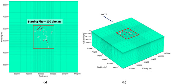
Figure 5.
(a) Planar view of the mesh for the inversion and (b) 3D view of the mesh for inversion, which were used in this research (the red box is the AOI which includes all the MT stations, and Rho is the model resistivity). The black triangles depict the MT station.
4. Results
4.1. Dimensionality Analysis: Polar Diagram
This study utilized dimensionality analysis through polar diagrams and induction arrows. The polar diagram was plotted at different frequencies, indicating shallow to deep skin depths, respectively, 317 Hz, 100 Hz, 10 Hz, 1 Hz, 0.1 Hz, and 0.05 Hz, as shown in Figure 6. Observing Figure 6a and comparing it to the reference [39], we found that at the high frequency of 317 Hz, the absolute value of the polar diagram component, represented by , displayed a dominated flower petal shape, indicated in red. Meanwhile, the absolute value of the polar diagram component exhibited a dominated circular shape, shown in black, reflecting the characteristics of the Earth model transitioning from 1D to 2D model. Some stations at the frequency of 317 Hz have an asymmetric flower petal shape for the component and a peanut shape for the component in C1, SARP, MANE, and D1 station, indicating a 3D model. At station D8, the characteristics of a 1D Earth model were depicted with no absolute value for the component in the polar diagram, and a circular shape for the absolute value of the component.
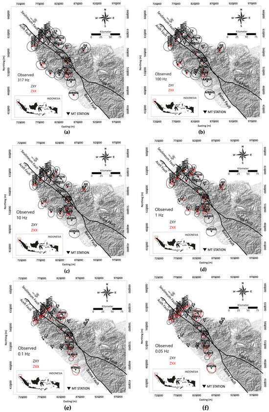
Figure 6.
Polar diagram for the frequencies of (a) 317 Hz, (b) 100 Hz, (c) 10 Hz, (d) 1 Hz, (e) 0.1 Hz, and (f) 0.05 Hz. The black triangle is the MT station, the red diagrams depict , and the black diagrams depict .
In Figure 6b, at a frequency of 100 Hz, the absolute value of the symmetric flower petal shape dominates the absolute value component. The absolute value of the component is dominated by a circular shape. This indicates a transition from a 1D to a 2D Earth model. However, certain stations (ACH2, MNYK, C1, D1, D4, and D7) exhibit a 3D asymmetric flower petal shape for the component and a peanut shape for the component. The C3, KEMA, and KAWA stations depict 1D geometric characteristics with no component in the polar diagram, and a circular shape for the component.
In Figure 6c at a frequency of 10 Hz, the polar diagram component shows an asymmetric flower petal shape, while the component displays a peanut shape. This indicates a 3D Earth model geometry at stations ACH02, GEM, MNYK, MANE, C2, D1, D2, and D7. On the other hand, stations the KAWA, KEMA, and MBMG represent a 1D Earth model geometry as the component (red) is absent, and the component (black) is circular. The rest of the stations depict a 2D geometry shown by a symmetric flower petal shape for the component and an elliptical shape for the component.
In Figure 6d, at a frequency of 1 Hz, the component is predominantly an asymmetric flower petal shape. In contrast, the component (black) is predominantly a peanut shape across all stations in Line D (D1, D2, D3, D4, D5, D7, and D8). This pattern is observed in most stations in Line A (ACH02, ACH04, ACH05, and ACH09), most stations in Line C (C2, C5, and C6), and the central part of Line B (SARP, MNYK, and MANE). No station shows 1D geometric characteristics.
In Figure 6e, at a frequency of 0.1 Hz, most stations in Line A show the characteristics of a 3D Earth model geometry. This is shown by the component (red) having an asymmetric flower petal shape, and the component (black) having a peanut shape. The stations exhibiting these characteristics are ACH01, ACH02, ACH04, ACH05, ACH06, ACH07, PIDIB, MANE, KAWA, SARP, C3, and D4. Note that other stations could not depict these characteristics due to data limitations.
In Figure 6f at a frequency of 0.05 Hz, the entire stations of Line A (ACH01, ACH02, ACH04, ACH05, ACH06, ACH07, and ACH08 station) are characterized by an asymmetric flower petal shape for the component (red) and a peanut shape for the component (black), indicating a 3D Earth model. The stations PIDIB, KAWA, SARP, D4, MANE, and GEM also depict a 3D Earth model. Other stations cannot be depicted due to data limitations. It can be concluded that the polar diagram pattern increasingly reflects a 3D Earth model as the frequency decreases, showing the deeper skin depth, as shown in Figure 6.
4.2. Dimensionality Analysis: Induction Arrows
In Figure 7, based on the Parkinson convention, low-resistivity zones (conductive zones) are represented by red arrows for the real component of induction and blue arrows for the imaginary component. At a frequency of 317 Hz, as shown in Figure 7a, the induction arrows point towards conductive zones from the northwest (NW) to the southeast (SE). The stations ACH04, ACH05, and C3 show arrows pointing from the southwest (SW) to the northeast (NE) in the northwest part, while the stations ACH06, ACH07, ACH08, ACH09, ACH10, ACH11, and C4 display arrows pointing from NE to SW, indicating a conductive zone along the NW-SE direction. Similarly, the stations C5 and KEMA point to conductive zones towards the SE and NW, respectively. Additionally, the ACH02 station shows a conductive zone towards the SE, and the SARP station indicates a conductive zone towards the NW. In the southeast part, the stations D1, D4, D7, D8, TANG, and GEM show arrows pointing from NE to SW, indicating a conductive zone along the NW-SE direction. The presence of the Aceh Fault extending along the NW-SE direction is identified as the conductive zones extending from NW to SW based on the references [7,58], which is shown by the red pointing arrows. However, some stations, such as ACH01, C1, and MBMG, show a different direction from the NW-SE path, which points towards SW. This is due to the influence of conductivity from the sea [59]. On the other hand, the induction arrows of the KAWA station point east (E), and are associated with the Batee Fault located in the southeast.
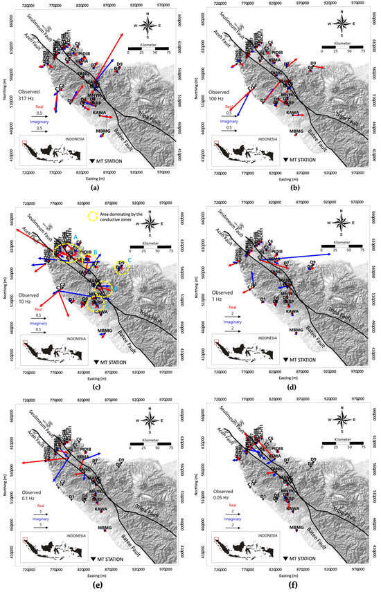
Figure 7.
Induction arrows for frequencies of (a) 317 Hz, (b) 100 Hz, (c) 10 Hz, (d) 1 Hz, (e) 0.1 Hz, and (f) 0.05 Hz in the different scale of induction arrows. The red arrows depict the real part of the tipper vector and the black diagrams depict the imaginery part of tipper vector (using Parkinson convention, red arrows point to the conducting body). The A, B, C, D, and E (yellow circle) depict dominant conductive zones.
At a frequency of 100 Hz, the pattern in Figure 7b is almost the same as at 317 Hz. The induction arrows generally point towards conductive zones extending from NW to SE. The direction of the induction arrows at each station remains the same, but some stations have longer length components of the induction arrows. The length of the induction arrows is determined by the amplitude of the real component. A larger real component is usually observed in coastal areas [59], as seen at the stations ACH01, C1, MBMG, and D9. At this frequency, some stations experience rotation. For instance, the C1 station changes direction from SW to W due to the influence of sea conductivity [59]. The MANE station experiences a shortening of the induction arrows, indicating a decrease in amplitude. This suggests that at a depth corresponding to the 100 Hz frequency, the conductivity effect of the nearby conductive zone is more influential than the sea conductivity effect.
In Figure 7c, at a frequency of 10 Hz, the conductive zones are generally localized, indicated by the presence of conductive zones marked with dashed circles in areas A, B, C, D, and E. Conductive zone A is confirmed due to the presence of the Aceh Fault and the Seulimeum Fault on the geological map in Figure 1. Conductive zone B, consisting of the stations PIDIB, KEMA, and TANG, points to alluvial sediments with conductive resistivity ranging from 10 to 800 Ωm on the geological map in Figure 1. Zone D indicates a conductive zone towards the SE, aligning with the direction of the Aceh Fault. Zone E indicates a conductive zone influenced by alluvial sediments in the SW, with conductive resistivity ranging from 10 to 800 Ωm on the geological map in Figure 1. On the other hand, in Figure 7d–f at frequencies of 1 Hz, 0.1 Hz, and 0.05 Hz, respectively, they have the same pattern as the other high frequencies, such as 317 Hz and 100 Hz.
In Figure 8a–f, the induction arrows are shown at the same scale of 0.5. They show that as the period increases (frequency decreases), the sea conductivity begins to affect the stations far from the coastal area [59]. This is as the induction arrows of some stations that are located far from the coastal area begin to have longer arrows pointing towards the sea at frequencies of 0.1 Hz and 0.05 Hz, as shown in Figure 8e,f. On the other hand, some stations at those frequencies do not have available data, leading to a lack of induction arrow information for the stations C1, C2, C3, C4, C5, C6, D1, D2, D3, D4, D5, D6, D7, and D8. Based on the induction arrows shown in Figure 7a–f and Figure 8a–f, the strike direction which is characterized by a conductive zone was shown along the NW-SE direction.
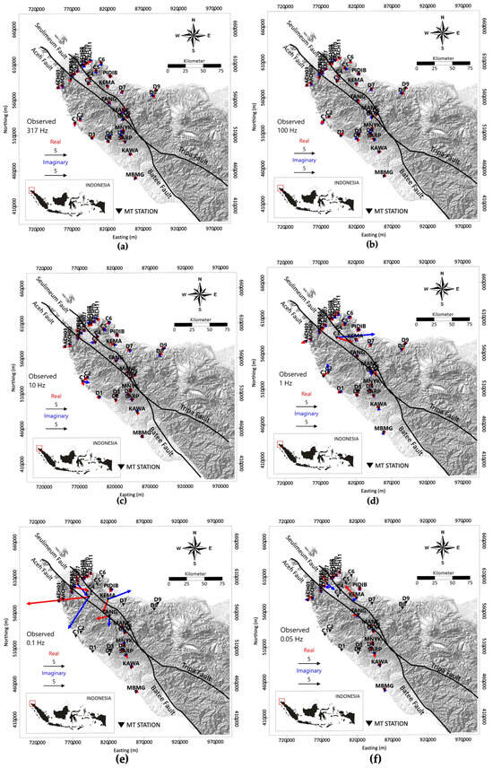
Figure 8.
Induction arrows for frequencies of (a) 317 Hz, (b) 100 Hz, (c) 10 Hz, (d) 1 Hz, (e) 0.1 Hz, and (f) 0.05 Hz in the same scale of induction arrows. The red arrows depict the real part of tipper vector and the black diagrams depict the imaginery part of tipper vector (using Parkinson convention, red arrows point to the conducting body).
4.3. Groom–Bailey Decomposition and the Depth of Penetration (DOP)
In addition to using dimensional analysis, such as polar diagrams and induction arrows, the MT data were also analyzed using the Groom–Bailey decomposition technique to identify regional conductivity strikes. The Groom–Bailey decomposition technique at each MT station (Figure 9) helps verify the presence of geological strikes for fault analysis. The Groom–Bailey decomposition technique applied in the MT data is plotted in the rose diagrams of the regional conductivity strikes. Those diagrams were calculated for each station at multiple frequencies before calculating the average value of them as shown in Figure 9. The average value showed the direction of the conductivity strike in the study area, which was shown to be relatively northwest (NW)–southeast (SE) with an angle of S 71.61° E, which was also confirmed by geological study [7]. The result of the Groom–Bailey decomposition in Figure 9 confirms the induction arrows analysis in Figure 7.
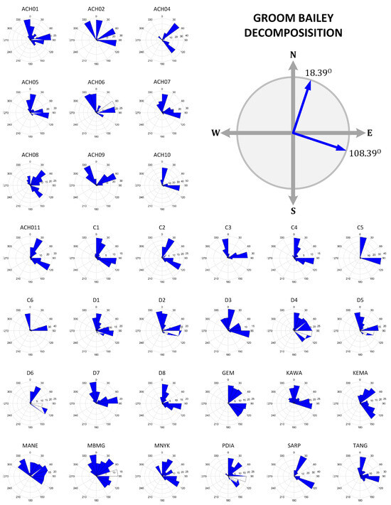
Figure 9.
Regional conductivity strike direction of the Sumatran Fault System area based on the Groom–Bailey decomposition technique.
Data resolution analysis was performed based on the depth of penetration (DOP), which is mathematically given by Equation (21) [60]:
The data resolution analysis using DOP compared to the model resulted from inversion, which was used qualitatively to validate the depth sensitivity of the model. The DOP plot was analyzed at several frequencies as given in Figure 10: 320 Hz, 100 Hz, 10 Hz, 1 Hz, 0.1 Hz, and 0.05 Hz. The representative frequencies with specifically high frequency at 10 Hz and low frequency at 0.1 Hz have been reported below. The DOP for the high frequency (f = 320 Hz) has a range of approximately 0.02 km to 0.37 km in Figure 10a. The depth of 0.02 km corresponds to the low-resistivity zones in the eastern of the Aceh Segment, as shown in the pseudosection in Figure 11a, while the depth of 0.37 km corresponds to the high-resistivity zones in the western of the Aceh Segment, as shown in the pseudosection in Figure 11a. This is consistent with the skin depth concept, where the low-resistivity zones have shallower field penetration depth, while the high-resistivity zones have deeper field penetration depth. Next, the DOP for the low frequency (f = 0.1 Hz) ranges from approximately 2.24 km to 57.49 km, as shown in Figure 10e. The depth of 2.24 km corresponds to the low-resistivity zones in the eastern of the Aceh segment, as shown in the pseudosection in Figure 11e, while the depth of 57.49 km corresponds to the high-resistivity zones in the west of the Aceh segment, as given in Figure 11e. This is also consistent with the skin depth concept, where the low-resistivity zones have shallower field penetration depth, while the high-resistivity zones have a deeper field penetration depth. Figure 10b shows the depth of penetration at a high frequency of 100 Hz, with a range of approximately 0.04 km to 0.89 km. Figure 10c shows the depth of penetration at a high frequency of 10 Hz, with a range of approximately 0.19 km to 2.97 km. Figure 10d shows the depth of penetration at a high frequency of 1 Hz, with a range of approximately 0.44 km to 10.07 km. Figure 10e shows the depth of penetration at a high frequency of 0.1 Hz, with a range of approximately 2.24 km to 57.49 km. Figure 10f shows the depth of penetration at a high frequency of 0.05 Hz, with a range of approximately 3.32 km to 71.11 km. These values correspond to the pseudosection in Figure 11b–f, which matches the skin depth concept. The other frequencies (f = 320 Hz, f = 100 Hz, f = 1 Hz, and f = 0.05 Hz) show the same pattern, with frequencies of 10 Hz and 0.1 Hz where the DOP of the low-resistivity zone corresponds to the shallower depth and the DOP of the high-resistivity zone corresponds to the deeper depth of the pseudosection, as shown in Figure 11.
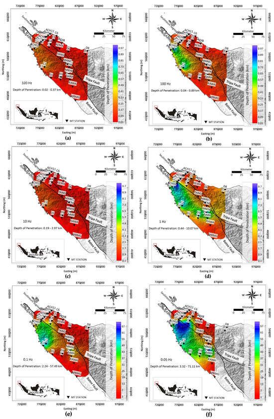
Figure 10.
Depth of penetration at frequencies of (a) 320 Hz, (b) 100 Hz, (c) 10 Hz, (d) 1 Hz, (e) 0.1 Hz, and (f) 0.05 Hz.
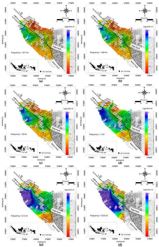
Figure 11.
Planar view the pseudosection of MT data at frequencies of (a) 320 Hz, (b) 100 Hz, (c) 10 Hz, (d) 1 Hz, (e) 0.1 Hz and (f) 0.05 Hz.
4.4. Three-Dimensional Inversion Model of MT Data
We present our preferred 3D model of the electrical structure of the northern Sumatran Fault zones, based on full inversion of impedances as given in Figure 12a with the RMS error given in Figure 12b. The horizontal cross-sections at several interval depths from ~0 km to ~5 km are given in Figure 13 to better show the continuity of the resistivity zone. The horizontal cross-sections resulting from the inversion in Figure 13 are confirmed by the DOP analysis in Figure 10 by qualitative comparison of the pseudosection, which has a depth that includes the depth of the horizontal cross-section. The pseudosection of the DOP at a frequency of 10 Hz ranging from 0.19 km to 2.97 km is given in Figure 11c, and it has been compared qualitatively to the horizontal cross-section at the depth of 1 km, as shown in Figure 13b. It can be seen that the east of the Aceh Segment is dominated by low-resistivity zones, as shown in Figure 13b, which qualitatively match the low-resistivity zones of the pseudosection in the east of the Aceh Segment at a frequency of 10 Hz, as shown in Figure 11c. Similarly, the high-resistivity zones in the west of the Aceh Segment shown in Figure 13b match with the high-resistivity zones of the pseudosection in the western of the Aceh Segment at frequency of 10 Hz, as shown in Figure 11c. Furthermore, the horizontal cross-sections at the other depths (depth of 2 km, 3 km, 4 km, and 5 km) were also analyzed using DOP analysis, in the same way as previously performed. It can therefore be assumed that the anomalies calculated by the model can be reliably interpreted. This assumption is supported by the RMS error given in Figure 12b, which has a downtrend pattern. The RMS of the last iteration of this inversion is 7.138.
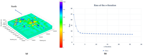
Figure 12.
(a) A 3D view of the resistivity distribution model beneath the Aceh Segment and Seulimeum Segment of the Sumatran Fault Zone and (b) the RMS error of the inversion result. The black triangles depict the MT station.
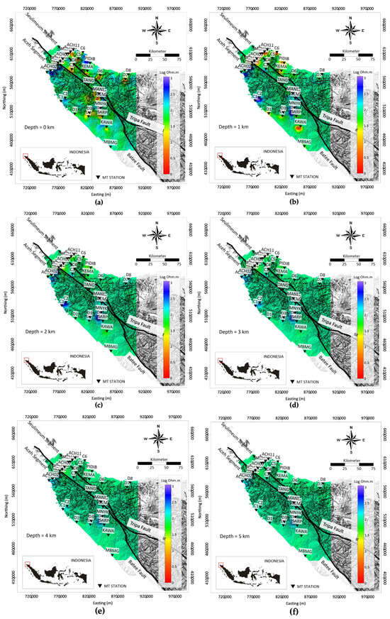
Figure 13.
The horizontal cross-section of the 3D resistivity model from (a) 0 km, (b) 1 km, (c) 2 km, (d) 3 km, (e) 4 km, and (f) 5 km beneath the Earth’s surface.
To see an overview of the RMS conditions that reached 7.138 in the model, an analysis was carried out by taking several samples of the observed data and the calculated data from several stations (six stations), as shown in Figure 14. The observed and calculated data of those samples were compared to each other, including the apparent resistivity and phase curves. The apparent resistivity and phase curves between the observed and calculated data from six stations had to fit each other for both yx-data components and xy-data components, which showed the same pattern. It can be concluded that the data calculated from the inversion represent the observed data from the field measurements. For further studies of the resistivity cross-section of the 3D Earth model and to characterize the Aceh Segment and Seulimeum segment faults, the inversion result was investigated in three profiles in Figure 15: Profile 1 (P1), Profile 2 (P2), and Profile 3 (P3). Those profiles were selected to show the representative images that cut across the fault direction (P1 and P2 are perpendicular to the fault direction, while P3 forms a certain angle to the fault direction). The cross-sections of P1, P2, and P3 are given in Figure 16, Figure 17, and Figure 18, respectively.
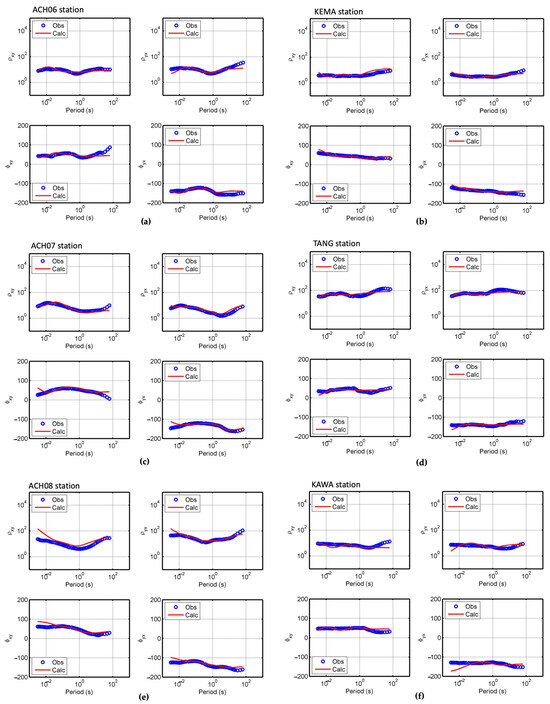
Figure 14.
Apparent resistivity and phase between observed and calculated data from 3D inversion of MT data from the (a) ACH06 (b) KEMA, (c) ACH07, (d) TANG, (e) ACH08, and (f) KAWA stations.
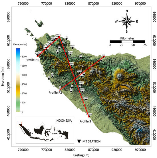
Figure 15.
Profile map for further studies of the resistivity cross-section (noted by the red straight line with the label).
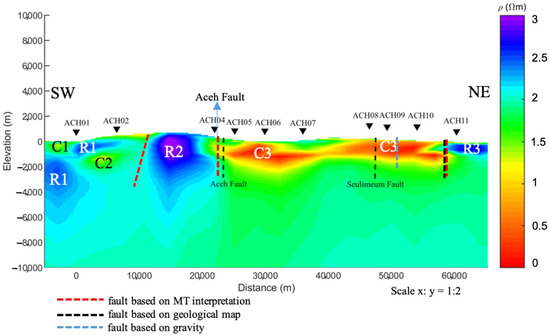
Figure 16.
Profile 1 (P1) of the 3D resistivity model.
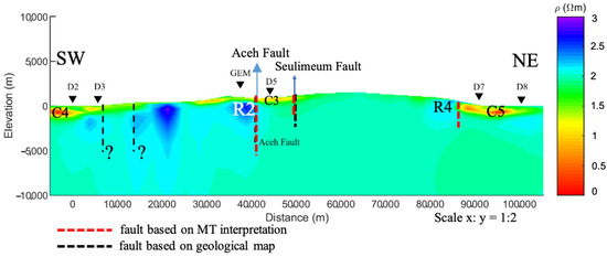
Figure 17.
Profile 2 (P2) of the 3D resistivity model. The black question mark symbols (?) depict the unknown faults.
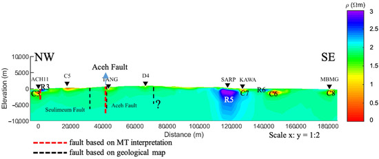
Figure 18.
Profile 3 (P3) of the 3D resistivity model. The black question mark symbol (?) depicts the unknown fault.
5. Discussion
Interpretation of cross-section P1 was performed by comparing this section with the Banda Aceh geological map, as shown in Figure 1, starting from station ACH01 and going through to ACH11 sequentially. This method identified that the low-resistivity area C1 consists of sedimentary and metasedimentary rocks (marine/continental sediment) in the form of alluvium, with resistivity values ranging from 10 to 800 Ωm [61], corresponding to the resistivity depicted in the MT cross-section of P1. The high-resistivity area R1 was identified as igneous rock, consisting of limestone formations with a resistivity range of 2 × 10⁴ to 2 × 10⁶ Ωm [62], from the Lamno Formation, limestone from the Raba Formation, and metamorphic rocks consisting of agglomerates (Quartz rocks) from the Bentaro Volcanic Formation, which matches with the depicted resistivity in the MT cross-section of P1. According to the geological map in Figure 1, Miocene and Quaternary volcanic rocks and sedimentary rocks were identified in Figure 16 as C2. The resistivity contrast between R1, C1, and C2 is not identified as a fault because, based on the references, this area records low seismic activity [25].
Then, between stations ACH04 and ACH05, based on the MT cross-section of P1 in Figure 15, there is a resistivity contrast from a distance of 20–30 km, as shown in the MT cross-section of P1 in Figure 15, which is interpreted as the Aceh Segment, a part of the Sumatran Fault, and confirmed by the geological map in Figure 1; this is further supported by gravity anomaly analysis references [25]. This analysis indicates a difference in vertical block densities, with high densities (2.4–2.55 g/cm3) and low densities (2.2–2.4 g/cm3) over a distance of 25–50 km, which aligns with the MT cross-section results at a distance of 20–30 km and a dip angle of 90°, as per reference [25].
Based on the MT section in Figure 16, a creep zone (C3) characterized by a conductive zone is visible at a depth of 2 km, confirmed by the existence of the creeping zone in the Aceh Segment along ~100 km [55]. Characterizing the creeping zone corresponds to the presence of the fluids related to the old terrace deposits of the Indrapuri Formation characteristics. The Indrapuri Formation is characterized by volcanic rocks, including tuffaceous and calcareous sandstones, which can contain fluids such as water and contribute to low-resistivity zones.
The high-resistivity zone with a range of 150–1000 Ωm (R2) is characterized as basement rock, specifically metamorphic rocks from the Triassic–Cretaceous age, as confirmed by the geological map in Figure 1. The low-resistivity zone with resistivity values of 1–15 Ωm (C3) is characterized as volcanic rock from the Lam Teuba Volcanic Formation and the Indrapuri Formation, consisting of old terrace deposits and volcanic gravels, which tend to have low resistivity [63], as confirmed by the geological map in Figure 1, consistent with the MT cross-section in Figure 16. Further, between 55 and 60 km, the Seulimeum Fault Segment is not visible on the MT cross-section of P1. Nevertheless, the Seulimeum Fault Segment can be confirmed by gravity anomaly, indicating a difference in rock densities [25], and the geological map in Figure 1. The northeastern of P1 is identified as an unknown fault from the MT cross-section of P1 in Figure 16, which confirms the minor fault in the geological map in Figure 1, where the low-resistivity zone is quaternary volcanic rocks with a resistivity of 1–15 Ωm (C3) and the high-resistivity zone (R3) comprises andesite rocks (4.5 × 10⁴–1.7 × 10⁵ m) that do not continue downwards, as depicted by Figure 16.
Based on the MT cross-section of P2 in Figure 17, the Aceh Segment Fault is still visible at a distance of 40–50 km, marked by a resistivity contrast similar to the P1 cross-section. Meanwhile, based on the MT cross-section of P2, the Seulimeum Segment Fault is visible between a distance of 55–60 km compared to P1, which is invisible. It is found in the MT cross-section of P2 that beneath station D2 in the southwest (SW), there is an alluvium rock formation indicated by a low-resistivity zone (C4) in the range of 1–20 Ωm, which corresponds with the geological map in Figure 1. Furthermore, at distances between 10–20 km and 80–90 km, there is a known resistivity contrast indicated as small faults, which confirms the minor unknown fault in the geological map. Meanwhile, beneath station D7, there is a low-resistivity zone (C5) interpreted to be sandstone from the Peutu Formation, and the resistivity matches the MT cross-section. The high-resistivity zone (R4) is interpreted as basement igneous rock consisting of limestone, with resistivity matching the MT cross-section of P2 in Figure 17.
Based on the MT cross-section of P3 shown in Figure 18, it is found that the Aceh Segment Fault distance of 40–50 km does not show a resistivity contrast in the MT cross-section as is seen in P1 and P2. The Seulimeum Segment Fault is also not detected as having resistivity contrast in this MT cross-section of P3. However, further information can be interpreted from the MT cross-section of P3. This information indicates that beneath the ACH11 station, andesite rock (4.5 × 10⁴–1.7 × 10⁵ m) is visible in the high-resistivity zone (R3), while the low-resistivity zone (C3) is characterized as quaternary volcanic rock with a resistivity of 1–15 Ωm, which is the same as that shown in the MT cross-section of P1. Then, beneath the SARP station, a high-resistivity zone (R5) is interpreted as basement rock in metamorphic rock, corresponding with the geological map in Figure 1, as its depth reaches 10 km, as shown in Figure 18. Meanwhile, the low-resistivity zone (C7) beneath KAWA station is interpreted as an alluvial sediment layer with a resistivity of 5–10 Ωm, matching the MT cross-section of P3 in Figure 18, where the conductive layer does not continue downward. Next, the high-resistivity zone (R6) is the Tutut Formation, which is resistive with a resistivity range of 100–500 Ωm [64]. The low-resistivity zone (C6) is the Meulaboh Formation, consisting of semi-consolidated sands and gravels with a resistivity range of 30–225 Ωm [65]. Finally, at the southwestern-most end (SW) of P3 shown in Figure 18 is station MBMG, which indicates the presence of conductive material interpreted as alluvial sediment rock with a resistivity range of 5–10 Ωm. It can be concluded that these interpretations of the MT cross-section of P3 are aligned with the geological map in Figure 1.
6. Conclusions
The Sumatran Fault system was confirmed from MT data as A strike-slip fault where the average value of the direction of the conductivity strike was shown to be relatively northwest (NW)–southeast (SE), with an angle of S 71.61° E. In the northern part of the Sumatran Fault system, the fault bifurcates into the Aceh and Seulimeum segments. Based on the MT cross-section resulting from the 33 MT stations, we could obtain information about the Aceh Fault Segment’s location, which is 20–30 km, with the creeping zone found at 2 km. Meanwhile, the location of the Seulimeum Fault Segment is 55–60 km. The results agree well with the geological map and the anomaly gravity around them. Furthermore, we can confirm many formations beneath the Sumatran Fault System, especially near the Aceh Fault Segment and Seulimeum Fault Segment. It can also be concluded that the western part of the Aceh Fault Segment dominated by the basement rock, specifically metamorphic rocks from the Triassic–Cretaceous age, is characterized by a high-resistivity zone, with a resistivity range of 150–1000 Ωm. The zone between the Aceh Fault Segment and the Seulimeum Fault Segment is found to be a low-resistivity zone with resistivity values of 1–15 Ωm, characterized as volcanic rocks from the Lam Teuba Volcanic Formation and the Indrapuri Formation, consisting of old terrace deposits and volcanic gravels. Further, the eastern part of the Seulimeum Fault Segment is dominated with low resistivity, with a resistivity of 1–15 Ωm, characterized as quaternary volcanic rock, and a high-resistivity zone, which is characterized as andesite rock (4.5 × 10⁴–1.7 × 10⁵ m) that does not continue downwards. The results of the MT cross-section confirm the geological map.
Author Contributions
Data curation: L.Y.R., N., T. and P.M.P.; Funding acquisition: Y.O.; Investigation: Y.O. and D.S. (Didik Sugiyanto); Resources: P.M.P. and W.S.; Supervision: N., D.S. (Doddy Sutarno) and W.S.; Visualization: L.Y.R., T., A.S. and P.M.P.; Writing—original draft: L.Y.R.; Writing—review and editing: N. and S. All authors have read and agreed to the published version of the manuscript.
Funding
This research received no external funding.
Institutional Review Board Statement
Not applicable.
Informed Consent Statement
Not applicable.
Data Availability Statement
The raw data supporting the conclusions of this article will be made available by the authors on request.
Acknowledgments
The authors would like to thank the Laboratory of Modelling and Inversion, Physics of Earth and Complex Systems, ITB, for the permission to use its facilities in support of this study.
Conflicts of Interest
All authors declare that the research was conducted in the absence of any commercial or financial relationship that could be construed as a potential conflict of interest.
References
- DeMets, C.; Gordon, R.G.; Argus, D.F. Geologically Current Plate Motions. Geophys. J. Int. 2010, 181, 1–80. [Google Scholar] [CrossRef]
- Fitch, T.J. Plate Convergence, Transcurrent Faults, and Internal Deformation Adjacent to Southeast Asia and the Western Pacific. J. Geophys. Res. 1972, 77, 4432–4460. [Google Scholar] [CrossRef]
- Hamilton, W. Tectonics of the Indonesian Region; U.S. Government Publishing Office: Washington, DC, USA, 1979.
- Genrich, J.F.; Bock, Y.; McCaffrey, R.; Prawirodirdjo, L.; Stevens, C.W.; Puntodewo, S.S.O.; Subarya, C.; Wdowinski, S. Distribution of Slip at the Northern Sumatran Fault System. J. Geophys. Res. Solid Earth 2000, 105, 28327–28341. [Google Scholar] [CrossRef]
- Curray, J.R. Tectonics and History of the Andaman Sea Region. J. Asian Earth Sci. 2005, 25, 187–232. [Google Scholar] [CrossRef]
- Fernández-Blanco, D.; Philippon, M.; von Hagke, C. Structure and Kinematics of the Sumatran Fault System in North Sumatra (Indonesia). Tectonophysics 2016, 693, 453–464. [Google Scholar] [CrossRef][Green Version]
- Sieh, K.; Natawidjaja, D. Neotectonics of the Sumatran Fault, Indonesia. J. Geophys. Res. Solid Earth 2000, 105, 28295–28326. [Google Scholar] [CrossRef]
- Febriansyah Putra, A.; Chenrai, P. Geomorphic Interpretation on the Formation of Strike-Slip Basins along the Northern Sumatran Fault. J. Asian Earth Sci. X 2023, 10, 100167. [Google Scholar] [CrossRef]
- Ito, T.; Gunawan, E.; Kimata, F.; Tabei, T.; Simons, M.; Meilano, I.; Agustan; Ohta, Y.; Nurdin, I.; Sugiyanto, D. Isolating Along-strike Variations in the Depth Extent of Shallow Creep and Fault Locking on the Northern Great Sumatran Fault. J. Geophys. Res. Solid Earth 2012, 117, B06409. [Google Scholar] [CrossRef]
- Natawidjaja, D.; Sieh, K. Slip Rate along the Sumatran Transcurrent Fault and Its Tectonic Significance. In Proceedings of the Conference on Tectonic Evolution of Southeast Asia, London, UK, 21–24 August 1994; Volume 7–8. [Google Scholar]
- Sieh, K.; Zachariasen, J.; Bock, Y.; Edwards, L.; Taylor, F.; Gans, P. Active Tectonics of Sumatra. Geol. Soc. Am. Abstr. Programs 1994, 26, 382. [Google Scholar]
- Bellier, O.; Sébrier, M. Is the Slip Rate Variation on the Great Sumatran Fault Accommodated by Fore-arc Stretching? Geophys. Res. Lett. 1995, 22, 1969–1972. [Google Scholar] [CrossRef]
- Bennet, J.D.; Brige, D.M.C.; Cameron, N.R.; Djunuddin, A.; Ghazali, S.A.; Jeffery, D.H.; Kartawa, W.; Keats, W.; Rock, N.M.S.; Thosmson, S.J.; et al. Geological Map of Banda Aceh Sheet, Scale 1: 250.000; Indonesian Geological Research and Development Center: Bandung, Indonesia, 1981. [Google Scholar]
- Hurukawa, N.; Wulandari, B.R.; Kasahara, M. Earthquake History of the Sumatran Fault, Indonesia, since 1892, Derived from Relocation of Large Earthquakes. Bull. Seismol. Soc. Am. 2014, 104, 1750–1762. [Google Scholar] [CrossRef]
- Cagniard, L. Basic theory of the magneto-telluric method of geophysical prospecting. Geophysics 1953, 18, 605–635. [Google Scholar] [CrossRef]
- Tikhonov, A.N. On Determining Electrical Characteristics of the Deep Layers of the Earth’s Crust. Doklady 1950, 73, 295–297. [Google Scholar]
- Simpson, F.; Bahr, K. Practical Magnetotellurics; Cambridge University Press: Cambridge, UK, 2005. [Google Scholar]
- Berdichevsky, M.; Dmitriev, V. Models and Methods of Magnetotellurics; Springer: Berlin/Heidelberg, Germany, 2008. [Google Scholar]
- Zhang, L.; Unsworth, M.; Jin, S.; Wei, W.; Ye, G.; Jones, A.G.; Jing, J.; Dong, H.; Xie, C.; Le Pape, F.; et al. Structure of the Central Altyn Tagh Fault Revealed by Magnetotelluric Data: New Insights into the Structure of the Northern Margin of the India–Asia Collision. Earth Planet. Sci. Lett. 2015, 415, 67–79. [Google Scholar] [CrossRef]
- Oryński, S.; Jóźwiak, W.; Nowożyński, K. An Integrative 3-D Model of the Deep Lithospheric Structure beneath Dolsk and Odra Fault Zones as a Result of Magnetotelluric Data Interpretation. Geophys. J. Int. 2021, 227, 1917–1936. [Google Scholar] [CrossRef]
- He, M.; Xu, Y.; Fang, H.; Zhang, X. Deep Structure and Formation Model of the Southernmost Tanlu Fault Zone, Eastern China: Constrained from Magnetotelluric Imaging. J. Asian Earth Sci. 2023, 256, 105805. [Google Scholar] [CrossRef]
- Nurhasan; Ogawa, Y.; Kimata, F.; Sutarno, D.; Sugiyanto, D.; Ismail, N. Identification of Sumatran Fault Zone Using Magnetotelluric and Garvity Data. In Proceedings of the 13th SEGJ International Symposium, Tokyo, Japan, 12–14 November 2018; Society of Exploration Geophysicists and Society of Exploration Geophysicists of Japan: Tokyo, Japan, 2019; pp. 182–185. [Google Scholar]
- Ogawa, Y.; Uchida, T. A Two-Dimensional Magnetotelluric Inversion Assuming Gaussian Static Shift. Geophys. J. Int. 1996, 126, 69–76. [Google Scholar] [CrossRef]
- Sutarno, D.; Ogawa, Y.; Prihantoro, R.; Sugiyanto, D.; Ismail, N.; Kimata, F. Electrical Resistivity Imaging of Sumatran Fault Based on Magnetotelluric Data. In Proceedings of the 22nd EM Induction Workshop, Weimar, Germany, 24–30 August 2014. [Google Scholar]
- Yanis, M.; Abdullah, F.; Zaini, N.; Ismail, N. The Northernmost Part of the Great Sumatran Fault Map and Images Derived from Gravity Anomaly. Acta Geophys. 2021, 69, 795–807. [Google Scholar] [CrossRef]
- Syukri, M.; Saad, R. Seulimeum Segment Characteristic Indicated by 2-D Resistivity Imaging Method. NRIAG J. Astron. Geophys. 2017, 6, 210–217. [Google Scholar] [CrossRef][Green Version]
- Natawidjaja, D.H. Neotectonics of the Sumatran Fault and Paleogeodesy of the Sumatran Subduction Zone; California Institute of Technology: Pasadena, CA, USA, 2003. [Google Scholar]
- Barber, A.; Crow, M.; Milsom, J. Introduction and Previous Research. In Sumatra: Geology, Resources and Tectonic Evolution; Geological Society of London: London, UK, 2005. [Google Scholar]
- Singh, S.C.; Moeremans, R.; McArdle, J.; Johansen, K. Seismic Images of the Sliver Strike-slip Fault and Back Thrust in the Andaman-Nicobar Region. J. Geophys. Res. Solid. Earth 2013, 118, 5208–5224. [Google Scholar] [CrossRef]
- Fontaine, H.; Gafoer, S. The Pre-Tertiary Fossils of Sumatra and Their Environments; CCOP Technical Secretariat: Bangkok, Thailand, 1989. [Google Scholar]
- Cameron, N.R.; Bennett, J.D.; Bridge, D.M.; Clarke, M.C.G.; Djunuddin, A.; Ghazali, S.A.; Harahap, H.; Jeffery, D.H.; Kartawa, W.; Keats, W.; et al. Geological Map of Takengon Sheet, Sumatra, Scale 1: 250.000; Indonesian Geological Research and Development Center: Bandung, Indonesia, 1983. [Google Scholar]
- Hady, A.K.; Marliyani, G.I. Updated Segmentation Model of the Aceh Segment of the Great Sumatran Fault System in Northern Sumatra, Indonesia. J. Appl. Geol. 2020, 5, 84–100. [Google Scholar] [CrossRef]
- Natawidjaja, D.H.; Triyoso, W. The Sumatran Fault Zone—From Source to Hazard. J. Earthq. Tsunami 2007, 1, 21–47. [Google Scholar] [CrossRef]
- Curray, J.R.; Moore, D.G.; Lawver, L.A.; Emmel, F.J.; Raitt, R.W.; Henry, M.; Kieckhefer, R. Tectonics of Andaman Sea and Burma, in Geological and Geophysical Investigations of Continental Margins. Amer. Assoc. Petrol. Geol. Mem. 1979, 29, 189–198. [Google Scholar]
- Moechtar, H.; Subiyanto, S.; Sugianto, D. Geologi Aluvium Dan Karakter Endapan Pantai/Pematang Pantai di Lembah Krueng Aceh, Aceh Besar (Prov. NAD). J. Geol. Dan. Sumberd. Miner. 2009, 19, 273–283. [Google Scholar] [CrossRef]
- Kumar, S. Tipper Magnitude: A Possible Indicator of Anomalous Conducting Zone. J. Geophys. 2017, XXXV, 83–87. [Google Scholar]
- Muksin, U.; Irwandi; Rusydy, I.; Muzli; Erbas, K.; Marwan; Asrillah; Muzakir; Ismail, N. Investigation of Aceh Segment and Seulimeum Fault by Using Seismological Data; A Preliminary Result. J. Phys. Conf. Ser. 2018, 1011, 012031. [Google Scholar] [CrossRef]
- Wait, J.R. Theory of Magnetotelluric Fields. J. Res. NBS D 1962, 66, 509–541. [Google Scholar] [CrossRef]
- Berdichevsky, M.N.; Dmitriev, V.I. Magnetotellurics in the Context of the Theory of Ill-Posed Problems; Society of Exploration Geophysicists: Tulsa, OK, USA, 2002. [Google Scholar]
- Sutarno, D.; Vozoff, K. Robust M-Estimation of Magnetotelluric Impedance Tensors. Explor. Geophys. 1989, 20, 383–398. [Google Scholar] [CrossRef]
- Egbert, G.D.; Booker, J.R. Robust Estimation of Geomagnetic Transfer Functions. Geophys. J. Int. 1986, 87, 173–194. [Google Scholar] [CrossRef]
- Zorin, N.; Aleksanova, E.; Shimizu, H.; Yakovlev, D. Validity of the Dispersion Relations in Magnetotellurics: Part I—Theory. Earth Planets Space 2020, 72, 9. [Google Scholar] [CrossRef]
- Weidelt, P. The Inverse Problem of Geomagnetic Induction. Z. Geophys. 1972, 38, 257–289. [Google Scholar] [CrossRef][Green Version]
- Caldwell, T.G.; Bibby, H.M.; Brown, C. The Magnetotelluric Phase Tensor. Geophys. J. Int. 2004, 158, 457–469. [Google Scholar] [CrossRef]
- Berdichevsky, M.N.; Vanyan, L.L.; Koshurnikov, A.V. The Baikal Rift Zone: Magnetotelluric Arbitration of Geodynamic Models. In Proceedings of the XIV Workshop on EM induction in the Earth, Sinaia, Romania, 16–22 August 1998. [Google Scholar]
- Berdichevsky, M.N.; Vanyan, L.L.; Nguen, T.V. Phase Polar Diagrams of the Magnetotelluric Impedance. Izv. Akad. Nauk. SSSR Ser. Fiz. Zemli 1993, 2, 19–23. [Google Scholar]
- Berdichevsky, M.N. Electrical Prospecting by the Method of Magnetotelluric Profiling: Moscow; Nedra Publishing House: Moscow, Russia, 1968. [Google Scholar]
- Chave, A.D.; Jone, A.G. The Magnetotelluric Method: Theory and Practice; Cambridge University Press: New York, NY, USA, 2012. [Google Scholar]
- Parkinson, W.D. The Influence of Continents and Oceans on Geomagnetic Variations. Geophys. J. R. Astron. Soc. 1962, 6, 441–449. [Google Scholar] [CrossRef]
- Wiese, H. Geomagnetishce Tiefentellurik. Geofis. Pura Appl. 1962, 52, 83–103. [Google Scholar] [CrossRef]
- Kelbert, A.; Meqbel, N.; Egbert, G.D.; Tandon, K. ModEM: A Modular System for Inversion of Electromagnetic Geophysical Data. Comput. Geosci. 2014, 66, 40–53. [Google Scholar] [CrossRef]
- Egbert, G.D.; Kelbert, A. Computational recipes for electromagnetic inverse problems. Geophys. J. Int. 2012, 189, 251–267. [Google Scholar] [CrossRef]
- Evans, R.L.; Chave, A.D.; Jones, A.G.; Mackie, R.; Rodi, W. Conductivity of Earth Materials. In The Magnetotelluric Method: Theory and Practice; Chave, A.D., Jones, A.G., Eds.; Cambridge University Press: Cambridge, UK, 2012; ISBN 9781139020138. [Google Scholar]
- Selway, K. Electrical Discontinuities in the Continental Lithosphere Imaged with Magnetotellurics; AGU Publications: Washington, DC, USA, 2018; pp. 89–109. [Google Scholar]
- Glover, P.W.J. Geophysical Properties of the Near Surface Earth: Electrical Properties. In Treatise on Geophysics; Elsevier: Amsterdam, The Netherlands, 2015; pp. 89–137. [Google Scholar]
- Slezak, K.; Jozwiak, W.; Nowozynski, K.; Orynski, S.; Brasse, H. 3-D Studies of MT Data in the Central Polish Basin: Influence of Inversion Parameters, Model Space and Transfer Function Selection. J. Appl. Geophys. 2019, 161, 26–36. [Google Scholar] [CrossRef]
- Siripunvaraporn, W.; Egbert, G.; Uyeshima, M. WSINV3DMT Version 1.0.0 for Single Processor Machine. pp. 1–21. Available online: https://manualzz.com/doc/6812773/wsinv3dmt-magnetotelluric-inversion-user-manual (accessed on 5 August 2020).
- Hady, A.K.; Marliyani, G.I. Updated Segmentation Model and Cummulative Offset Measurement of the Aceh Segment of the Sumatran Fault System in West Sumatra, Indonesia. J. Appl. Geol. 2021, 5, 84. [Google Scholar] [CrossRef]
- Hoffmann-Rothe, A.; Ritter, O.; Haak, V. Magnetotelluric and Geomagnetic Modelling Reveals Zones of Very High Electrical Conductivity in the Upper Crust of Central Java. Phys. Earth Planet. Inter. 2001, 124, 131–151. [Google Scholar] [CrossRef]
- d’Erceville, I.; Kunetz, G. The effect of a fault on the earth’s natural electromagnetic field. Geophysics 1962, 27, 651–665. [Google Scholar] [CrossRef]
- Halliday, D.; Resnick, R.; Walker, J. Fundamentals of Physics, 6th ed.; John Wiley & Sons, Inc.: Hoboken, NJ, USA, 1991. [Google Scholar]
- Telford, W.M.; Geldart, L.P.; Sheriff, R.E. Applied Geophysics; Cambridge University Press: Cambridge, UK, 1976. [Google Scholar]
- Ghorbani, A.; Revil, A.; Coperey, A.; Soueid Ahmed, A.; Roque, S.; Heap, M.J.; Grandis, H.; Viveiros, F. Complex Conductivity of Volcanic Rocks and the Geophysical Mapping of Alteration in Volcanoes. J. Volcanol. Geotherm. Res. 2018, 357, 106–127. [Google Scholar] [CrossRef]
- Rahmadi, R.; Setiawan, B.; Aziz, M. Analisis Karakteristik Endapan Emas Plaser di Daerah Kecamatan Sungai Mas dan Sekitarnya, Kabupaten Aceh Barat, Provinsi Aceh. Acta Geosci. Energy Min. 2023, 2, 32–38. [Google Scholar]
- Park, C.-S.; Jeong, J.-H.; Park, H.-W.; Kim, K. Experimental Study on Electrode Method for Electrical Resistivity Survey to Detect Cavities under Road Pavements. Sustainability 2017, 9, 2320. [Google Scholar] [CrossRef]
Disclaimer/Publisher’s Note: The statements, opinions and data contained in all publications are solely those of the individual author(s) and contributor(s) and not of MDPI and/or the editor(s). MDPI and/or the editor(s) disclaim responsibility for any injury to people or property resulting from any ideas, methods, instructions or products referred to in the content. |
© 2024 by the authors. Licensee MDPI, Basel, Switzerland. This article is an open access article distributed under the terms and conditions of the Creative Commons Attribution (CC BY) license (https://creativecommons.org/licenses/by/4.0/).