Threading Statistical Disclosure Attack with EM: An Algorithm for Revealing Identity in Anonymous Communication Networks

Abstract

Messages sent across multiple platforms can be correlated to infer users’ attitudes, behaviors, preferences, lifestyles, and more. Therefore, research on anonymous communication systems has intensified in the last few years. This research introduces a new algorithm, Threading Statistical Disclosure Attack with EM (TSDA-EM), that employs real-world data to reveal communication’s behavior in an anonymous social network. In this study, we utilize a network constructed from email exchanges to represent interactions between individuals within an institution. The proposed algorithm is capable of identifying communication patterns within a mixed network, even under the observation of a global passive attacker. By employing multi-threading, this implementation reduced the average execution time by a factor of five when using a dataset with a large number of participants. Additionally, it has markedly improved classification accuracy, detecting more than 79% of users’ communications in large networks and more than 95% in small ones.

1. Introduction

The continuous use of the Internet for all kinds of human activities has resulted in an unprecedented proliferation of data across multiple platforms, which can be used to attack everybody’s privacy  [1]. As a result, experts and researchers have recommended employing privacy-preserving technologies to protect society from digital threats [2]. Moreover, it has been argued that privacy protection should not be optional but mandatory, even when there is a trade-off between security and liberty [3]. More worrisome is the fact that people’s information is currently stored in many databases, and if these can be correlated, the produced metadata may be exploited to measure individuals’ behaviors, preferences, attitudes, health, stress levels, demographics, sleep habits, exercising, etc. [4,5,6].

Personal data are any information referring to some identified or identifiable person. Collecting personal data about multiple people has tremendous value for data brokers, because they are usually avid to gather as much information as possible in order to sell it. It is already known that free services over the Internet have a hidden cost, since our metadata are exposed [7,8]. Personal data are considered an article of trade by technological platforms, which exchange it in return for a free service. It has been stated that young people surrender their personal information more easily to obtain a service, get more followers on social media, establish an attractive profile, and engage in other apparently naive activities [9].

Email networks, constructed by the exchange of messages between people, can be used as a proxy for the professional relationship between individuals in an organization. Therefore, other researchers have classified it as a social network [10,11,12] that can provide information about personal acquaintances, how groups of people work to complete a task, or how information flows across an organization. In other words, the exchange of emails may reveal private information about individuals and their workplace. It has been proved that traffic analysis can be used to infer personal data, even when privacy protection mechanisms are used in an anonymous communication channel [13]. Also, some of the authors in this paper have carried out previous research on the mechanisms and consequences of inferring information from the communication data produced by anonymous social networks [14].

This research focuses on developing an algorithm to infer information even when the communication channels are protected with a mix network [15]. A mix network is a mechanism used to hide end-to-end communication from third parties. This mechanism stores messages from multiple senders, shuffles them, and sends them to their destinations, with the objective of breaking the relationship between senders and receivers. The algorithm proposed here is called Threading Statistical Disclosure Attack using the Expectation-Maximization Algorithm (TSDA-EM), and it is an improvement over two previous statistical disclosure attack algorithms [16,17]: The one in [16], which will be referred to as the Original Algorithm (OA) in this paper, infers communication within an anonymous social network but does not include threading and does not infer the frequency of messages. This research compares the results from the OA against the proposed TSDA-EM algorithm. On the other hand, the algorithm introduced in [17], called the Base Algorithm (BA) in here, describes how to calculate feasible tables and, using likelihood values, determines who is communicating with whom in an anonymous social network.

This research has implemented threads to speed up the algorithms. In computer programming, a thread is a short set of instructions planned to be scheduled and executed independently of the parent process. For instance, a program can have a thread waiting for a concrete incident to happen or running a different task, allowing the main program to perform other tasks.

In summary, our main contributions in this work are as follows:

• Developed an iterative algorithm to enhance the classification rate.
• Decreased the total execution time by an average of five times when processing data with a large number of participants. This reduction enables faster attacks on mixed networks despite the increased number of participants.
• Significantly improved our results using the EM algorithm, detecting more than 79% of users’ communications in large networks and over 95% in smaller ones.
• Inferred the frequency of messages between users. Rather than simply indicating communication with a binary value where 1 represents communication and 0 represents no communication, we have proposed quantifying the number of messages sent.

The remainder of this paper is organized as follows: Section 2 discusses previous related works, while Section 3 describes the theoretical framework. Section 4 introduces the TSDA-EM algorithm, and Section 5 describes its performance using a real-data social network. Finally, Section 6 concludes the article and proposes future work.

2. Related Works

Anonymous communication between users is still an unsolved research topic. In order to send messages over the Internet, there must be a source IP address and a destination IP address. Encryption can be used to provide confidentiality over the content of a message, but it does not offer protection against traffic analysis attacks. Chaum [15] proposed mix networks as a mechanism to obtain anonymous communication.

Anonymous communication may allow high latency of messages or require low latency. Examples of the first one are message-based systems such as cyberpunk remailers, anon.penet.fi, and mixminion [18,19]. These systems do not require an immediate response, like email systems. On the other hand, low-latency anonymous systems are based on onion routing like TOR [20], as they need real-time response; web applications, instant messenger, and secure shells belong to this category. For instance, Loopix, which is a mix network architecture centered around exponential mixes that use cover traffic to prevent traffic analysis attacks, as well as Vuvuzela design [21,22].

Anonymous communication networks aim to provide sender-unlinkability as well as other metrics of interest like unobservability, linkability, and undetectability. Most of these metrics are detailed in [23]. To guarantee sender unobservability, dummy traffic is often used. However, this overloads the communication channels, reduces throughput, and underutilizes bandwidth.

Agrawal and Kesdogan [24] proposed in 2003 to employ disjoint sets across communication observations to determine the exchange of information between users. The authors called this technique a disclosure attack. Danezis [25] built on this research by selecting a single user, Alice, and taking larger communication samples to determine the probability that other users exchange information with the first one. The authors termed this procedure a statistical disclosure attack (SDA).

From here on, there are many other studies that employ SDA to help determine the exchange of information between Alice and other users. In [26] the authors define the number of messages, n, that Alice might send with a probability $P_m\left(n\right)$, while [27] assumes that all users have n friends and they send messages with uniform probability. In [28], the authors introduce the hitting set attack (HSA), which focuses on finding the number of rounds needed to determine who is sending information to Alice with a set probability. Troncoso et al. [29] use a more general user behavior model, which they call Perfect Matching SDA (PMDA), where the number of the user’s friends and the distribution of sending probabilities toward them are not restricted. However, this study still uses synthetic data as input for its experiments. In a subsequent paper, Troncoso and Danezis [30] introduce BT-SDA, which employed Bayesian techniques and graph theory to infer the probability of paired communication; although they assume each user has a different number of friends, the probability of sending information is the same between them.

Later, the Reverse SDA (RSDA) algorithm [31] assumes that each message receives a response and uses this reverse observation to help determine the communication between users. Finally, Perez-Gonzales and Troncoso [32] employ least squares SDA (LSDA) to study the accuracy with which an adversary can identify the sender/receiver profile of Alice. Besides seeking to identify Alice’s message receivers, they also try to estimate the probability that Alice sends a message to them.

In [26], the authors introduce background noise, which initially should increase the difficulty to determine communication patterns between users. However, they also control users activity, which in the end helps them to obtain better predictions. In [27] the authors also include background noise to increase the difficulty of finding sending and receiving pairs; however, their data and assumptions are still far away from real scenarios. Emamdoost et. al. [33] improve on the use of noise by introducing cloak users that generate messages at the same time as Alice to increase the difficulty of finding communication patterns. Finally, other authors introduced Noise SDA (NSDA) [34], which analyzes the frequency of message co-occurrence between a target user and other users, allowing for more effective filtering of irrelevant noise. However, the previous studies used simulated data to validate their findings and evaluate their performance.

Despite these advancements, the studies presented before have applied their algorithms to overly controlled or unrealistic scenarios, often assuming that all users have the same number of friends or communicate with uniform probability.

Schatz et al. [35] developed a specific statistical disclosure attack for voice calls and established that this attack does not perform well in the general disclosure of call relationships. The authors try to determine communication between all users, not only between Alice and its friends. In addition, the authors claimed to be the first to present a statistical disclosure attack in the context of anonymous voice calls, which is a different type of social network.

The research presented here overcomes the limitations introduced by assuming the same number of contacts for each user and constant probability of communication between them. Two earlier works have already contributed to this effort and have allowed the development of the TSDA-EM algorithm. The evolution between these proposals is further described in Section 4.2.

A detailed analysis of the algorithm introduced here against most of the research described above, in terms of key metrics such as accuracy, number of Alice’s friends, and data used for evaluation, has been included in the Discussion Section 6.

3. Theoretical Framework and Dataset

This section describes mix networks, the threat model, and the dataset used in this research.

3.1. Mix Network

In computer networks, sending and receiving messages is a nonlinear process. Nevertheless, it is easy to track the senders and recipients of messages in a communication system. To avoid this problem, it is possible to employ a mix network [15], which collects messages from multiple senders, shuffles them, and then sends them to their original destinations.

Two different types of mix networks are used in anonymous communication systems:

• A threshold-mix network stores a fixed number of messages, n. After this number of messages is reached, they are mixed and then sent to their corresponding destination.
• A timed-mix network waits a certain amount of time, t, before all stored messages are mixed and delivered.

The objective is to break the link between senders and recipients by making end-to-end communications difficult to track. Regardless of the shuffling procedure of mix networks, if someone is gathering the messages, he will not be able to know the source or the destination of the message. He will only be able to see the amount of messages sent and received by each user. Other systems contain more than just one mix network. That is, after the first mix is complete, the messages enter another mix network.

An anonymous communication system is made of three elements: A set of senders S, a set of recipients R, and the mix network, as shown in Figure 1. If a sender $s\in S$ sends a message to a recipient $r\in R$, then we say s is related to r or s is a friend of r.

3.2. Threat Model

The attack model is based on a global passive attacker, which has the ability to observe all communication over the network without altering or modifying any message. The adversary goals can be summarized as compromising the next privacy properties [23]:

• Sender/Recipient anonymity. Identify the source and destination of a message over the network.
• Relation unlinkability. Identify who communicates with whom.

3.3. Dataset

Data from an anonymous email communication system [14,16,17] from the Complutense University of Madrid (UCM) were used. These data have been previously processed to eliminate sensitive personal information; thus, only the email headers has been used to record senders’ and recipients’ addresses. It was decided to use real data instead of a simulation to try to match the characteristics of real-world social networks: There is a significant number of nodes with a lot of connections, and there is a set of nodes with very few connections. Also, social networks do not have a homogeneous distribution of degrees [36,37]. To our knowledge, the majority of the researchers in this subject have implemented their algorithms on simulated data.

The dataset includes previously anonymized email addresses, each with a subdomain indicating the school the user belongs to. Only emails sent within the same subdomain were used. Emails sent by a user to themselves and emails sent to a user in a different subdomain were ignored. This approach encapsulates a community of users belonging to a school or department, better representing real-world social network behavior.

It is important to notice that the dataset used in this research has been used before [14,16,17], and in this research we have included 20 schools or departments of different sizes. Each one of these is different since they have different numbers of senders, recipients, and rounds. As shown in

Table 1. Dataset used in this research.

Faculty	Sender	Recipients	Rounds	Threshold
Faculty 1	101	112	700	10
Faculty 2	152	173	51	10
Faculty 3	73	101	1387	10
Faculty 5	183	221	2261	10
Faculty 7	59	71	554	10
Faculty 8	37	46	289	10
Faculty 9	489	482	9805	10
Faculty 10	370	396	2640	10
Faculty 12	497	486	4350	12
Faculty 13	69	62	452	13
Faculty 14	241	263	85	14
Faculty 15	264	284	1621	15
Faculty 16	257	264	87	16
Faculty 21	410	391	3289	10
Faculty 22	253	264	155	10
Faculty 23	265	265	176	10
Faculty 24	256	277	634	10
Faculty 26	112	125	626	10
Faculty 31	33	33	177	10
Faculty 34	75	65	431	10

, their characteristics vary according to the size of each school. For example, School 9 has more than 480 senders and recipients, and thus more than 9800 rounds. On the other hand, School 31 has a little bit more than 30 senders and recipients and just 177 rounds. Besides the number of senders and recipients, Table 1 shows the number of rounds used per school and its threshold value n. The data provided by UCM have different thresholds; although the majority of faculties are configured at 10, some others have a higher threshold.

A timed mixed-network was not employed because the number of message would be variable and the number of senders and receivers may be excessively large [14,16]. In order to obtain a better classification rate, we found it is better to use a threshold mix. So instead of dividing by time, each dataset is divided by the number of messages stored. For each round, the maximum number of messages stored (or threshold) is set to 10.

4. Threading Statistical Disclosure Attack Algorithm with EM (TSDA-EM)

The following subsections explain how the information described in Table 1 was used to recreate the dynamics of a social network. The objective is to verify if it is possible to detect who is communicating in a social network that employs a mix network to provide anonymity. As mentioned before, a global passive attacker able to inspect the incoming and outgoing traffic through the network has been considered.

A round can be described formally as a subset $S^{\prime }\subseteq S$ of all senders sending a message through a mix network to a subset $R^{\prime }\subseteq R$ of all recipients at a certain time. The subsets of senders and recipients are the active users, or the anonymity set in the round. We consider a user is active when he is sending/receiving a message. It is common for the set of senders and receivers to differ, even when some users perform both roles during specific rounds. A round can be represented in a matrix, where the element (s, r) represents the number of messages sent from user s to user r. Figure 2 shows an example of a round. An attacker should only be able to detect $S^{\prime }$ and $R^{\prime }$ at each round. It means the attacker only has access to the information presented in the aggregated marginals. The marginals represent the number of messages sent, $MS$, and received, $MR$, in that round. The subset $S^{\prime }=\{s_1,s_3,s_5\}$ and $R^{\prime }=\{r_2,r_4,r_6,r_7\}$.

The TSDA-EM algorithm is used to infer the gray cells in the matrix representing a round. In order to do this, it is necessary to calculate all possible tables that match these marginals; these are called feasible tables. A feasible table is just one possibility of the communication. It does not mean that each feasible table is correct. As these are created with a random number of messages, almost all of them are wrong, but these are useful as a first approach. For Round 1 in Figure 2, there are more than one possible solutions or feasible tables. Notice that the marginals, or the number of messages sent (rows) and received (columns), must add up to the same total, 10. In this work, we calculate the values for each cell that achieve the sum for each row and column. We consider each table as a feasible table. $MS$ is the number of messages sent by $s_i$, and $MR$ is the number of messages received by $r_i$.

4.1. Rows Permutations

To obtain feasible tables, three approaches have been proposed [16]:

• Uniform generation of table cell values.
• Successive random rearrangement of rows and columns.
• Equal feasible tables are discarded.

Previous works [16,17] are based on the second approach, successive random rearrangement of rows and columns. That is, for every round, there is an initial order for sender and recipients. After generating a few feasible tables, there is a possibility to obtain a table that has already been generated. In order to avoid this repetition, the senders’ and recipients’ order needs to be changed. Elements from the subset of senders $S^{\prime }$ are randomly picked, one by one, until we get a new order. The same process is applied for subset $R^{\prime }$. After obtaining feasible tables with a new order, it is important to restore these feasible tables’ order to its original.

A truly random reorder may produce and use a previous sequence, which is inefficient. Therefore, all possible orders are generated sequentially for each round; this is the same as a permutation of each sender in the round:

$$Numberofpermutations=n_s!$$

(1)

where $n_s$ is the number of senders in the round.

Equation (1) generates all possible permutations of the senders. At the beginning, n senders are available and 1 of n has to be selected. At the second position, the available senders is reduced by 1.

The main limitation of this formula is that factorial numbers increase at a greater than exponential rate. Thus, if a round has 8 senders, there would be $8!$ = 40,320 permutations. This will rapidly increase computing time. The solution to avoid a large number of permutations is to leave some fixed senders. The number of fixed senders is defined as:

$$n_{fs}=n_s-ma{x}_s$$

(2)

where $ma{x}_s$ is the number of senders that will be processed. For example, for the values $n_s=5$, $ma{x}_s=3$, some of the permutations could be:

• 1,2,5,3,4
• 1,2,4,5,3

Notice that the first two senders do not change their position while the last senders are rearranged. The recommended parameter for the dataset under study is $ma{x}_s=6$. If there is a round with fewer senders than $ma{x}_s$, all senders must be processed.

It is important to say that we only perform the rows rearrangement because if we repeat the same process for each column, then we will get $n_r!$ for each value of $n_s!$. This will increase the execution time again.

4.2. Feasible Tables and Threads

The procedure for obtaining feasible tables was first implemented at the BA [17], where each round is treated as an independent event. The first step is to determine the maximum number of feasible tables for each round, considering time constraints. This serves as the basis for the attack. To generate feasible tables, we use an algorithm based on [38]. This algorithm fills the table column by column, recalculating the bounds for each element before generating it.

• Start with the first column, first row:
  Generate $n_{11}$ from an integer uniform distribution within the bounds specified by Equation (3), where $i=1$ and $j=1$. Let r represent the number of rows.
• For each row element $n_{k1}$ in this column:
  If the elements up to $k-1$ have been generated, recalculate the bounds for $n_{k1}$ using Equation (3):

  $$max\left(0,\left(n+1-\sum _{i=1}^{k-1}{n}_{i1}\right)-\sum _{i=k+1}^r{n}_{i+}\right)\le n_{k1}\le min\left(n_{k+},n+1-\sum _{i=1}^{k-1}{n}_{i1}\right)$$

  (3)
  Then, generate $n_{k1}$ using an integer uniform distribution within these new bounds.
• Automatically fill the last row element:
  The last row element is filled automatically, since the lower and upper bounds coincide. Set $n_{(k+1)+}$ to zero for convenience.
• Update after filling the first column:
  After completing the first column, update the row margins $n_{i+}$ and the total count n by subtracting the already fixed elements. The remaining table is treated as a new table with one fewer column.

The algorithm continues filling each column until the entire table is completed.

Figure 3 illustrates the differences between the previous algorithms and the proposed TSDA-EM. The BA algorithm (Figure 3a) was introduced in [17]. It takes anonymized email data as input, calculates the feasible tables using a uniform distribution, and subsequently infers whether communication exists (indicated by 1) or does not exist (indicated by 0) based on the likelihood of occurrence in the feasible tables. The OA algorithm (b), presented in [16], follows the same initial steps as BA but additionally iteratively refines ${\lambda }_{s,r}$ using a Poisson distribution. By applying the Expectation-Maximization Algorithm, it further classifies whether communication exists or not. Finally, the TSDA-EM algorithm (c) builds on the previous versions but improves upon them by incorporating threading, significantly speeding up the process of calculating feasible tables. By performing multiple iterations and additional processes, TSDA-EM not only provides better results than its predecessors but also goes beyond simply inferring whether communication exists. It further infers the frequency of messages exchanged between (s, r). Additionally, Figure 3c indicates the section or subsection where each phase is explained in detail.

Since the calculation of feasible tables is a non-sequential process, we deduced that the performance of the algorithm could significantly increase by incorporating parallel processing for each combination. In fact, we experimentally found that the best performance was achieved when the algorithm employed four threads: three for calculating feasible tables and a fourth for synchronizing the dataset generated by the other threads. From this point forward, we describe the innovations and contributions that differentiate TSDA-EM from previous approaches.

One of the main challenges in parallel computing is the synchronization between processes, because threads frequently try to access the same data at the same time. The experiments described here had to run three parallel threads, each one with its own set of feasible tables T1, T2, and T3; see Figure 4. Notice that the intersections of each set represents repeated feasible tables. In order to obtain the final set of feasible tables, the fourth thread needs to synchronize the information, i.e., collect all the feasible tables that are not repeated in T1, T2, and T3.

4.3. Fixed Values Table

In order to manage all feasible tables generated to calculate the communication probability, an auxiliary table called the Fixed Values Table is used. It is worth mentioning that the table of fixed values is represented as a matrix with the complete set of senders, S, and receivers, R. This table contains only three different values, $-\mathbf{1}$, 0, and 1: (i) $-\mathbf{1}$ is the initial value for all the cells in the table and represents an unexplored cell; (ii) 1 is assigned when a pair of sender and receiver appears in all the rounds; (iii) finally, 0 is the representation of uncertainty, i.e., it is not certain if the communication happened.

Using the information from

Table 2. Example of a round. $MS$: number of messages sent by $s_i$, $MR$: number of messages received by $r_i$.

${\mathit{S}}^{\prime }\setminus {\mathit{R}}^{\prime }$	${\mathit{r}}_2$	${\mathit{r}}_4$	${\mathit{r}}_6$	${\mathit{r}}_7$	$\mathit{MS}$
$s_1$					2
$s_3$					3
$s_5$					2
$MR$	1	3	2	1

, the values at cells $[s_1,r_2]$, $[s_1,r_4]$, $[s_1,r_6]$ and $[s_1,r_7]$ of the Fixed Values Table (

Table 3. Fixed Values Table. $MS$: number of messages sent by sender $s_i$, $MR$: number of messages received by $r_i$.

${\mathit{S}}^{\prime }\setminus {\mathit{R}}^{\prime }$	${\mathit{r}}_1$	${\mathit{r}}_2$	${\mathit{r}}_3$	${\mathit{r}}_4$	${\mathit{r}}_5$	${\mathit{r}}_6$	${\mathit{r}}_7$	⋯	$\mathit{MS}$
$s_1$	-	1	$-1$	1	$-1$	1	1	$-1$	⋯
$s_2$	$-1$	-	$-1$	$-1$	$-1$	$-1$	$-1$	$-1$	⋯
$s_3$	$-1$	1	-	1	$-1$	1	1	$-1$	⋯
$s_4$	$-1$	$-1$	$-1$	-	$-1$	$-1$	$-1$	$-1$	⋯
$s_5$	$-1$	1	$-1$	1	-	1	1	$-1$	⋯
$s_6$	$-1$	$-1$	$-1$	$-1$	$-1$	-	$-1$	$-1$	⋯
$s_7$	$-1$	$-1$	$-1$	$-1$	$-1$	$-1$	-	$-1$	⋯
⋮	$-1$	$-1$	$-1$	$-1$	$-1$	$-1$	$-1$	-	⋮
$MR$	⋯	⋯	⋯	⋯	⋯	⋯	⋯	⋯

) is set to 1. This is because at this point, all these communication pairs appear to be active in this round. The same operation needs to be performed for $[s_3,\dots ]$, and $[s_5,\dots ]$.

After the first round, there are a lot of 1s, but those will be removed by subsequent rounds. For example, if there is a round where the sender $s_5$ appears again but the recipient $r_7$ does not, the cell $[s_5,r_7]$ will be set to 0 because this pair does not always appear in the same round. We only change the cell values for the cells with values $-\mathbf{1}$ or 1. Once we are finished with all rounds, we will change all the $-\mathbf{1}$ to 0 in order to work only with two different values.

4.4. Removing Unnecessary Values with Proposed Tables

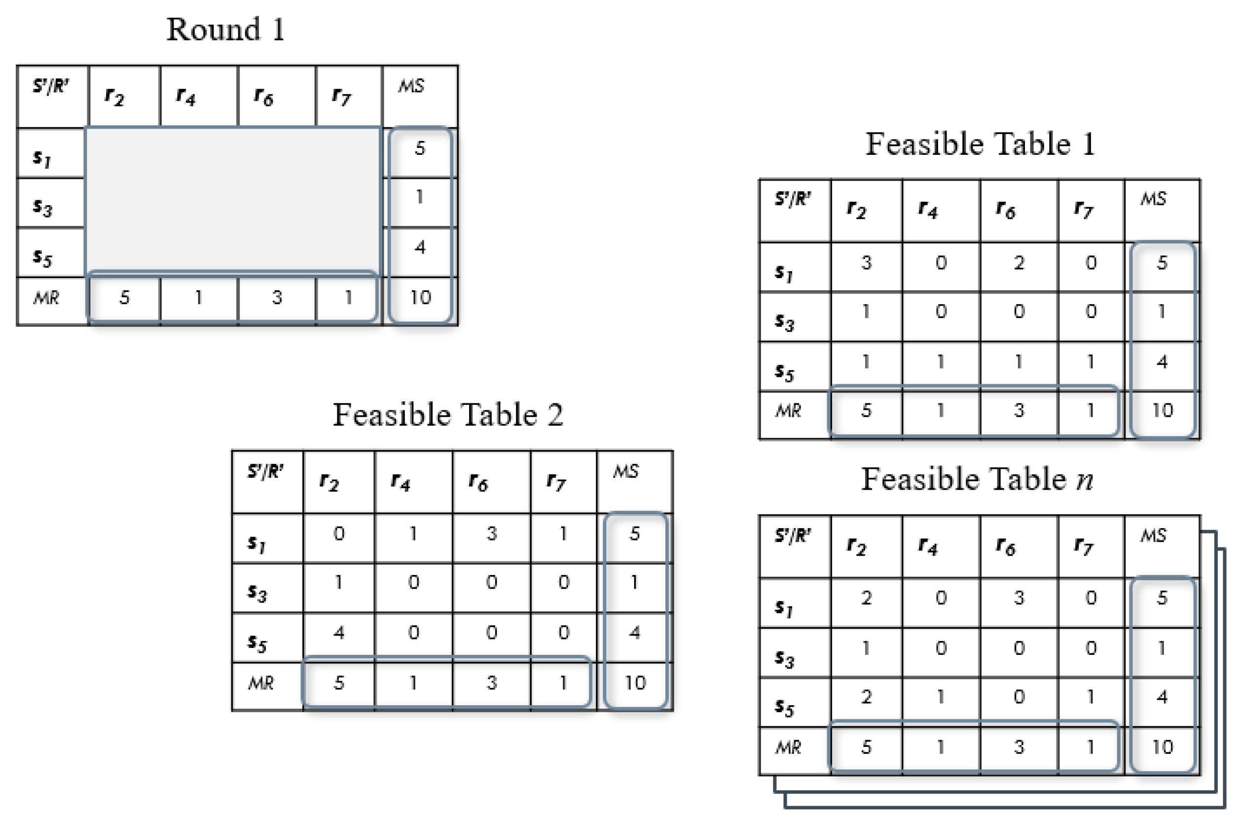
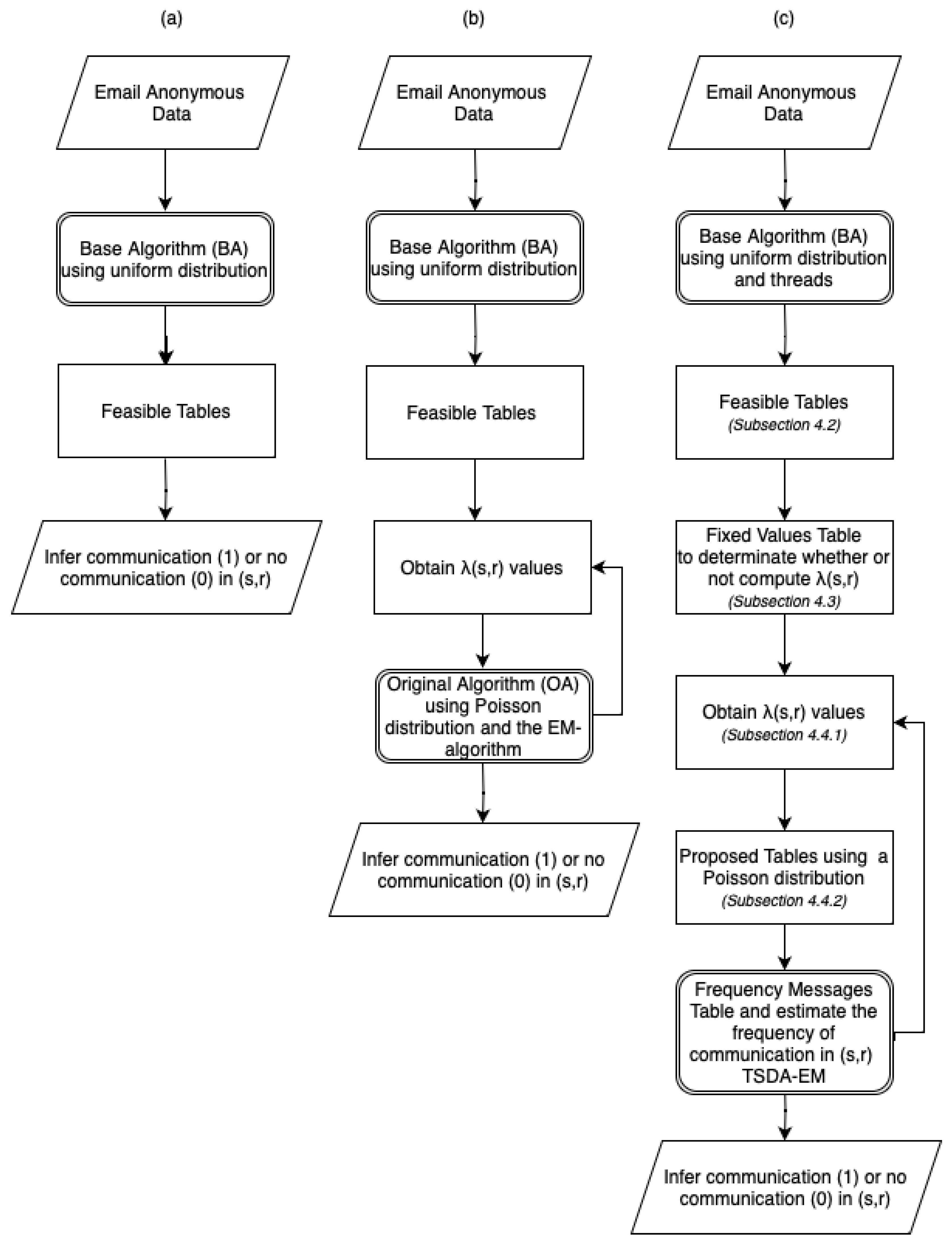
Proposed tables are defined as a set of tables with the same properties as rounds. This means that for each round, there will be a proposed table. The difference from each other is that rounds only contains participants and $marginals$. Otherwise, proposed tables, besides the participants and marginals, will contain a specific cell value that is more likely to be the real number of messages sent by a pair of senders and receivers. A proposed table is an inference generated by a set of Poisson distributions ${\lambda }_{s,r}$, where each cell value (number of messages) has a high probability of being the real number of messages sent and received by the pair of communication. The more refined ${\lambda }_{s,r}$ for each cell is, the more accurately the proposed tables will describe the communication in a round. These proposed tables will also help to remove those excess 1s from the fixed values table. Since the fixed values table (Table 3) knows which communication pair has a 1 (which means, the corresponding cell on every round where this pair appears must have assigned a value different to 0), we can remove such 1 when we finish the proposed table and the cell $[s_i,r_i]$ does not have a value different to 0. That is, the fixed values table for pair $[s_i,r_i]$ recommends putting a value different from 0, but the proposed table was complete with no need to assign a value for this cell. The final objective of these tables is to infer each round with no random values in every cell.

Table 4. Round with its marginals. The “x” in a cell represents a value that needs to be set.

${\mathit{S}}^{\prime }\setminus {\mathit{R}}^{\prime }$	${\mathit{r}}_2$	${\mathit{r}}_4$	${\mathit{r}}_6$	${\mathit{r}}_7$	MS
$s_1$	x	x	x	x	5
$s_3$	x	x	x	x	1
$s_5$	x	x	x	x	4
MR	5	1	3	1

is an example of how to set each value.

Now notice that we have to put in a great effort to complete the tables, assigning values for every cell. For example, in the column of $r_7$, we must set three values for each cell, but only assigning a 1 on the column will complete that row. So the other two cells of the column can be set to 0. In the same way with the sender $s_3$ and recipient $r_4$.

It is important to find the most appropriate value for each cell that does not exceed the $marginals$. This means selecting a random number that falls between the lowest and highest possible values for each cell according to the $marginals$. Additionally, this number must take into account the values stored in the other rows. The BA introduced at [17] runs first and obtains all feasible tables. Then, a rate parameter must be calculated. This parameter, denoted as ${\lambda }_{s,r}$, represents the probability that there is communication between a sender s and a receiver r. It follows a Poisson distribution and needs to be calculated for each cell across the rounds.

The ${\lambda }_{s,r}$ is the number of messages delivered by sender s to recipient r in every round, and it follows a Poisson distribution. It is motivated because rounds constructed by the attacker are based on batches of messages or time periods. The Poisson distribution is a discrete probability distribution, through which it is possible to know the probability that, within a large sample and during a certain interval, an event whose probability is small will occur. Through this methodology, the number of messages delivered by a sender s in a round will follow a Poisson distribution with parameter ${\lambda }_s$. And the number of messages received by recipient r in a round is defined with parameter ${\lambda }_r$. Of course, pairs of users $r,s$ that do not communicate will have a value ${\lambda }_{s,r}$ = 0.

4.4.1. Getting ${\lambda }_{s,r}$ with EM

The Expectation Maximization (EM) algorithm has been used to estimate the means of k normal distributions for the hidden variables $Z=\{z_{i1},\cdots ,z_{ik}\}$, given its current hypothesis $\{{\mu }_{i1},\cdots ,{\mu }_{ik}\}$ and the data $X=\left\{x_i\right\}$. The description of each instance can be thought of as the triplet $\{x_i,z_{i1},z_{i2}\}$, where $x_i$ is the observed value of the ith instance and where $z_{i1}$ and $z_{i2}$ indicate which of the two Normal distributions was used to generate the value $x_i$ [39].

The EM algorithm searches for a maximum likelihood hypothesis by repeatedly re-estimating the expected values of the hidden variables $z_{ij}$ given its current hypothesis $\{{\mu }_{i1},\cdots ,{\mu }_{ik}\}$.

As mentioned before, we use the Poisson distribution ($\lambda$), instead of the normal distribution ($\mu$), motivated by the fact that the rounds, defined by the attacker, may be constructed by batches of messages or, alternatively, by time periods; this distribution is very useful when dealing with unpredictable events.

The EM algorithm consists of two steps:

• Step 1: Calculate the expected value $E\left[z_{ij}\right]$ of each hidden variable $z_{ij}$, assuming the current hypothesis $h=\{{\lambda }_1,{\lambda }_2\}$ holds.
• Step 2: Calculate a new maximum likelihood hypothesis $h^{\prime }=\{{\lambda }_1^{\prime },{\lambda }_2^{\prime }\}$, assuming the value taken on by each hidden variable $z_{ij}$ is its expected value $E\left[z_{ij}\right]$ calculated in Step 1. Then replace the hypothesis $h=\{{\lambda }_1,{\lambda }_2\}$ by the new hypothesis $h^{\prime }=\{{\lambda }_1^{\prime },{\lambda }_2^{\prime }\}$ and iterate.

In the context of our problem, where we have rounds where each one has cells $[s,r]$ and where for each cell we have the number of messages sent (all taken by feasible tables) and its $marginals$, the EM algorithm will be implemented as:

• Hypothesis $h_{s,r}=\{{\lambda }_1,{\lambda }_2\}$, where the initial value for ${\lambda }_1$ is the highest marginal and ${\lambda }_2$ is the lowest marginal of the pair of communication between sender s and recipient r. In case the marginals are the same, ${\lambda }_2$ will be 0.
• Data $X_{s,r}=\{x_1,\dots ,x_i\}$, where $x_i$ will be the number of messages for the cell $[s,r]$ of every feasible table generated for the round on turn.

In order to calculate the expected value $E{\left[z_{ij}\right]}_{s,r}$, the first step will be:

$$E{\left[z_{ij}\right]}_{s,r}={\displaystyle \frac{\frac{{\lambda }_j^{x_i}{e}^{-{\lambda }_j}}{x_i!}}{{\sum }_{n=1}^2\frac{{\lambda }_n^{x_i}{e}^{-{\lambda }_n}}{x_i!}}}$$

(4)

Finally, to calculate a new maximum likelihood, we use:

$${\lambda }_j={\displaystyle \frac{{\sum }_{i=1}^{m}E{\left[z_{ij}\right]}_{s,r}\times x_i}{{\sum }_{i=1}^{m}E{\left[z_{ij}\right]}_{s,r}}}$$

(5)

For a comprehensive understanding of the Expectation Maximization algorithm implementation, please refer to Algorithms 1 and 2. Additionally, in Algorithm 2, we have chosen to provide a more detailed explanation of the process, as we are simulating an iteration for Table 4 to calculate the values $(s_1,r_1)$.

Algorithm 1 Expectation(x, $\lambda$)

1: $numerator\leftarrow {\displaystyle \frac{{\left(\lambda \right)}^x\times e^{-\lambda }}{x!}}$ 2: $n\leftarrow 1$ 3: while $n\le 2$ do      ▹ go through both hypothesis $\{{\lambda }_1,{\lambda }_2\}$ 4:     $denominator\leftarrow denominator+{\displaystyle \frac{{\left({\lambda }_n\right)}^x\times e^{-{\lambda }_n}}{x!}}$ 5: end while 6: return  ${\displaystyle \frac{numerator}{denominator}}$

Algorithm 2 Maximization(). Simulating an iteration for Table 4 for the cell $[s_1,r_1]$

1: ${\lambda }_1\leftarrow 5$ 2: ${\lambda }_2\leftarrow 0$         ▹ since both marginals are the same 3: $i\leftarrow j\leftarrow 1$ 4: $X\leftarrow [5_1,4_2,4_3,3_4,\dots ]$ ▹ Set of values for cell $[s_1,r_1]$ from Feasible Tables of the round 5: while  $j\le 2$  do 6:     while $i\le X.length$ do 7:         $x_i\leftarrow X_i$ 8:         $expectation=Expectation(x_i,{\lambda }_j)$ 9:         $numerator\leftarrow numerator+expectation\times x_i$ 10:       $denominator\leftarrow denominator+expectation$ 11:     end while 12:     ${\lambda }_j\leftarrow {\displaystyle \frac{numerator}{denominator}}$ 13: end while

As a result of EM, we have obtained two new refined likelihood hypotheses for cell $[s,r]$ ($h_{s,r}={\lambda }_1,{\lambda }_2$). These refined hypotheses represent the mean number of messages for the cell. Since each represents a different mean, we only keep the highest in order to have a mean different from 0. Remember, our goal is to generate proposed tables with the most appropriate cell values.

A value ${\lambda }_{s,r}$ for each cell represents the mean number of messages in all the feasible tables. Once we have generated ${\lambda }_{s,r}$, we can use an algorithm to generate a random value with a Poisson distribution.

4.4.2. Proposed Tables

The proposed tables are auxiliary tables that help to infer real communication. Once we have the ${\lambda }_{s,r}$ values, we use an algorithm to generate random values based on the ${\lambda }_{s,r}$’s [40]. Since the algorithm is based on a Poisson distribution, it is important to iterate the EM algorithm to refine the values of ${\lambda }_{s,r}$. There are two different ways to iterate the TSDA-EM algorithm:

• Reuse previously generated feasible tables: The distribution will not vary due to the constant values of the feasible tables, but it may be difficult to store all these tables.
• Generate new feasible tables at each iteration: The distribution will vary depending of the feasible tables, but these will be deleted after they have been used.

Since the number of rounds and tables can be high, we have decided to follow the second option. That is, generate the feasible tables, compute ${\lambda }_{s,r}$, and then drop all these tables.

Our problem is based on a defined period of time, that is, a mix network by either number of messages or a certain amount of time. We say there were exactly n number of messages sent or delivered during one unit of time (which follows a ${\lambda }_{s,r}$) where the inter times $T_1,T_2,\dots$ are exponentially distributed with the rate ${\lambda }_{s,r}$. It can be interpreted as the number of messages sent or received from a Poisson arrival process in one unit of time. And following these ideas, there is a relationship between the Poisson distribution and the exponential distribution. There were n number of messages during one unit of time, but the nth message occurred before time 1; the event $(n+1)$st occurred after time 1. It means the sum of the times $T_1,\dots ,T_n$ belongs to the first unit of time, while the sum $T_1,\dots ,T_{n+1}$ belongs to a second unit of time.

$$T_1+T_2+\cdots +T_n\le 1<T_1+T_2+\cdots +T_{n+1}$$

(6)

Equation (6) can be expressed as

$$\sum _{i=1}^n{T}_i\le 1<\sum _{i=1}^{n+1}{T}_i$$

(7)

As mentioned before, $T_i$ represents the inter times between events (emission and receptions of messages), and it had an exponential distribution with rate ${\lambda }_{s,r}$. We can use the cumulative distribution function in order to generate a probability.

$$F_T\left(T_i\right)=1-e^{-{\lambda }_{s,r}{T}_i}=P_i$$

(8)

As $P_i$ is the probability (it has a uniform distribution over interval $[0,1]$) of the cumulative distribution function $F_T\left(T_i\right)$, we can generate its inverse $F_T\left(T_i\right)=P_i$ for $T_i$ in terms of $P_i$:

$$T_i=F_T^{-1}\left(P_i\right)=-{\displaystyle \frac{1}{{\lambda }_{s,r}}}ln(1-P_i)$$

(9)

A common simplification of Equation (9) is to replace $1-P_i$ by $P_i$ to yield. Now we can define Formula:

$$\sum _{i=1}^n-{\displaystyle \frac{1}{{\lambda }_{s,r}}}ln\left(P_i\right)\le 1<\sum _{i=1}^{n+1}-{\displaystyle \frac{1}{{\lambda }_{s,r}}}ln\left(P_i\right)$$

(10)

Finally, in order to simplify Formula (10), multiply by $-{\lambda }_{s,r}$, use the fact that a sum of logarithms is the logarithm of a product, and then use relation $e^{lnx}=x$ to obtain:

$$\prod _{i=1}^n{P}_i\ge e^{-{\lambda }_{s,r}}>\prod _{i=1}^{n+1}{P}_i$$

(11)

An acceptation-rejection technique to generate random values using Equation (11) with ${\lambda }_{s,r}$ as a parameter is shown in [39]. It has three steps:

• Step 1 set $n=0$, $P=1$
• Step 2 Generate a random number $P_{n+1}$ (over interval [0, 1]), and replace P by $P\ast P_{n+1}$
• Step 3 If $P<e^{-\lambda }$, then accept n. Otherwise, reject the current n, increase n by one and return to step 2.

What these steps do is count the number, n, of random values (probability $P_{n+1}$) generated and stop when the multiplication of these random values, P, is less than $e^{-{\lambda }_{s,r}}$, because this represents that an event occurred in the second unit of time (the right part of Equation (11)). Otherwise, we continue generating random values that belong to the first unit of time. More details of Equation (11) implementation are discussed in Algorithm 3.

In order to generate the proposed tables, it is necessary to identify the cell with the highest ${\lambda }_{s,r}$ and generate a random value for that cell using Equation (11). This value must be truncated to fit within the marginals or can take the value 0.

We have generated a value for the highest ${\lambda }_{s,r}$ to try to complete at least the row or the column and avoid the use of the rest of ${\lambda }_{s,r}$’s in the row or column of this cell. For example, the highest ${\lambda }_{s,r}$ value in

Table 5. Rate parameter (${\lambda }_{s,r}$) for each cell in the round.

${\mathit{S}}^{\prime }\setminus {\mathit{R}}^{\prime }$	${\mathit{r}}_2$	${\mathit{r}}_4$	${\mathit{r}}_6$	${\mathit{r}}_7$	$\mathit{MS}$
$s_1$	3.96	0.99	2.96	0.96	5
$s_3$	0.98	0.46	0	0.70	1
$s_5$	3.95	0.91	2.96	0.96	4
$MR$	5	1	3	1

is cell $[s_1,r_2]$ with ${\lambda }_{1,2}=3.96$. Using Equation (11), it returns the random value 5. A perfect value to complete the $marginals$ of the column and the row.

Algorithm 3 Equation (11) implementation to generate random values given a Poisson distribution ($\lambda$)

1: $n\leftarrow 0$ 2: $P\leftarrow 1$ 3: while $True$ do 4:     $P_{n+1}\leftarrow GetRandomBetween(0,1)$ 5:     $P\leftarrow P\times P_{n+1}$ 6:     if $P<e^{-\lambda }$ then 7:         return n 8:     else 9:         $n\leftarrow n+1$ 10:     end if 11: end while

Since the random value generated completes the row and column marginals, the ${\lambda }_{s,r}$’s for the rest of the row and column are considered unnecessary, and we can assign a value of 0, as shown in

Table 6. Calculated values after the first iteration.

S’/R’	${\mathit{r}}_2$	${\mathit{r}}_4$	${\mathit{r}}_6$	${\mathit{r}}_7$	MS
$s_1$	5	0	0	0	5
$s_3$	0	0	0	1	1
$s_5$	0	1	3	0	4
MR	5	1	3	1	10

. Once we have generated a random value for the highest ${\lambda }_{s,r}$, we can use the fixed values table (Table 3) and generate a value in the cell $[s_i,r_i]$ of the proposed table indicated by the fixed values table only if there is a 1 in cell $[s_i,r_i]$ of the fixed values table. Remember, if there is a 1, it means that a pair of communication has been active the whole time; the value in the cell $[s_i,r_i]$ of the round has to have a number of messages different from 0. In this way, we can continue generating a random value for the cells $[s_i,r_i]$ in the round. Obviously, not all 1s in the fixed value tables are accurate; some of them are wrong. Identifying these wrong 1s is simple; when you do not require the generation of a random cell value, we say the 1 is wrong and does not have a reason to exist. So we change the 1 to 0 on the fixed value table in order to discard it and do not try to generate another random value for the cell in a next iteration. Following the example, these unnecessary cells so far are: $[s_1,r_4]$, $[s_1,r_6]$, $[s_1,r_7]$, $[s_3,r_2]$, and $[s_5,r_2]$.

If those pairs of communication were not used to generate a random number, then we have to change the cell value of the fixed values table to 0 (if there is a 1 on some of the cells of the round). In this way, we can reduce the excess of 1 s from our fixed values table. Those 1 s on fixed table values tell us if we need to assign a value to the cell $[s_i,r_i]$. As we did not assign a value to the cell, it means the cell in fixed table values could be wrong.

Also, there is a possibility to find some rounds where the marginals are not complete. After assigning values to each necessary cell, we check if all marginals are complete. If some marginal are not complete, we must assign a value to complete them. The reason for that is the ${\lambda }_{s,r}$. Because it is too low, it cannot generate at least one value different from 0. Remember that each ${\lambda }_{s,r}$ is refined in function of the values on the cell of each feasible table. If most of the cell values are 0, the ${\lambda }_{s,r}$ will be modeled close to 0. Another reason may be the deactivation of the cell in the last iteration. Due to the disabled cell, it returns 0 by default. For both cases, we must assign a value to complete the table, change the value for the fixed values table, and then activate the cell to get ${\lambda }_{s,r}$. After the first iteration, we obtain Table 6.

5. Results

Previously, we discussed that the number of rounds depends on the threshold set by the mix network for each faculty. This refers to the total number of messages sent and received per round. Table 1 shows the threshold by faculty. The threshold affects the number of rounds by faculty. If a faculty contains a high threshold, the number of rounds will be reduced while the number of senders and recipients by round increases. Conversely, if the threshold is low, the number of rounds will increase while the number of senders and recipients will be reduced by round. A high number of senders and recipients by round means a high computational time and a low classification rate. Remember that we have generated the first feasible tables with random values using the BA [17], so a high number of participants by round will increase the number of feasible tables.

As a result of this proposal, we have achieved the following outcomes. It is important to note that the TSDA-EM algorithm is iterative. As mentioned earlier, after obtaining the initial results by applying the BA [17], we ran our TSDA-EM algorithm several times to improve the results. Most of the time, the classification rate improves with each iteration. In Figure 5, we present the results obtained using TSDA-EM (as described in this work) and the one used in [16], which we refer to as the OA. In this proposal, regarding the classification rate, we found that the best rate was achieved after the second iteration. Therefore, we limited all our experiments to a maximum of four iterations, as shown in Figure 6. The total time taken by the TSDA-EM algorithm must be multiplied by four; e.g., in Figure 7, the time reported is for just one iteration. In the TSDA-EM algorithm, the time for each iteration is exactly the same. Results shown in Figure 5 and Figure 7 were obtained by conducting the experiment with a personal computer with the following hardware specifications: CPU Intel Core i5-8300H, 4.00 GHz, 16 GB DDR4 RAM, and 500 GB HDD.

The TSDA-EM algorithm does not yield improved results when iterated more than five times. As shown in Figure 6, the classification rate stabilizes after ten iterations for one faculty. Each iteration requires the same computational time, which is another advantage of TSDA-EM, as it avoids repeating feasible tables. Previous implementations, based on successive random rearrangements of rows and columns, often resulted in repeated feasible tables [16], consequently increasing computational time.

To complement our results, we have considered a binary classification, where a zero in cell ($s_i$,$r_i$) means no communication, and a value of 1 means that we have inferred communication between user $s_i$ and $r_i$. There are several metrics for binary classification; in this work, we are taking sensitivity and specificity. The first one, sensitivity or true positive rate (TPR), regards the number of cells properly classified to be positive, divided by the number of positive communication. In other words, we measure how many positive cases we have detected. Additionally, we have calculated the opposite quantity of sensitivity, specificity, or true negative rate (TNR). This means that with a high specificity rate, we can confidently state that pairs of senders and recipients who are not communicating are indeed not communicating.

To generate the specificity and the sensitivity metrics we used the proposed tables. As the proposed tables are trying to recreate or infer the real communication, they contain the frequency of communication between every pair of communication in each round. We can take all the proposed tables and generate a table of the whole set of senders S and recipients R as the fixed values table. At this time, this table will not have just two types of values (0 and 1). This table will contain the sum of all messages of the proposed table. One by one, we will sum the number of messages of the same cells. For example, considering Table 6, we have added the values of the cells $[s_1,r_2]$, $[s_3,r_7]$, $[s_5,r_4]$, and $[s_5,r_6]$ to our table. After adding these messages, we will obtain

Table 7. Frequency messages table.

${\mathit{S}}^{\prime }\setminus {\mathit{R}}^{\prime }$	${\mathit{r}}_1$	${\mathit{r}}_2$	${\mathit{r}}_3$	${\mathit{r}}_4$	${\mathit{r}}_5$	${\mathit{r}}_6$	${\mathit{r}}_7$	⋯	$\mathit{MS}$
$s_1$	-	5	0	0	0	0	0	0	⋯
$s_2$	0	-	0	0	0	0	0	0	⋯
$s_3$	0	0	-	0	0	0	1	0	⋯
$s_4$	0	0	0	-	0	0	0	0	⋯
$s_5$	0	0	0	1	-	3	0	0	⋯
$s_6$	0	0	0	0	0	-	0	0	⋯
$s_7$	0	0	0	0	0	0	-	0	⋯
⋮	0	0	0	0	0	0	0	-	⋮
$MR$	⋯	⋯	⋯	⋯	⋯	⋯	⋯	⋯

.

It was only the first proposed table (first round). If other proposed tables contain the same pair of communication (for example $[s_1,r_2]$), we only have to add the number of messages (from the proposed table) to the frequency messages table; see Table 7.

The objective of the previous work is to identify whether or not there is communication between pairs, where 0 means there is not communication and 1 means that it is. In this work, we have estimated the frequency of communication among senders and recipients; see Table 7. Therefore, this is another contribution of the proposed TSDA-EM algorithm.

Nevertheless, in order to compare the performance with previous works, we use Table 7 with binary values, i.e., we set 1 if there is communication and we set 0 otherwise.

We have a dataset with the number of messages among senders S and recipients R for each faculty, which is our ground truth, also called real table [16].

So, the classification rate, specificity, and sensitivity were generated as follows with the real table versus frequency messages table (Table 7):

• True positive (TP): number of messages in both cases is 1.
• False negative (FN): there is communication in the pair of communication but we could not determinate it.
• True negative (TN): number of messages in both cells is 0.
• False positive (FP): there is not communication in the pair, but we have inferred a number of messages.

$$Sensitivity={\displaystyle \frac{TP}{TP+FN}}$$

(12)

$$Specificity={\displaystyle \frac{TN}{TN+FP}}$$

(13)

$$Classificationrate={\displaystyle \frac{TN+TP}{TN+TP+FN+FP}}$$

(14)

Figure 8 shows the specificity rate for each faculty used in this proposal while Figure 9 shows the sensitivity for each faculty. In this way, we state TSDA-EM is better at inferring users who do not communicate for sure. Although the choice between having higher specificity or sensitivity depends on the context and the objectives of the problem. If we consider a scenario where it is more important to avoid errors in identifying negative cases, a high specificity should be prioritized. Conversely, if it is better to correctly detect all positive cases, sensitivity should be prioritized.

After many tests, we notice a better classification rate for each faculty, but after some iteration, the rate does not increase. So checking the proposed tables, we found out that the program gets “stuck.” It generates the proposed tables in the best way that it can. That is, assigning values and completing tables. But it can not notice the wrong assigned values on the cells because apparently there is not any problem with the values on the cells. Look at

Table 8. Real values for the first round of faculty 1.

${\mathit{S}}^{\prime }\setminus {\mathit{R}}^{\prime }$	${\mathit{r}}_2$	${\mathit{r}}_4$	${\mathit{r}}_6$	${\mathit{r}}_7$	$\mathit{MS}$
$s_1$	5	0	0	0	5
$s_3$	0	1	0	0	1
$s_5$	0	0	3	1	4
$MR$	5	1	3	1	10

and compare it with Table 6.

What is the difference between both tables? First, both tables are correct, but Table 8 is the real round. The difference is just one value at the cells $[s_3,r_4]$ and $[s_5,r_7]$. Pay attention to ${\lambda }_{3,4}$ and ${\lambda }_{5,7}$; see Table 5. How do we notice that the value is not in the correct cell? This is why we say that program gets “stuck.” The solution that can solve this problem is the generator of feasible tables where the values of each cell are uniform and not random just to complete the marginals. Maybe taking the proposed tables as feasible tables could be a solution. Remember, if the ${\lambda }_{s,r}$ is wrong, you will finish where you started.

6. Discussion

This study introduces the TSDA-EM algorithm as an improvement over previous approaches to infer communication patterns within an anonymous communication networks. Unlike many prior works that rely on assumptions of uniform communication behavior or homogeneous user groups, the method presented here is designed to accommodate variations in user interaction frequency and social network structures, thereby addressing some of the limitations in earlier algorithms.

Table 9. Comparison of SDA algorithms.

Attack	Accuracy	Friends	Data Used	Mix Network Threshold
PMDA [29]	62%	No restrictions	Synthetic	100
LSDA [32]	90%	25	Synthetic	2–40
RSDA [31]	50%	10	Synthetic	100–500
NSDA [34]	63%	20	Synthetic	10
HSA [28]	95%	23	Synthetic	-
BT-SDA [30]	95% a	No restrictions	Synthetic	20
TSDA-EM [this]	>94%	No restrictions	Real data	10

^a Alice’s friends only.

provides a comparison between TSDA-EM and some of the methods described in the Related Works section of this article. The accuracy column shows there are two distinct sets of algorithms: the ones that achieve less than $65\%$ accuracy and those with more than $90\%$ of this same metric. TSDA-EM belongs to this latter group. Another classification can be made when comparing the number of friends that the Alice user is allowed to have in each study. Some only permit a restricted number, less than or equal to 25, while others have practically no restrictions about this parameter. When considering the previous two metrics, only BT-SDA [30] and TSDA-EM belong to both groups.

The last column compares the threshold value for the mix network employed at each study. A small value implies that fewer messages need to be stored at the mix network before resending them to the intended users, which also means that it becomes easier to identify the relationship between sender and receiver. Conversely, larger values generate more data to be processed by the corresponding algorithm. Given that none of the algorithms in Table 9 are linear, the time and processing complexity rapidly increase with the threshold value. Although the threshold value used in the current study is not large, it is still within the range of other similar studies.

The proposed TSDA-EM algorithm consistently produces favorable results in terms of accuracy while avoiding restrictions in the number of friends for the Alice user. It is important to remember that previous approaches have limited the complexity of user behaviors to create simplified and overly controlled test scenarios, while TSDA-EM has been rigorously tested across varied and more realistic datasets. Moreover, TSDA-EM does not require assumptions about message size, resulting in greater accuracy and robustness across these diverse datasets.

7. Conclusions

This research introduces a new threading statistical disclosure attack with an EM algorithm called TSDA-EM. Our dataset is composed of emails from the Complutense University of Madrid, Spain. According to the best of our knowledge, there are no works using real-world social data in this kind of attack. We have improved the classification rate and the computational time, and we obtained better results to infer who is communicating in an anonymous social network using a mix network. Compared with previous research, we have several contributions: (i) We have developed an iterative algorithm to refine the value of ${\lambda }_{s,r}$ to obtain a better classification rate; (ii) we reduced the time that it takes for each iteration because the TSDA-EM avoids repeated feasible tables; and (iii) we have reduced the total execution time, five times on average, using data with a large number of participants. This computational time reduction is thanks to integrating threads to generate feasible tables, regardless of whether a round has a large number of participants. We have limited the number of combinations for each table. Using multi-threading is a way to perform parallelism by running the threads simultaneously; (iv) we have detected more than 79% of users’ communications in huge networks and more than 95% in small ones. The execution time increases if the number of a round in a faculty is too large because we compute all rounds; (v) moreover, we have inferred the frequency of messages between users (s,r). More than just letting a binary value where 1 indicates communication and 0 no communication, we proposed how many messages have been sent; see Table 7.

For future work, we have identified several research lines to pursue: (i) Instead of assigning random cell values, we propose using the estimated ${\lambda }_{s,r}$ to improve the generation of feasible tables, thereby reducing execution time considerably. (ii) We plan to explore different datasets, such as the Enron Corpus (http://enrondata.org/, accessed on 25 November 2024), to evaluate the performance of the proposed algorithm. (iii) We would like to test time-mix instead of threshold-mix to compare performance. (iv) Besides the EM algorithm, there are other clustering algorithms in the literature that have not yet been studied and could potentially enhance our approach.