Non-Cooperative Target Ranging Based on High-Orbit Single-Star Temporal–Spatial Characteristics

Abstract

A visible light camera payload with star-sensitive functionality was installed to measure the distance between a non-cooperative target satellite and a high-orbit satellite. The rotation matrix was used to calculate the pointing vector from the center of the satellite’s star-sensitive camera axis to the target satellite. Multiple position imaging was achieved, and the moving window approach was used to establish two sets of equations relating the pointing vectors to the positions of binary satellites. To simplify the calculations, the target satellite’s eccentricity was assumed to be small (0 to 0.001), allowing elliptical orbits to be approximated as circular. Additionally, short-interval (1-min) imaging measurements were taken, assuming a small inclination of the target satellite (0.0° to 0.4°). This resulted in the construction of a ranging model with high accuracy, producing a ranging error of less than 5% of the actual distance.

1. Introduction

For situational awareness in space, perceptual measurements of threatening targets, such as space debris, are important safety measures [1,2,3]. In particular, distance measurements of non-cooperative threat targets are critical [4,5]. Visual ranging between two high-orbit satellites requires the host satellite to continuously track and measure the distance to the perceived non-cooperative target satellite [6].

Traditional visual ranging methods include monocular and binocular visual ranging. Monocular visual ranging typically uses point correspondence calibration to obtain depth information from images [7,8]. This method deciphers the transformation relationship between corresponding points in different coordinate systems. As point correspondence calibration requires a predetermined camera position and orientation, any parameter change necessitates recalibration, limiting the use of method to fixed camera positions [9,10,11]. The applicability of cameras mounted on moving platforms (e.g., a camera mounted on a satellite) is restricted because of changes in camera parameters during motion, which impede accurate ranging.

For spaceborne monocular cameras, the continuous tracking of non-cooperative targets is necessary to ensure that the target remains at the center of the camera [12]. However, pixel displacement cannot be guaranteed. Moreover, because this process involves imaging with a single camera, the construction of a binocular model is unachievable [13], which restricts the application of ranging algorithms.

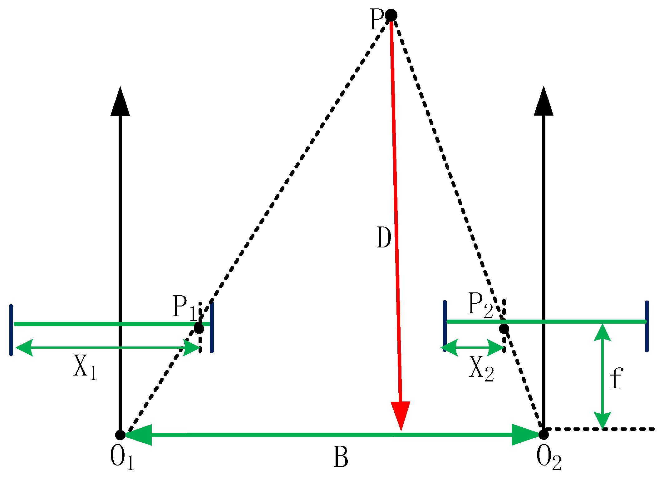
Binocular visual ranging utilizes pixel offsets of the same object on imaging planes to mathematically determine the distance between objects using the camera focal length, pixel offsets, and the actual distance between the two cameras [14,15,16]. The principle of binocular ranging is shown in Figure 1, where $D$ represents the required distance, $f$ denotes the camera focal length, $B$ indicates the center distance between the two cameras, $P$ represents a point on the object, and $O_1$ and $O_2$ are the optical centers of the two cameras. The projections of object point P on the imaging planes of the two cameras are P1 and P2, respectively. By applying the principle of similar triangles (△PO₁O₂∽△PP₁P₂), the distance can be calculated using the formula $D=fB/(X_1-X_2)$, where the focal length ($f$) and center distance ($B$) can be obtained through calibration. Therefore, the distance value can be obtained by determining the value of parallax $d=X_1-X_2$ [17].

In this study, to overcome the limitations of previous methods, we utilized the characteristics of high-orbit satellites in the following ways: (1) spatially—they have low eccentricity and a small inclination angle, which simplifies the motion model of non-cooperative target satellites; (2) temporally—they use the short-term motion of the host satellite to slide and sample pointing vectors continuously to construct a set of equations; and (3), by combining the aforementioned small inclination and short sampling intervals, a further assumption can be made regarding the lack of movement in the Z-axis of the target satellite. Based on these considerations, a monocular visual distance measurement model for non-cooperative targets between high-orbit satellites is proposed.

2. Establishment of the Distance Measurement Model

To obtain monocular visual distance measurements between a host satellite and non-cooperative targets in high Earth orbit, a model for measuring the distance between satellite S and target satellite $\mathrm{T}$ needs to be established. Satellite $\mathrm{S}$ is assumed to be equipped with a star sensor camera capable of real-time tracking and pointing toward the target satellite $\mathrm{T}$. The star sensor camera’s star-sensitive function provides the rotation matrix $\mathrm{M}$ from the celestial coordinate system (which aligns the Z-axis with the Earth’s rotation axis) to the star sensor coordinate system (the star sensor camera can obtain the rotation matrix $M$ through star map matching) [18,19]. The rotation matrix $M_{\mathrm{J}2000}$ from the star sensor coordinate system to the celestial coordinate system is calculated through matrix transposition, as shown in Equation (1).

$$M_{J2000}=M^T$$

(1)

In this paper, the superscript T is used to denote the transpose operation, and the subscript T or t is used to represent the target satellite. Calculating the pointing vector $v_T$ of the onboard camera’s optical axis to the target satellite $\mathrm{T}$ based on the rotation matrix $M_{\mathrm{J}2000}$ from the star sensor coordinate system to the celestial coordinate system can be achieved using Equation (2).

$$v_T=M_{\mathrm{J}2000}U$$

(2)

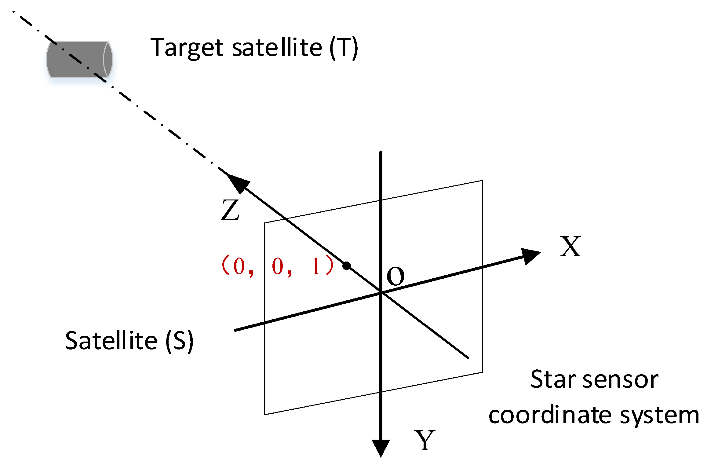
where $U$ represents the vector ${[0,0,1]}^T$. As shown in Figure 2, [0, 0, 1] represents the unit vector in the z-direction of the camera within the star sensor coordinate system. This vector is transformed into the pointing vector of the camera axis to the target within the celestial coordinate system through the ${\mathrm{M}}_{\mathrm{J}2000}$ matrix.

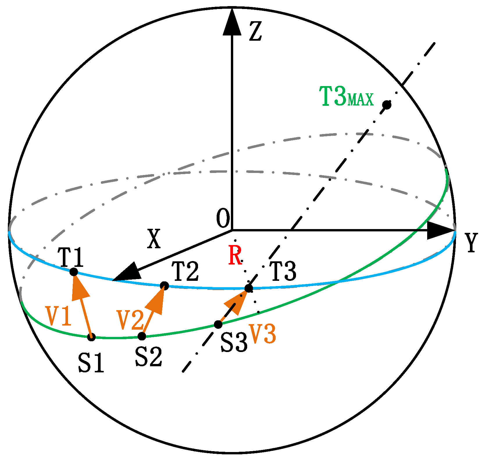
During the ranging process, both satellites are assumed to maintain their respective orbits. The positional changes that occur during the motion of the two satellites are illustrated in Figure 3, in which OXYZ represents the celestial coordinate system. This assumes the movement positions of satellite $S$ in its orbit as $S1$→$S2$→$S3$, and simultaneously, the movement positions of target satellite $T$ in its orbit as $T1$→$T2$→$T3$. Satellite $S$ moves from position $S1$ to position $S2,$ with the coordinates corresponding to these positions denoted as $S1 (x_{\mathrm{s}1},y_{s1},z_{s1})$ and $S2 (x_{\mathrm{s}2},y_{s2},z_{s2})$. When satellite $S$ is at positions $S1$ and $S2$, the assumed coordinates for the corresponding positions of target satellite $T$ are $T1 (x_{\mathrm{t}1},y_{t1},z_{t1})$ and $T2 (x_{\mathrm{t}2},y_{t2},z_{t2})$. At position $S1,$ satellite $S$ points to the position of target satellite $T$ at $T1$; similarly, at position $S2$, satellite S points to the position of target satellite $T$ at $T2$. The corresponding pointing vectors are $v_1(v_{x1},v_{y1},v_{z1})$ and, $v_2(v_{x2},v_{y2},v_{z2})$, which can be calculated using Equations (3) and (4) derived from Equations (1) and (2), respectively:

$$v_1^{\mathrm{T}}=M{1}_{\mathrm{J}2000}U$$

(3)

$$v_2^{\mathrm{T}}=M{2}_{\mathrm{J}2000}U$$

(4)

where $M{1}_{\mathrm{J}2000}$ and $M{2}_{\mathrm{J}2000}$ are the rotation matrices from the star sensor coordinate system to the celestial coordinate system at positions $S1$ and $S2$, respectively.

Assuming the unknown coefficients $k_1$ and $k_2$, we construct the vector equation $v_1$ for satellite $S$ pointing to target satellite $T$ at position $T1$ when $S$ is at position $S1$ and perform a similar construction for vector equation $v_2$.

$$k_1{v}_1=S1-T1$$

(5)

$$k_2{v}_2=S2-T2$$

(6)

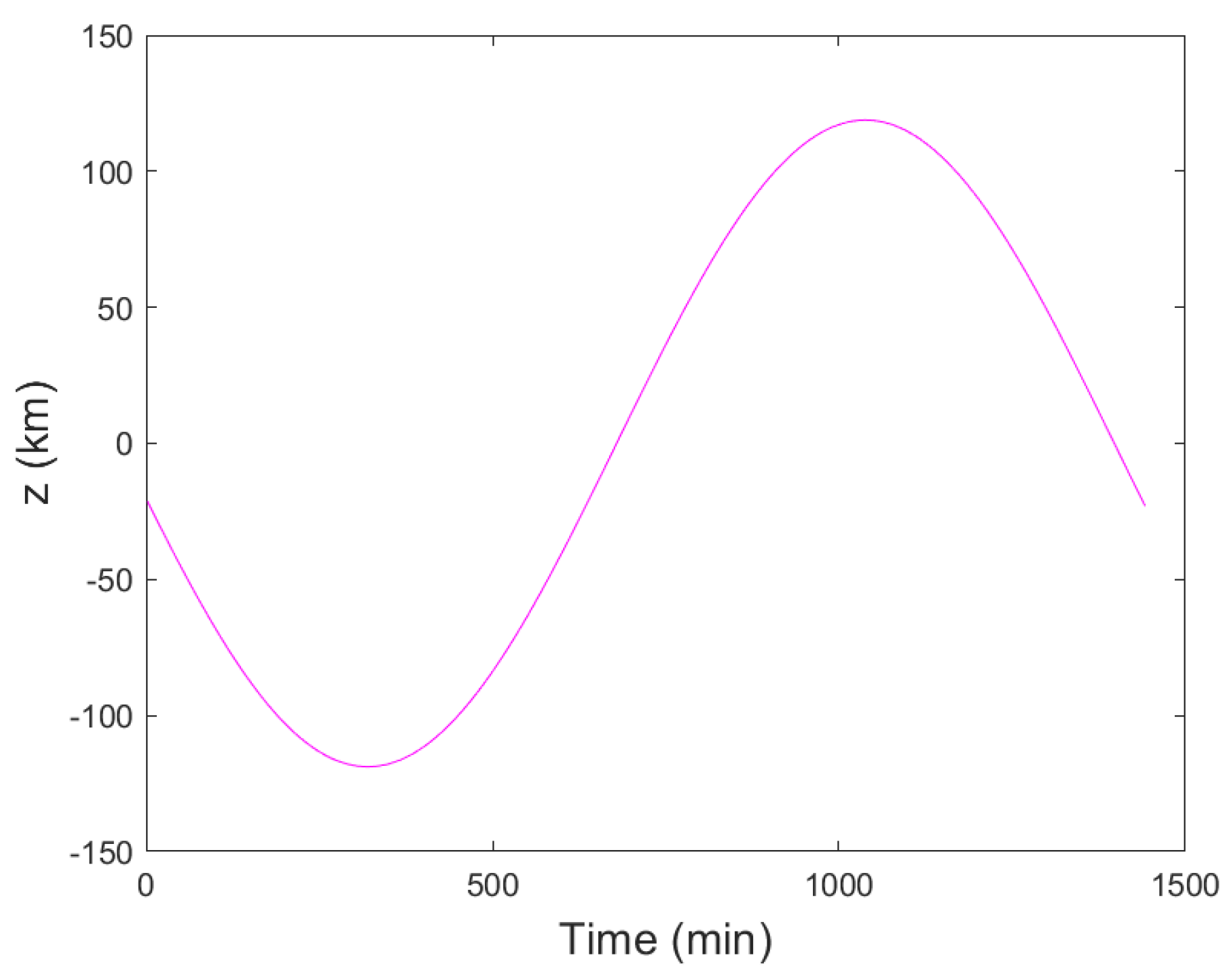
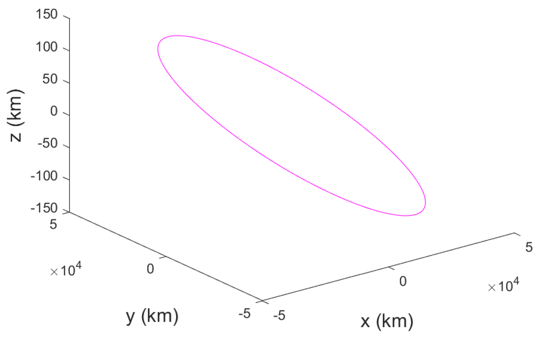
Assuming a short time interval between the two samples (e.g., 1 min) and a near-zero orbital inclination, the motion of target satellite T in the Z-axis direction can be approximated as nearly 0 (the high-orbit target is on a relatively stable orbit with minimal movement in the Z-axis direction) [20,21]. Variation along the Z-axis is illustrated in Figure 4. Figure 5 shows the 24 h orbital Z-axis variation relative to the X and Y-axes. The analysis during ranging, with a 1 min sampling interval, revealed minimal changes in the Z-axis (0.4° inclination within 600 km at 0.2 km/min). Consequently, we assumed Equation (7):

$$z_{t1}=z_{t2}$$

(7)

According to Kepler’s first law, the satellite’s orbit is elliptical [22,23], as shown in Equation (8), where $a$ represents the semimajor axis, $e$ indicates the eccentricity, $r$ denotes the polar radius, and $\theta$ represents the true anomaly, as shown in Figure 6.

$$a(1-e^2)=r(1+e\cos (\theta ))$$

(8)

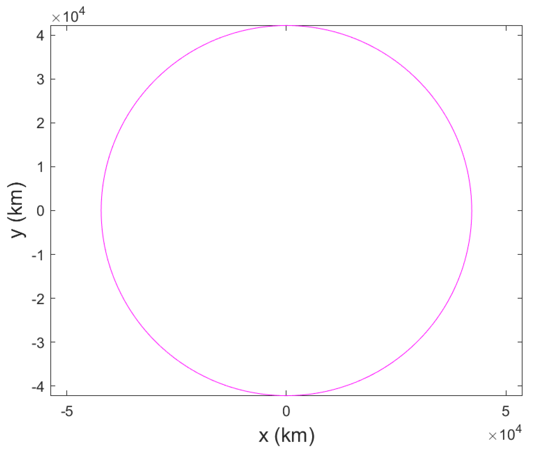
Based on the characteristics of high−orbit satellites, when the eccentricity $e$ is small, the elliptical orbit can be approximated as a circular orbit [24]. Additionally, when the inclination is small, its projection onto the XY plane forms a circular orbit, as shown in Figure 5 and Figure 7. Therefore, an approximation can be made, as shown in Equation (9).

$$x_{t1}^2+y_{t1}^2=x_{t2}^2+y_{t2}^2$$

(9)

Furthermore, the variation in XYZ coordinates in the J2000 coordinate system can be calculated by converting the orbital elements to the J2000 coordinate system. First, the orbital elements are defined as follows: semi-major axis (a), eccentricity (e), inclination (i), right ascension of the ascending node (Ω), argument of periapsis (ω), and mean anomaly (M). Additionally, the eccentric anomaly (E) and true anomaly (f) are defined for the computational process. From Kepler’s equation, we can obtain the following:

$$M=E-e\sin (E)$$

(10)

where the eccentric anomaly (E) can be calculated iteratively from the mean anomaly (M). The satellite’s position in the J2000 coordinate system can be calculated [25]:

$$\left(\begin{array}{c}{x}_{J2000}\\ y_{J2000}\\ z_{J2000}\end{array}\right)={\displaystyle \frac{a(1-e^2)}{1+e\cos (f)}}\left(\begin{array}{c}\cos (\mathsf{\Omega })\cos (\omega +f)-\sin (\mathsf{\Omega })\sin (\omega +f)\cos (i)\\ \sin (\mathsf{\Omega })\cos (\omega +f)+\cos (\mathsf{\Omega })\sin (\omega +f)\cos (i)\\ \sin (\omega +f)\sin (i)\end{array}\right)$$

(11)

Equation (11) includes the exact expression for $z_{J2000}$. When the eccentricity (e) approaches 0, we have the following relationship:

$$z_{J2000}=a\sin (i)\sin (\omega +f)$$

(12)

In this case, a, i, and ω are constants, and the value of f ranges from 0 to 2π. Assuming a short time interval between two samples (e.g., 1 min), it can be considered that the two samples’ true anomaly (f) values are close to each other, leading to small changes in the Z-axis. This gives the expression in Equation (7).

From Equation (11), the following calculation can be performed:

$$x_{J2000}^2+y_{J2000}^2=a^2{\cos }^2(\omega +f)+a^2{\cos }^2(i){\sin }^2(\omega +f)$$

(13)

Furthermore, when i is small, we can approximate that ${\cos }^2(i)=1$, yielding Equation (14):

$$x_{J2000}^2+y_{J2000}^2=a^2$$

(14)

Thus, when the change in the true anomaly (f) is small, the equation can be written as in Equation (9).

Based on Equations (1), (3)–(7) and (9), the coefficient $k_2$ can be solved to obtain the absolute values of the two solutions, $d{1}_{abs}$ and $d{2}_{abs}$. Consequently, Equation (15) can be used to select the minimum coefficient.

$$d=\min (d{1}_{abs},d{2}_{abs})$$

(15)

As shown in Figure 3, when the two satellites move to position 2 (establishing equations using positions 1 and 2), the calculated coefficient $k_2$ for the pointing vector assumes two values. This is the case because, according to Equations (7) and (9), the pointing vector intersects the surface of the cylinder where the target satellite $\mathrm{T}$ is located at two points. The minimum value of the coefficient represents the observable target satellite, and another point is located in a position that cannot be observed in the line of sight. Thus, by selecting the minimum coefficient, the distance from satellite $\mathrm{S}$ to target satellite $\mathrm{T}$ can be determined using Equation (16).

$$d_{last}=d\sqrt{(v_{x2}^2+v_{y2}^2+v_{z2}^2)}$$

(16)

3. Experimental Results

We used simulation software (STK 11.0) to establish a scenario for the primary and target satellites to validate the algorithm proposed in this paper. First, we set the orbital parameters for the primary satellite and the different target satellites. At different times, the orbital parameters of the primary satellite and the pointing vector toward the target satellite are known. The actual distance between the two satellites can be obtained through the simulation software, and this distance serves as the standard answer for validating the algorithm presented in this paper. Our algorithm does not know the orbital parameters of the target satellite. We compared the distance calculated by the algorithm with the standard answer to analyze the algorithm’s error.

The orbital parameters for the host satellite in the ranging experiment were as follows: semimajor axis, 42,166 km; eccentricity, 0.0005; and inclination, 5°. For the target satellite, the corresponding values were as follows: semimajor axis, 42,176 km; eccentricity, 0.0002; and inclination, 0.0°/0.1°/0.2°/0.3°/0.4°/1.0°.

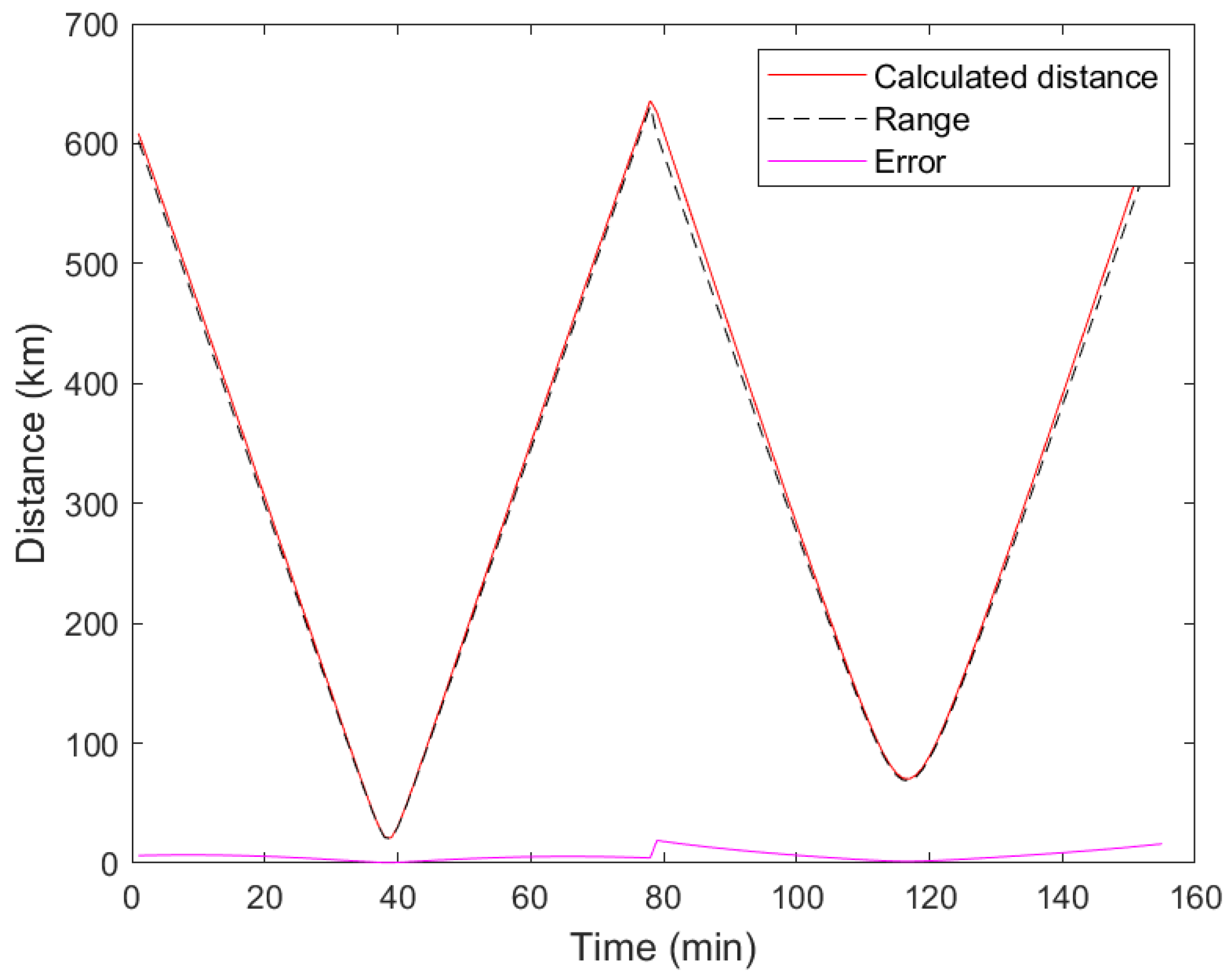
Figure 8, Figure 9, Figure 10, Figure 11 and Figure 12 display the error curves for inclinations of 0.0°, 0.2°, 0.4°, and 1.0°. Ranging accuracy within 600 km was superior to 5% of the detection distance for inclinations between 0.0° and 0.4°. Furthermore, for inclinations between 0° and 1°, a ranging accuracy within 100 km range was guaranteed to be superior to 5% of the detection distance.

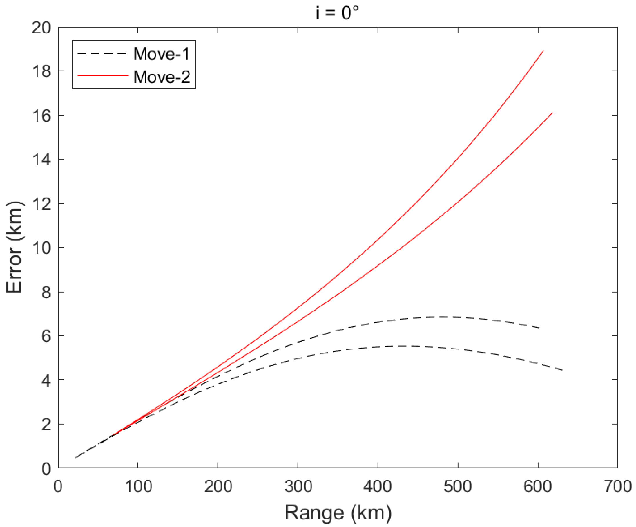
The two “V” shapes occur because the ground track of the host satellite forms a figure-eight shape, resulting in two approaches and two retreat events between the two satellites. In Figure 9, Figure 10, Figure 11, Figure 12, Figure 13 and Figure 14, we represent these two events with the symbols Move-1 and Move-2. Furthermore, we assume that the satellite (S) is an inclined geosynchronous satellite and that the target satellite (T) is a geosynchronous satellite with a small eccentricity (ranging from 0 to 0.001) and a small inclination (ranging from 0.0° to 0.4°). The ground track of the satellite (S) forms a figure-eight pattern, which is the trace created by the line connecting the satellite to the center of the Earth and its intersection with the Earth’s surface. The satellite (S) experiences two approaches and retreats from the target satellite (T), resulting in the red and black lines shown. In Figure 8, the black dots represent the calculated distance values from the model, the red dots represent the actual distances, and the green dots indicate the error.

As shown in Figure 13, under the first set of movements (Move-1), the error curves for different inclinations (0.0° to 0.4°) indicate a gradual reduction in error from 0.0° to 0.2°, followed by a gradual increase from 0.2° to 0.4°, with a maximum error of approximately 10 km at around 500 km. The ranging error is less than 2% of the measured distance. Figure 14 demonstrates that under the second set of movements (Move-2), the maximum error at a distance of 600 km is less than 30 km. The ranging error is less than 5% of the measured distance.

4. Discussion

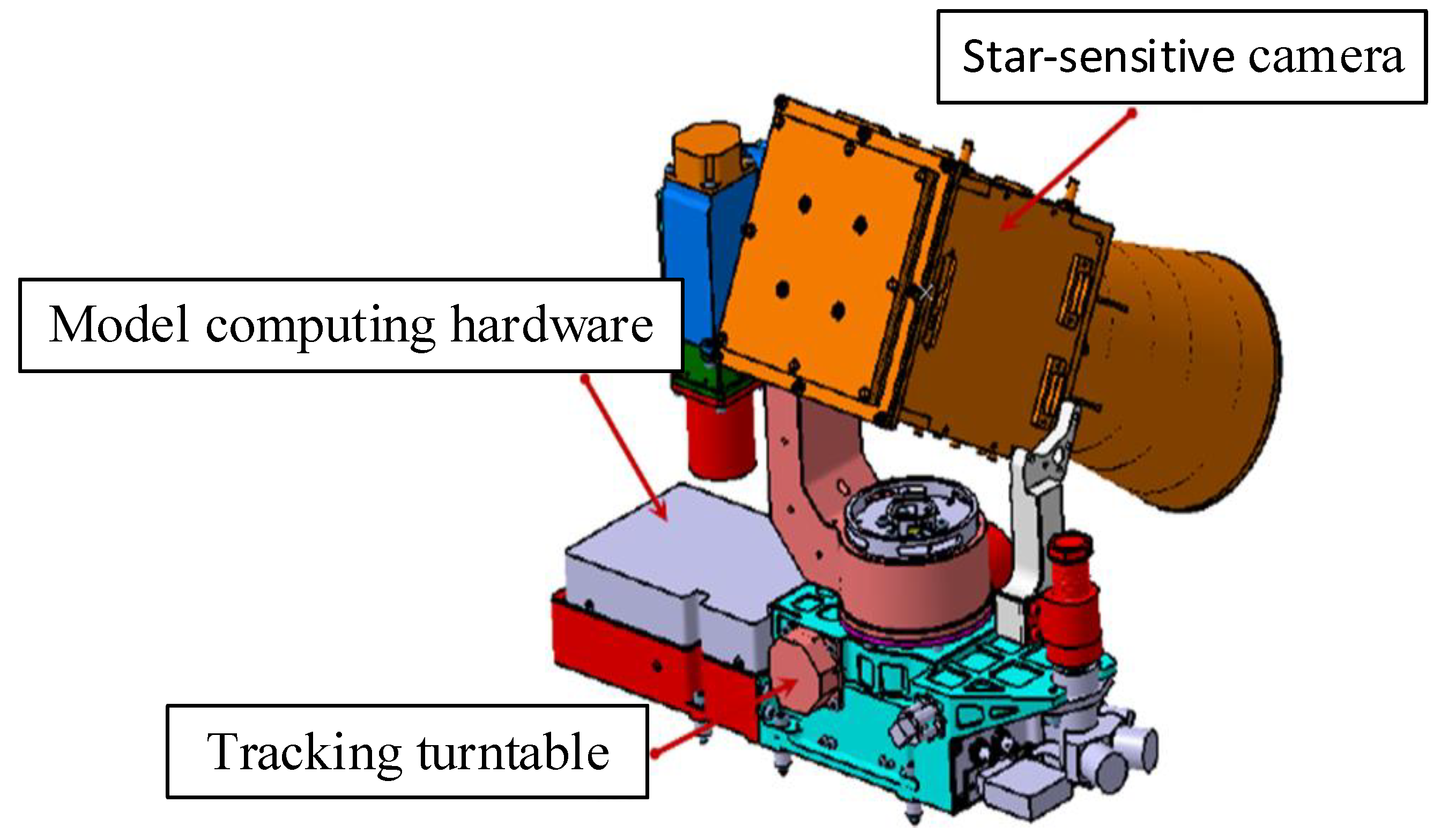
The range model developed herein was successfully deployed on a satellite platform, as illustrated in Figure 15, for the distance measurement of high-orbit threats such as space debris. The system comprises a star-sensitive camera for target acquisition and outputting rotation matrices, a tracking turntable for real-time target tracking, and a field-programmable gate array (FPGA) for computational hardware. The algorithm operates on this hardware platform, leveraging the characteristics of the satellite’s motion and generating continuously changing pointing vectors, as well as its own position. This allows data acquisition at different time intervals. The model calculates the ranging results by continuously sampling two sets of data collected approximately 1 min apart. A sliding sampling method was adopted to compute results every 10 s to ensure real-time calculations.

In Equation (7), an assumption is made that the target satellite’s Z-axis remains unchanged. If we further assume that the distance measurements from two observations are equal (satellite S measures the same distance at S1 and S2), then the distance can be calculated using Equations (17)–(19).

$$z_{s1}-z_{t1}=k_1{v}_{z1}$$

(17)

$$z_{s2}-z_{t2}=k_2{v}_{z2}$$

(18)

$$k_1(v_{x1}^2+v_{y1}^2+v_{z1}^2)=k_2(v_{x2}^2+v_{y2}^2+v_{z2}^2)$$

(19)

These equations rely heavily on the variation in the pointing vector $v_z$ to calculate the result. In practice, $v_z$ is a normalized value, and the change in $v_z$ from two observations is reflected in approximately the sixth decimal place. This situation introduces significant errors in the calculation and proves challenging to implement in an FPGA.

The star map matching process for the star-sensitive camera is conducted in the celestial coordinate system. If all computational processes are shifted to the WGS84 coordinate system, it may be feasible to consider solving the trigonometric relationships through two observations. However, this would entail complex coordinate system transformations and could lead to significant errors in the case of extremely small angles.

In contrast, the proposed model is straightforward, requiring no coordinate system transformations and avoiding significant errors arising from small angles. Instead, errors arise from the assumptions within the equations, and refining these assumptions can further enhance precision.

5. Conclusions

No prior model is available for distance measurement in the continuous tracking process of high-orbit non-cooperative targets. Additionally, the real-time computational resources on the satellite hardware platform are limited. This necessitates the design of a simple yet effective computational model.

This model assumes that the high-orbit satellite is relatively stationary with a low eccentricity and minimal orbital inclination. The designed model was verified using both simulation validation and actual in-orbit testing. Within an inclination range of 0.0° to 0.4°, the ranging accuracy within a 600 km range surpasses the detection distance by 5%, whereas within an inclination range of 0.0° to 1.0°, the ranging accuracy within a 100 km range is guaranteed to exceed the detection distance by 5%.