Characterization of a Mechanical Antenna Based on Rotating Permanent Magnets

Abstract

Mechanical antennas with rotating permanent magnets are a relatively new type of transmitting antenna in low- and ultralow-frequency (LF/ULF) ranges. The perspectives of the applications are encouraging, especially in the field of non-destructive defectoscopy and communications through conductive media (underwater communications), which is reflected in the articles published in the last decade. This article describes the experimental setup, results, harmonic analysis, and simulation validation for two configurations of mechanical antennas with rotating NdFeB permanent magnets. The emphasis is placed on the known analytical equations, specifically on the matching of the measurement results with the analytical data as well as with the results given by the numerical analysis. Also, several means of measurement are used to validate the results through replicate testing. Through analytical analysis and the performed measurement, this article establishes the basics for designing mechanical antennas with rotating permanent magnets for the considered configurations based on a single static magnetic field measurement. Finally, we explore prospects for future research in this domain as well as the advantages and disadvantages compared to other types of LF/ULF antennas.

1. Introduction

Electromagnetic radiation in the extremely low-/super low-/ultralow-/very-low- (ELF/SLF/ULF/VLF)-frequency ranges (3 Hz–30 Hz/30 Hz–300 Hz/300 Hz–3 kHz/3 kHz–30 kHz) has small path losses in harsh electromagnetic environments like soil, sea water, or materials with good electrical/magnetic properties included in the structure of various industrial, military, or civil constructions. This makes them essential in applications like submarine communication, mine emergency communication, and earthquake prediction [1]. However, generating ELF/ULF/VLF electromagnetic waves is a challenge due to the very large wavelengths at these frequencies, which make it difficult to build antennas with adequate dimensions. Moreover, short antennas are ineffective and narrowband due to the low wave impedance and impedance mismatch [2]. Thus, achieving antennas with small dimensions that are effective in the mentioned frequency ranges has become an objective for research teams across the entire world, and the mechanical approach, which involves the mechanical motion of materials that carry electrical charges or of magnetic materials in order to generate low-frequency electromagnetic waves (ELF/ULF/VLF), has proven to be successful.

Miniaturization of very-low-frequency antennas can add underground or collapsed buildings localization, wireless energy transfer, applications within the internet of things (IoT), determining the electromagnetic shielding effectiveness of materials or enclosures, or finding the electromagnetic radiation leakages of a shielded enclosure to the applications list.

This work focuses on the design, construction, and testing of mechanical antennas with rotating NdFeB permanent magnets for generating low-frequency magnetic fields between 30 Hz and 100 Hz.

Neodymium-iron-boron (NdFeB) magnets are instrumental in advancing technology due to their high magnetic strength and energy density. NdFeB magnets are recognized as the strongest type of permanent magnets available today. With a remanence of 1.1–1.2 T, these magnets are pivotal in various high-tech applications, making them a focal point of research and development in material science and engineering. The high remanence indicates a robust capacity for maintaining magnetization, making NdFeB magnets suitable for use in demanding environments and applications [3].

The article describes the mechanical project, the devices and setups used during the measurements, the validation of the numerical analysis through experiments, the determination of the content of harmonics and interharmonics related to the functional emission frequency, the dependence of the field on the distance, the maximum sensitivity obtained in a suburban environment, and the predicted performances for similar, better-performing systems.

2. Related Works

Regarding the structure, antennas with permanent magnets were made in various configurations with one or more parallelepiped or cylindrical permanent magnets with different dimensions, axially or radially magnetized, that have rotating or vibration motion or are fixed with a rotating shutter that enables the alternative passing of the static dipole magnetic field.

Thus, in 2018, Shuhong Gong et al. [1] showed a mechanical antenna with a rotating neodymium permanent magnet that had a remanence of 1.2 T and a rectangular shape with a size of 10 cm × 5 cm × 2 cm (100 cm³ volume). In [4], a cylindrical NdFeB permanent magnet with a diameter of 5 cm and a height of 3 cm was used to generate a low-frequency magnetic signal. The magnet was axially magnetized, and its nominal remanence was 1.2 T. The generated signal had a frequency of 35.6 Hz, and the magnetic field measured at a distance of 2 m was 1500 nT and at 8.4 m was 17 nT.

Yahao Dong et al. [5] proposed a type of mechanical antenna that is based on dual permanent magnets and consists of an actuation module and two neodymium cylindrical permanent magnets radially magnetized with a remanence of 1.25 T and a volume of 3.93 cm³. The experimental results showed that the magnetic flux density reached 2.35 nT at 1 m in air. An application approached by the authors was positioning of and communication with pipeline robots. Thus, the antenna was placed inside a steel pipeline with an outer radius of 180 mm, length of 1200 mm, thickness of 8 mm, and conductivity of 4.22 MS/m. For the Bx component of the magnetic field measured at a distance of 3 m from the pipeline, a value of 40.57 nT without pipeline and a value of 6.59 nT with pipeline were recorded.

Mark Gołkowski et al. [2] presented a mechanical antenna with rotating shutters and fixed permanent magnets. By rotating a shutter with multiple apertures made of a soft magnetic material in front of fixed magnetic dipoles, the static magnetic dipole field is alternately passed or distorted by the shutter. The shutter’s number of apertures, N, reduces the rotating speed required to obtain the desired radiation frequency, ω, to ω/N. Two versions of mechanical antennas were presented with four and eight rectangular neodymium permanent magnets placed around the DC motor that rotates two aligned steel shutters with eight apertures separated by the same distance as the permanent magnets.

In [6], an electromechanical system called a Magnetic Pendulum Array (MPA) was proposed. The array is self-biased; the alignment of each magnet in the array to the array axis occurs by itself due to the field of the adjacent magnets. Around the housing in the plane of the magnets, an external coil is placed to excite the magnets to create a time-varying magnetic field that is perpendicular to the pendulum array plane. The prototype of the magnetic pendulum array consists of 28 pendulum elements suspended by stainless steel ball bearings in a plastic housing. Each pendulum element is made of a diametrically magnetized NdFeB cylindrical magnet with a length of 40 mm and a radius of 4 mm and is supported by aluminum bearing adapter sleeves on each end. The excitation field is provided by a coil that is wrapped around the magnets.

A simulated model of mechanical antenna with rotating magnet was shown in [7]. Two kinds of mechanical motions were studied here: a uniform circular motion around the rotating shaft and a shifting motion. The model used a NdFeB cuboid permanent magnet with a volume of 6 mm³, relative permeability of 1.099, and magnetic coercivity of 8900 kA/m. The simulation showed that very-low-frequency signals below 1000 Hz over a distance of 20 m can be obtained.

Jianqiang Bao et al. [8] reported a mechanical antenna based on a triangular array of rotating permanent magnets. The used NdFeB magnets are cylindrical with a radius of 5 mm and a height of 3 mm and have a residual flux density of 1.23 T. The magnets are fixed on a disc made of an aluminum alloy with a diameter of 100 mm and a thickness of 2 mm. Reference [9] showed a mechanical antenna based on a vibrating permanent magnet. This mechanical antenna radiates electromagnetic waves in the ELF band by an alternate motion of the permanent magnets and can generate an induced voltage with a peak value of 0.179 mV at 1 m.

Another type of mechanical antenna with permanent magnets is the resonant Magneto-Mechanical Transmitter (MMT). The MMTs described in [10,11] use resonant angular oscillatory motion of one or more permanent magnet rotors to produce a ULF signal. This approach was experimentally demonstrated by the authors by using two MMT systems. The first MMT prototype uses a construction with a single rotor that works at 166 Hz and generates a magnetic field of 1.09 fT at 1 km. The second MMT prototype has six identical cylindrical rotors and two cuboidal stators. When they are adequately overlapped, two modules of six rotors can work as a larger MMT system that can produce twice the time-variable field. The magnetic field produced by two modules with six cylindrical rotors has a frequency of 900 Hz and an amplitude of 0.34 fT at 1 km.

Based on the large-volume splitting method, Wenhou Zhang et al. [12] used permanent magnets with small volumes to form a mechanical antenna array. The experimental results show that if a time-variable magnetic field sensor with a sensitivity of more than 100 fT is used to receive the generated signal, the developed prototype has a transmission distance of 700 m. Also, the results show that the best structure of mechanical antenna radiation source is the axially magnetized cylindrical permanent magnet. The magnets used for this mechanical antenna array were 30 mm in diameter and 60 mm in height.

In [13], a magnetoelectric (ME) mechanical antenna based on the magneto-mechano-electric (MME) effect was presented. The MME effect results from the combination between the piezo-driven magnets’ motion and converse magnetoelectricity (ME). The system consists of a fixed PZT/Metglas structure with a permanent magnet attached to its free end. The oscillating magnet is used as an additional vibrating magnetic dipole that improves the radiation of the mechanical antenna. For one of the devices they made, the authors reported, at a frequency of 11.32 kHz, a magnetic field with a measured value of ~0.01 nT at a distance of 5 m.

Mechanical antennas were also built based on the piezoelectromagnetic effect. The piezoelectromagnetic effect was also used to build mechanical antennas. Thus, in order to significantly reduce the dimensions of low-frequency antennas, Yunping Niu and Hao Ren [14] proposed a pair of low-frequency transmitting and receiving mechanical antennas. An AC voltage applied to the transmitter generates an alternating strain and an electromagnetic wave, while by applying an electromagnetic wave to the receiver, an alternating strain and a voltage are generated. Both antennas are made up of a magnetostrictive Terfenol-D and piezoelectric PZT laminate. In order to improve the performances at small dimensions, in both antennas, small Rb magnets that provide a bias DC magnetic field were added. The pair of miniaturized mechanical antennas work at a mechanical resonance frequency of 37.95 kHz, and a signal amplitude of 14.51 µV was obtained at a distance of 9 m.

For the various mechanical antennas involving permanent magnets, Table 1 shows a summary of the measured results extracted from the related literature along with the theoretical model used to calculate the generated magnetic field and the applications these antennas were intended for.

Table 1. Performances of various mechanical antennas with permanent magnets.

Design	Magnetic Field	Frequency	Theory	Applications	Reference
One rotating permanent magnet made from NdFeB, rectangular	1.67 nT @ 0.5 m	30 Hz	Amperian current model	Underwater, underground communications	[1]
	0.25 nT @ 1 m
Rotating shutter, four fixed rectangular NdFeB permanent magnets	1.2 nT @ 1 m	960 Hz	-	Broadband radiation	[2]
	18 pT @ 5 m
Rotating shutter, eight fixed rectangular NdFeB permanent magnets	3.1 nT @ 1 m	960 Hz	-	Broadband radiation	[2]
	44 pT @ 5 m
One rotating NdFeB permanent magnet, cylindrical	1.5 µT @ 2 m	35.6 Hz	Magnetic dipole	Low-frequency magnetic communications in lossy environments	[4]
	17 nT @ 8.4 m
Two rotating NdFeB permanent magnets, ring-shaped, radially magnetized	0.95 µT @ 1 m	30 Hz	Magnetic dipole	Communication through conductive media, such as in pipelines, underwater, and underground	[5]
	2.35 nT @10 m
Magnetic Pendulum Array (MPA) made of 28 NdFeB cylindrical permanent magnets, diametrically magnetized	0.5 nT @ 10 m	1031 Hz	Oscillating magnetic dipole	Efficient generation of ULF radiation	[6]
	0.03 nT @ 30 m
One rotating NdFeB permanent magnet, cuboidal, with a volume of 6 mm3 (simulation)	2 pT @ 1 m	<1000 Hz	Second derivative of magnetic dipole moment versus time	Communications	[7]
	1.4 pT @ 3.5 m
One triangular array of NdFeB permanent magnets	11.8 V @ 0.15 m	15 Hz	Rotating magnetic dipole	Underground and underwater communications	[8]
	0.85 V @ 0.5 m
One rotating NdFeB permanent magnet, rectangular	0.114 mV @ 1 m	5 Hz	Magnetic dipole	Wireless transmission systems	[9]
	0.112 mV @ 1 m	15 Hz
One vibrating NdFeB permanent magnet, rectangular	0.179 mV @ 1 m	5.8 Hz	Magnetic dipole	Wireless transmission systems	[9]
	0.179 mV @ 1 m	6.4 Hz
Resonant magneto-mechanical transmitter (MMT) with one rotor and two stators of NdFeB magnets with square cross section	1 fT @ 1 km (1/r3 extrapolation)	166 Hz	Point dipole with moment Mr	Low data rate communications in conductive or radio-obstructed environments	[10,11]
Resonant magneto-mechanical transmitter (MMT) with 2 × 6 rotors of cylindrical NdFeB magnets and two stators of NdFeB magnets with a square cross section	0.34 fT @ 1 km (1/r3 extrapolation)	900 Hz	Point dipole with moment Mr	Low data rate communications in conductive or radio-obstructed environments	[10,11]
Mechanical antenna array with rotating NdFeB cylindrical magnets, axially magnetized	31.6 nT @ 10 m	75 Hz	Ampere molecular circulation hypothesis	Ultralong-wave communication through the air–seawater interface	[12]
	0.05 nT @ 80 m
Magnetoelectric (ME) mechanical antenna based on a PZT/Metglas fixed structure; one cylindrical NdFeB permanent magnet attached at its free end	~0.01 nT @ 5 m	11.32 kHz	Current loop (for comparison with the ME antenna)	Wireless signal transmission	[13]
Magnetostrictive Terfenol-D and piezoelectric PZT laminate with 4 Rb magnets for DC polarization	2.8 µT @ 5 cm	37.95 kHz	Piezoelectromagnetic effect	Portable electronics and IoT applications	[14]
	13 nT @ 30 cm
One rotating NdFeB permanent magnet, cylindrical, diametrically polarized, suspended between two high-permeability laminated pole pieces	0.6 µT @ 1 m	22 Hz	Basic coil	Communication systems	[15]
One rotating NdFeB permanent magnet, ring-shaped, diametrically magnetized	800 pT @ 10 m	500 Hz	-	Data communication and/or position/navigation/timing in lossy environments	[16]
	800 fT @ 100 m
Transmitter with electrically modulated reluctance (EMR) having one rotating spherical NdFeB permanent magnet and a mumetal shield with a toroidal coil around it	17.8 µT @ 0.3 m	200 Hz	Current loop, magnetic dipole	Magneto-inductive communication systems	[17]
	1 µT @ 0.74 m
Transmitter with electrically modulated reluctance (EMR) having one NdFeB rectangular permanent magnet, seven layers of Metglas sheets, and a coil	0.17 µT @ 1.2 m	430 Hz	Electric field generated by a current distribution	Various VLF and ULF applications	[18]

Data obtained from the bibliographic study are used for the comparative analysis of the results relative to other structures for producing LF/ULF magnetic fields like coils/solenoids as well.

3. Materials, Methodology and Experimental Setup

3.1. Materials and Structure

In general, subjects in the field of physics should contain, in addition to purpose and applications, the trinomial characteristic of exact sciences: phenomenon, equations, and experiment. If the mathematical algorithm cannot be solved analytically, simulations/modellings are used, which must be validated experimentally. Consequently, the article tries to order and define all of these, highlighting the advantages and disadvantages in relation to other types of systems emitting in LF/VLF.

Next, the stages corresponding to the subsections in Section 4 are successively analyzed from a methodologic point of view.

The primary constituents of NdFeB magnets include neodymium (Nd), iron (Fe), and boron (B), with the general formula represented as (Nd₂Fe₁₄B). The microstructure is critical, as it determines the overall magnetic performance. To enhance the thermal stability and coercivity of NdFeB magnets, various alloying elements are introduced. Dysprosium (Dy) is commonly added to improve energy stability at elevated temperatures, addressing one of the vulnerabilities of NdFeB magnets—loss of magnetization at high temperatures [19]. Other elements, such as praseodymium (Pr) and terbium (Tb), are also explored for their beneficial effects on magnetic properties.

Recent research has demonstrated that microstructural optimization significantly influences the performance of NdFeB magnets. Fine-tuning grain size and controlling the distribution of magnetic phases can lead to improvements in coercivity and remanence. Techniques such as rapid solidification and controlled annealing are employed to achieve desired microstructures [20]. Magnetic properties such as remanence (B_r), coercivity (H_c), and the maximum energy product (BH)_max are crucial for characterizing NdFeB magnets.

A remanence of 1.1–1.2 T is indicative of an exceptionally strong magnet. This level of remanence is vital for applications that require stable magnetization under operational stress. Coercivity, on the other hand, reflects the ability of the magnet to withstand demagnetizing forces. High coercivity is necessary for applications involving dynamic conditions. The maximum energy product (BH)_max is a critical measure of the magnet’s usefulness in applications. Advances in alloy compositions and processing techniques have led to significant increases in (BH)_max values in NdFeB magnets over the years [21,22].

For this purpose, NdFeB was chosen as a material with magnetic properties in two configurations: cylindrical radial ring magnet (CRRM) and cylindrical axial bar magnet (CABM), as shown in Figure 1a. The working frequencies in the experiments varied between 30 Hz and 100 Hz. To carry out the experiments, the two configurations of magnets were inserted into a holder whose shaft, mounted on bearings, allows coupling to an electric drive motor (Figure 1b).

Figure 1. (a) Permanent magnet configurations considered; (b) permanent magnet holder.

3.2. Equations

Based on the well-known analogy that can be made between the magnetic field produced by a permanent magnet and a coil, or solenoid, in static mode as well as in LF harmonic mode, the respective analytical equations are used in the article. Thus, as shown in Figure 2, the most obvious similarity is the one between Equations (1) and (2), which express the magnetic field for the solenoid [23] and the CABM [24], respectively.

$$B={\displaystyle \frac{{\mu }_{0}IN}{2L}}\left[{\displaystyle \frac{x_2}{\sqrt{x_2^2+R^2}}}-{\displaystyle \frac{x_1}{\sqrt{x_1^2+R^2}}}\right]$$

(1)

$$B\left(z\right)={\displaystyle \frac{{\mu }_{0}M}{2}}\left[{\displaystyle \frac{z}{\sqrt{z^2+R^2}}}-{\displaystyle \frac{z-L}{\sqrt{{(z-L)}^2+R^2}}}\right]$$

(2)

Figure 2. (a) Geometric coordinates for solenoid; (b) geometric coordinates for CABM.

Except for the letter assignment for the geometric quantities, the terms in the brackets of Equations (1) and (2) are identical. In Equation (1), I is the current and N is the turn number of the solenoid. The results show that, for a “efficiency”-related comparative analysis between the magnetic field produced by a solenoid and that given by a CABM with the same geometry, the ratio of the factors in front of the brackets of the two equations must be analyzed. Thus, from the ratio between expressions (2) and (1), we obtain the following:

$${\displaystyle \frac{B_{r}L}{{\mu }_{0}IN}}$$

(3)

where B_r = µ₀M = 1.21 [T] (as shown from the numerical results presented in Section 4.1), with M being the magnetization. In other words, this ratio shows how many times more efficient the permanent magnet is in producing a magnetic field compared with a solenoid with identical geometry.

It can be proven analytically that the term in the brackets of Equation (2) has a functional dependence identical with 1/r³. Thus, the red curve plotted in Figure 3 represents the brackets of Equation (2).

Figure 3. Field functional dependence analysis for the CABM.

The black curve in Figure 3, which represents the simple 1/r³ dependence, has a shape similar to the red curve; they become identical if a scaling with the factor 4π10⁻⁷ is carried out.

On the other hand, the magnetic field transmitted in the axial direction by a loop-type elementary magnetic dipole is given by the following equation [25,26].

$$H_{\theta }={\displaystyle \frac{IA}{4\pi }}\sin \theta \left(-{\displaystyle \frac{{\beta }^2}{r}}+j{\displaystyle \frac{\beta }{r^2}}+{\displaystyle \frac{1}{r^3}}\right)e^{-j\beta r},$$

(4)

where A is the area of the elementary current loop, I is the current flowing through the loop, r is the distance to the observation point, sin θ = 1 because the field is measured in the axial direction, and $e^{-j\beta r}$ is the characteristic factor of the harmonic regime. Equation (4) is valid for the following conditions: r >> current loop radius; current loop radius << λ.

The above equation includes three terms: 1/r is the far field (plane waves) term; 1/r² and 1/r³ are the terms characteristic to the magnetic near field.

Moreover, we have the well-known relationship derived from the Biot–Savart law, which gives the magnetic field of a circular coil in the axial direction [27]:

$$H_z={\displaystyle \frac{a^{2}IN}{2{\left(a^2+z^2\right)}^{3∕2}}},$$

(5)

where a is the coil radius, I is the current in the coil, N is the number of turns, and z is the distance to the observation point.

It is easily observed that for a << z (and except N), Equation (5) is quasi-identical with the last term in (4), which is expected because both relationships are derived, in different ways, from Maxwell’s equations. In conclusion, it can be stated that the analytical relations for CABM as well as for the solenoid/loop antenna in the near field zone show a distance dependence that scales as 1/r³.

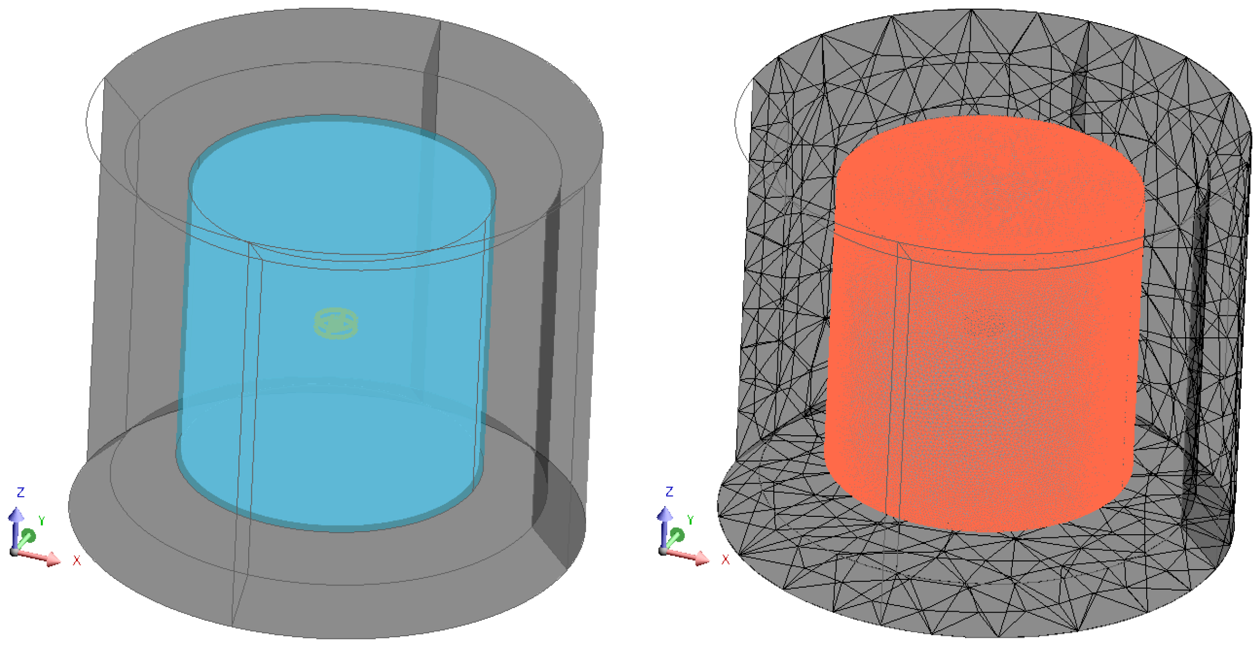
3.3. Numerical Model

In order to estimate the remanent magnetization (B_r) of each studied permanent magnet, several numerical models with finite elements were made with the help of Altair Flux 3D software version 22.2.0. Since the numerical models and the boundary conditions are similar, only the case of the CRRM is presented below. The numerical model of the CRRM and the mesh distribution are shown in Figure 4. Its geometric dimensions are mentioned in Figure 1a.

Figure 4. The numerical model of the permanent magnet and the mesh distribution.

In order to maintain a density of nodes as high as possible, the domain was divided into two subdomains; thus, in the blue volume, Figure 5, a much higher density of nodes was used compared to the volumes outside it. Following the application of the 2nd order mesh distribution, a total number of nodes of over 4.9 × 10⁶ was obtained.

Figure 5. The domain and the mesh distribution of the model.

In the numerical model, the Infinite Box (the black domain in Figure 5) was used, so the field inside this domain is not influenced by the boundary conditions of the model.

Figure 6 shows the red line from which the magnetic field values were extracted; it includes 500 points and has the following coordinates: starting point (20,0,0) and end point (120,0,0) mm.

Figure 6. The magnetic field values were extracted from the red line.

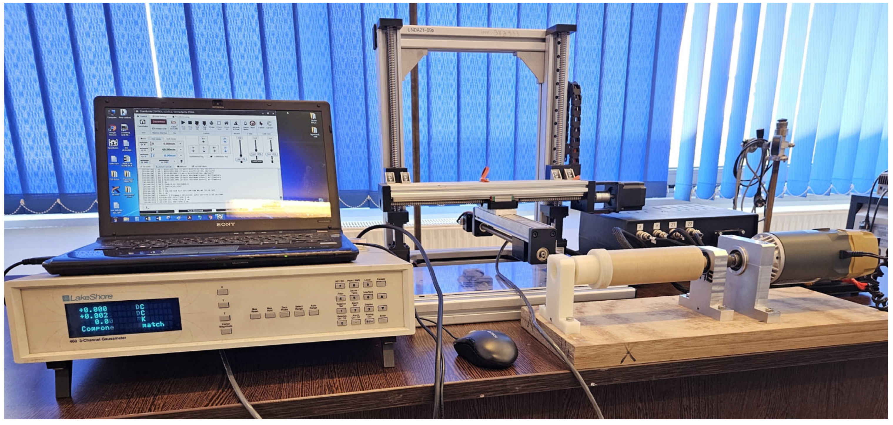
3.4. Measurement Setup and Equipment

Figure 7 presents the experimental setup that was used for measuring the static and dynamic magnetic field (70 Hz) generated by the two configurations versus distance, up to 100 mm.

Figure 7. Experimental setup used for measuring the static and dynamic magnetic field vs. distance between 2 and 100 mm.

The equipment presented in Figure 7 are given in Table 2.

Table 2. Equipment used for measuring the magnetic field vs. distance.

LakeShore Hall Probe Model MMZ-2508-UH (Lake Shore Cryotronics, Inc., Westerville, OH, USA)	LakeShore 460 Gaussmeter (Lake Shore Cryotronics, Inc., Westerville, OH, USA)	Multi Axis Positioning System
Frequency range: DC and 10 Hz, to 400 Hz	Frequency range: DC and 10 Hz, to 400 Hz	Three axis of coordinated motion
Operating temperature: 10 °C to 40 °C	DC accuracy: ±0.10% of reading ±0.005% of range	Resolution: 0.1 mm
Accuracy (% of reading at 25 °C): 0.25% from 0 to 20 kG; 0.5% from 20 kG to 30 kG;	DC temperature coefficient: ±0.05% of reading ±0.003% of range per °C	USB computer interface
Temperature coefficient: ±0.09 G/°C	AC RMS accuracy: ±2% of reading (50 to 60 Hz);
	AC peak accuracy: ±5% typical

For determining harmonics and interharmonics, the experimental setup shown in Figure 8 was used.

Figure 8. Experimental setup for determining harmonics and interharmonics for the two configurations of rotating permanent magnet antennas in an anechoic chamber.

It can be seen from the figure above that the two sensors used for measuring the magnetic field were symmetrically placed about the rotating magnet. The characteristics of these sensors are given in Table 3.

Table 3. The field sensors used for measuring the magnetic field generated by the rotating magnets.

Narda EHP-50F	Magnetic Sensor Coil
Frequency range: 1 Hz–400 kHz	38,000 turns;
Measurement domain (B): 0.3 nT–10 mT	Resistance (R): 7.2 kΩ
Dynamic range: >105 dB	Inductance (L) = 236.8 H @ 1.6 Hz
Dimensions: 92 mm × 92 mm × 109 mm	Medium diameter: 160 mm
Software: EHP50-TS	Made in house

The magnetic field received by the Narda EHP-50F sensor (Narda Safety Test Solutions GmbH, Pfullingen, Germany) is displayed on a laptop by means of the specialized software, and the signal given by the magnetic sensor coil is received with the spectrum analyzer embedded in a Tektronix MSO58 oscilloscope (Tektronix, Inc., Beaverton, OR, USA).

In order to determine the variation of magnetic field with distance in the case of the CRRM, between 1 m and 25 m, as well as for determining the maximum distance at which the signal generated by the rotating magnet can be detected in a suburban environment where the 50 Hz component is less than 1 nT, the same field sensors mentioned in Table 3 were used; for measuring the signal given by the magnetic sensor coil, a Rohde&Schwarz NF-Geräuschspannungsmesser Psophometer UPGS microvoltmeter was used (frequency range 15 Hz–20 kHz, sensitivity 1 µV; Rohde & Schwarz GmbH & Co. KG, Munich, Germany).

4. Results

4.1. Numerical Results

For the CRRM studied in steady state (static regime), several values of the remanent magnetization were considered: B_r = {1; 1.05; 1.1; 1.17; 1.21} T and a relative permeability μ_r = 1.0446. The dependence of the magnetic field induction with the distance is presented in Figure 9 for the values obtained from the numerical models (the dashed lines) as well as for the values (red line) measured by using the experimental setup in Figure 7. The variation of the magnetic field induction over the range 0–100 mm is shown in the top graph and that over the range 50–100 mm is shown in the bottom graph.

Figure 9. The dependence of the magnetic field induction with the distance, obtained in steady state for the CRRM, (a) over the range 0–100 mm and (b) over the range 50–100 mm.

The values obtained with the help of the numerical models were selected and compared with those obtained experimentally; thus, the relative errors and the root mean square deviation were determined (Figure 10).

Figure 10. (a) The relative errors obtained after comparing the values obtained numerically and those obtained experimentally; (b) the root mean square deviation.

As can be seen, the smallest differences are obtained in the case of the remanent magnetization value of B_r = 1.17 T. For the interval 0–80 mm, the relative errors have values below 5%; after this interval, they reach values of 6.98% and 8.45%.

The numerical model for the CABM is similar to the one presented above; only the geometry of the permanent magnet has been modified. After applying the 2nd order mesh distribution, a total number of nodes of over 4.4 × 10⁶ was obtained.

For the CABM studied in steady state (static regime), several values of the remanent magnetization were considered: B_r = {1; 1.05; 1.1; 1.17; 1.21} T and a relative permeability μ_r = 1.0446. The dependence of the magnetic field induction with the distance is presented in Figure 11 for the values obtained from the numerical models (the dashed lines) as well as for the values (red line) measured by using the experimental setup in Figure 7. The variation of the magnetic field induction over the range 0–100 mm is shown in the top graph and that over the range 50–100 mm is shown in the bottom graph.

Figure 11. The dependence of the magnetic field induction with the distance, obtained in steady state for the CABM, (a) over the range 0–100 mm and (b) over the range 50–100 mm.

The values obtained with the help of the numerical models were selected and compared with those obtained experimentally; thus, the relative errors and the root mean square deviation were determined (Figure 12).

Figure 12. (a) The relative errors obtained after comparing the values obtained numerically and those obtained experimentally; (b) the root mean square deviation.

As can be seen in Figure 12, the smallest differences are obtained in the case of the remanent magnetization value of B_r = 1.21 T. For the interval 5–60 mm, the relative errors have values below 5%.

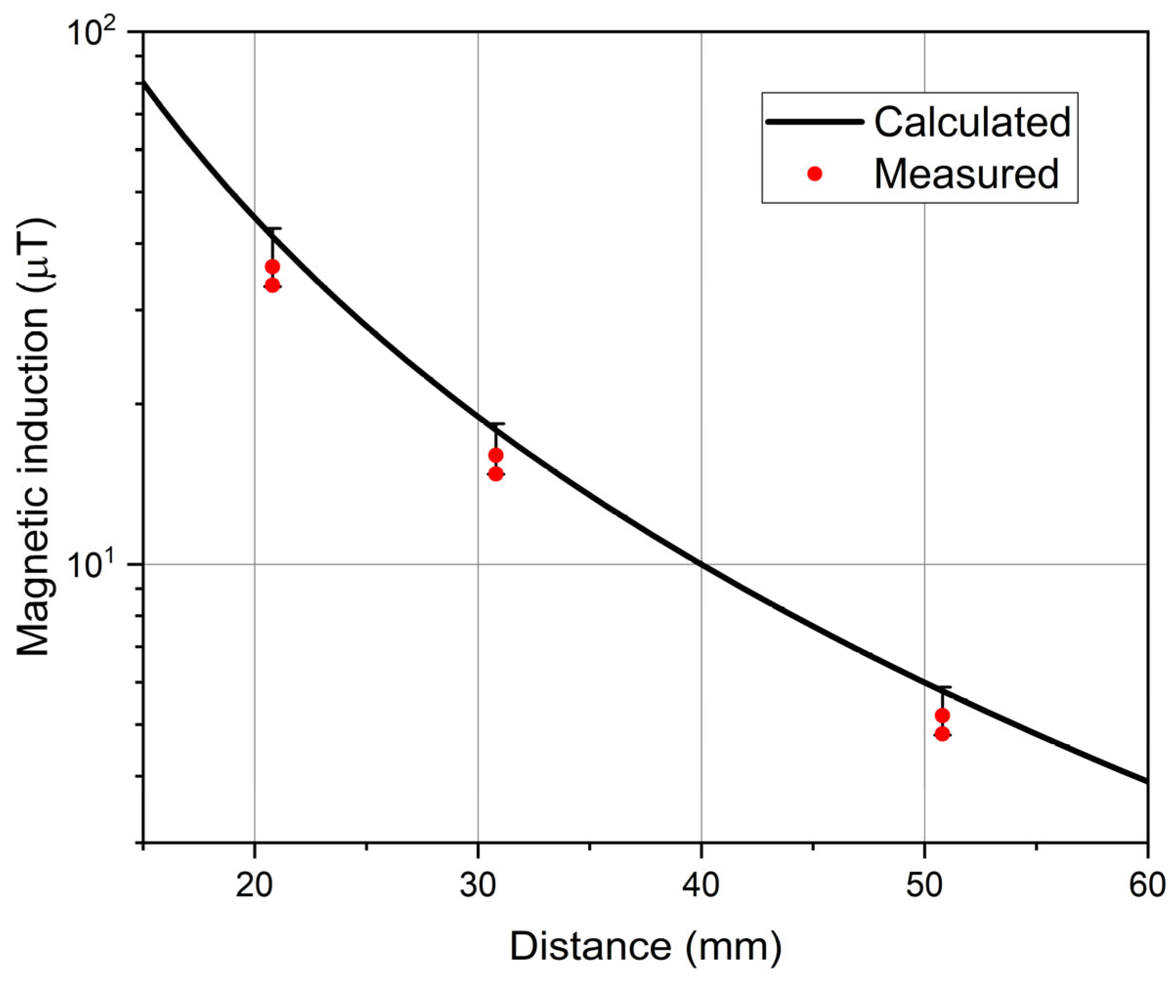
4.2. Experimental Results up to 100 mm

The dependence of the magnetic field generated by the two rotating magnet configurations on distance was measured up to 100 mm in the laboratory by using the multi-axis positioning system and a gaussmeter with a Hall probe (setup in Figure 7).

4.2.1. Mechanical Antenna with CRRM

Figure 13 presents the experimental results for the mechanical antenna with CRRM.

Figure 13. Magnetic field values in static and dynamic (70 Hz) regimes obtained for the CRRM between 2 and 100 mm.

A very good agreement between the values measured in static regime and the one measured in the dynamic case is observed, with the maximum difference being less than 3.16% up to 90 mm.

4.2.2. Mechanical Antenna with CABM

The measurement results obtained in static and dynamic regimes (70Hz) for the CABM are presented in Figure 14. In addition, because, for this case, there is an analytical equation that can be easily calculated, namely Equation (2), the calculated curve for the magnetic field emitted by the CABM was drawn (the black curve in Figure 14). In this case, the maximum percentage differences are as follows: static-calculated 30.3%, dynamic-calculated 14.8%, and measured dynamic-static 19.2%.

Figure 14. The magnetic field generated by the CABM, measured in static and dynamic (70 Hz) regimes between 2 and 100 mm; comparison with the values calculated using Equation (2).

4.3. 1/r³ Dependence and the Maximum Receiving Distance of Magnetic Field in a Suburban Environment

The magnetic field measurements in a suburban environment at a frequency of 70 Hz were made only with the CRRM using the house-made magnetic sensor coil with the Rohde&Schwarz UPGS microvoltmeter and Narda field sensor with the characteristics mentioned in Table 3. Table 4 below shows the magnitude of the received signal in mV and µT, the ratio of these quantities, and 1/r³ curves for the two types of measurements. Because of its lower sensitivity, the Narda sensor was only used for measurements up to 10 m. The noise level in the suburban area was around 10 μV.

Table 4. Magnetic field level measured in an environment with a low 50 Hz component.

Distance [m]	Voltmeter [mV]	Narda Sensor [µT]	Ratio mV/µT	1/r3 [mV]	1/r3 [µT]
1	320	1.2385	258.38	320	1.2385
2	40	0.1478	270.64	40	0.154813
3	12	0.0449	267.26	11.85	0.04587
4	5.2	0.0203	256.16	5	0.019352
5	2.4	0.0089	269.66	2.56	0.009908
10	0.32	0.0012	266.67	0.32	0.001239
15	0.08			0.095	0.000367
20	0.02			0.04	0.000155
25	0.005			0.02	7.93 × 10−5

Except for the column containing the ratio between the values measured with the mentioned equipment, Table 4 give the four dependencies plotted in Figure 15.

Figure 15. Variation of the transmitted magnetic field with distance at 70 Hz between 1 m and 25 m and 1/r³ dependence.

The last two values were obtained by subtracting the noise value from the measured value. This explains the relatively large errors at 20 and 25 m.

4.4. The Equivalence Between the Magnetic Field Emitted by the Rotating Magnet Relative to the Field Produced by Coils/Solenoid

First, the magnetic field generated by a solenoid with 50 turns carrying a current of 4 A at 70 Hz was measured. The solenoid has geometric dimensions similar to those of the CABM (L = 50 mm, R = 4 mm). The measurements were performed at three distances by using the Hall probe presented in Table 2. The obtained values (minimum and maximum values from a set of 10 measurements) are plotted in Figure 16 and compared with the theoretical values resulted from Equation (1) for the same characteristics of the solenoid.

Figure 16. Comparison between the theoretical and measured values of the magnetic field generated by a solenoid with 50 turns carrying a current of 4 A and having dimensions similar to those of the CABM.

These values can be found in Table 5 along with the values measured in the case of the CABM (same values in Figure 14). Also, Table 5 contains the ratios of these quantities for two cases: magnet (measured)–solenoid (theoretical) and magnet (measured)–solenoid (measured).

Table 5. Theoretical and measured values for the magnetic field generated by the CABM and solenoid.

	20 mm		30 mm		50 mm		100 mm
Solenoid (theoretical value)	41.22 µT		17.86 µT		5.99 µT		1.11 µT
Magnet (measured value)	9900 µT	9900 µT	4230 µT	4230 µT	1460 µT	1460 µT	270 µT
Solenoid (measured value)	34 µT	37.3 µT	14.8 µT	16 µT	4.9 µT	5.1 µT
Ratio: Magnet (measured)– Solenoid (theoretical)	240.17		236.84		243.74		243.24
Ratio: Magnet (measured)– Solenoid (measured)	291.18	265.42	285.81	264.38	297.96	286.27

On the other hand, we sought to make an equivalence between the magnetic field emitted by a rotating CRRM and the field generated by a coil-type circuit element. In this case, the dynamic field value emitted by the magnet at 70 Hz was compared with the values obtained with a coil whose characteristic data were found through a recurrent calculus using Equation (5) until a B = F(r) curve similar to that of the magnet was obtained (Figure 17). The following values were obtained for this coil: N = 5 turns, I = 1000 A, a = 22 mm.

Figure 17. Measurements performed in the dynamic regime and calculus for evaluating the equivalence between the magnetic field emitted by the mechanical antenna with a rotating CRRM and the magnetic field generated by a coil with a = 22 mm carrying a current I = 1000 A.

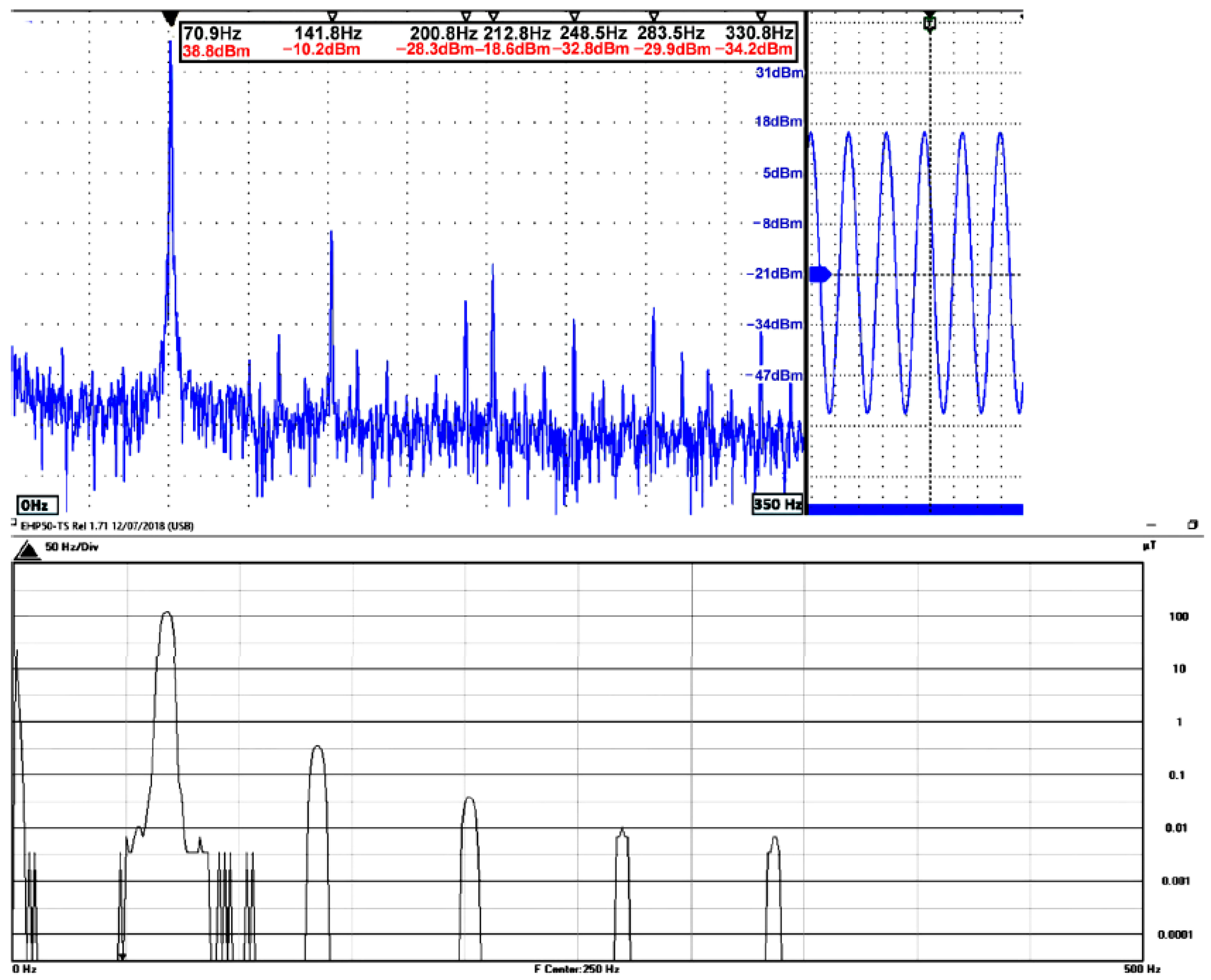
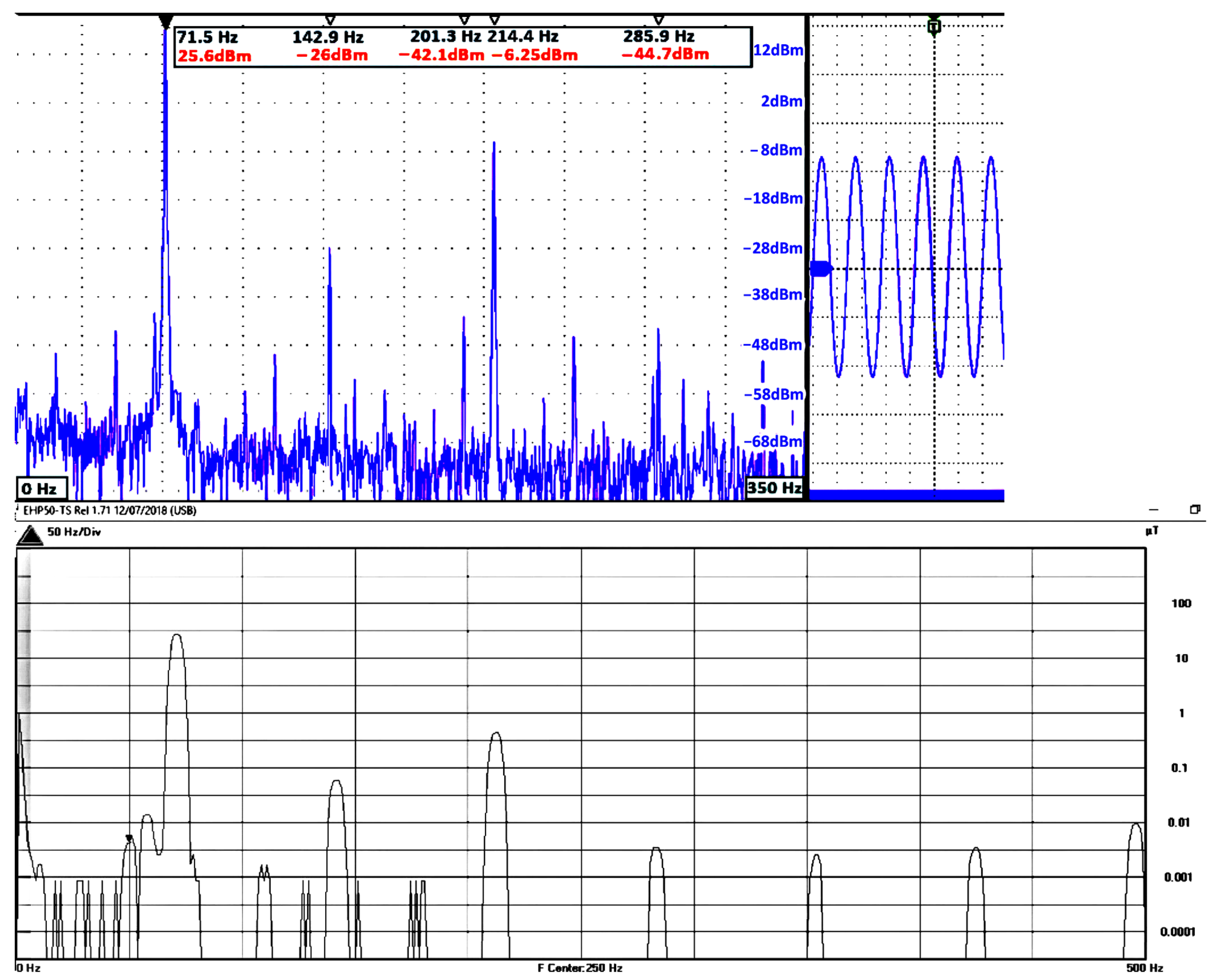
4.5. Harmonics and Interharmonics

For the harmonic analysis of the magnetic field generated by the two specified rotating magnet structures, the setup in Figure 8 was employed. The measurements were performed simultaneously with the two types of devices specified in Table 3. The obtained diagrams are shown in Figure 18 and Figure 19. The spectrum analyzer related to the oscilloscope Tektronix MSO58 displays the values in dBm, on the ordinate, specifying the frequency values for the fundamental and harmonics, while the Narda EHP-50F sensor software gives the values in μT.

Figure 18. The spectrograms obtained with the two devices (Narda sensor and magnetic sensor coil) for the CRRM.

Figure 19. The spectrograms obtained with the two devices (Narda sensor and magnetic sensor coil) for the CABM.

Table 6 synthesizes the values obtained in the above spectrograms and shows the calculated harmonics weight relative to the fundamental frequency.

Table 6. Values obtained in the harmonic analysis for the two types of rotating magnets.

Magnet Type	Units	Fundamental	2nd Harmonic	3rd Harmonic	4th Harmonic
CRRM	Hz	70.9	141.8	212.8	283.5
	dBm	38.8	−10.2	−18.6	−29.9
CABM	Hz	71.5	142.9	214.4	285.9
	dBm	25.6	−26	−6.25	−44.7
Harmonics weight relative to fundamental frequency
CRRM			49 dBm	57.4 dBm	68.7 dBm
			1/282	1/741	1/2690
CABM			51.6 dBm	31.85 dBm	70.3 dBm
			1/380	1/39	1/3162

5. Discussion and Conclusions

This article is based on a consistent bibliographic study in order to establish the current performances of mechanical antennas with rotating permanent magnets and to relate these performances to the experiments performed by the authors. The two mentioned configurations (CABM and CRRM) are employed, the latter proving to have better performance in all aspects.

Regarding the material, at this time, NdFeB permanent magnets are the most efficient. One of the competitors is the SmCo permanent magnet which has higher temperature stability and corrosion resistance but is economically uncompetitive at the moment.

The numerical results prove a good agreement between the numerical analysis and measurements: 5% error for the CRRM over the range 0–80 mm considering a remanent induction B_r = 1.17 T and 5% for the CABM over the range 5–60 mm considering a remanent induction B_r = 1.21 T.

In the next stage, we sought to establish to what extent the intensity of the emitted magnetic field presents differences between the static and the dynamic (harmonic) regimes.

Through these measurements, it was proven that the configuration with CRRM is superior from this point of view, with the maximum difference between the two regimes being of 3.16% while for the CABM, the differences are much bigger. For this last configuration, there is a simple analytical relationship—Equation (2)—used to calculate the magnetic field; therefore, in Figure 14, the theoretical curve was also drawn.

For a CRRM, there is no simple analytical relationship to calculate the magnetic field; the algorithm presented in [28,29] requires numerical calculation. Thus, in the case of the CRRM, it can be concluded that the static regime and the harmonic regime at a frequency of 70 Hz are quasi-identical in terms of the emitted field.

The analytical calculations and experimental results presented in the article highlight some aspects of novelty/originality relative to the research in the field so far:

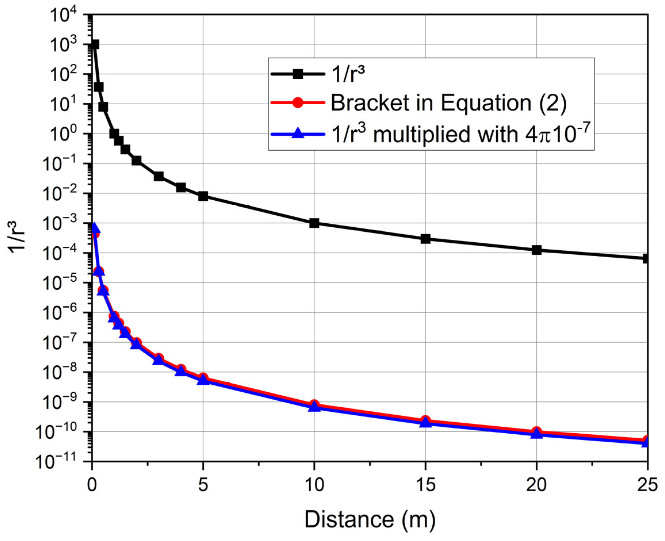
• The equivalence between relations (1) and (2) is a matter that has not been specified so far. Moreover, it is analytically demonstrated that the distance dependence of the magnetic field of these configurations scales as 1/r³. A similar approach, but without theoretical explanations, is attempted in [30].
• Demonstrating the 1/r³ dependence up to a distance of 15–20 m; in the studied bibliography, these distances are much smaller.
• Harmonic analysis via competing test methods (replicate testing), which was not found in the bibliography. This is of great importance in the analysis of the efficiency of these types of antennas.
• Experimental demonstration of the quasi-identity for the magnetic fields emitted as a function of distance in the static and harmonic regimes at the used frequencies. This assertion, together with the demonstration of the 1/r³ dependence, immediately leads to the idea that in order to evaluate the intensity of the harmonic magnetic field radiated at a certain distance, we do not have to rotate the magnet: it is enough to measure the intensity of the static field in the laboratory at short distances.

Thus, many articles declare the 1/r³ dependence for the harmonic field emitted by the rotating magnet, which is somewhat assumed to be true due to the analytical relations (mainly the similarity with the magnetic field of the elementary magnetic dipole, respectively the loop antenna in the near-field zone)—Equations (4) and (5). Figure 16 experimentally demonstrates this dependence through measurements performed in a suburban environment with low magnetic noise over the range 1–25 m. If, in Table 4, we consider the ratio mV/µT as being constant (258–269) down to the last row (25 m), where the lower sensitivity of the Narda sensor no longer allowed the measurement in µT units, it follows that the magnetic field measured in mV units corresponds to a magnetic field of approximately 20 pT at a frequency of 70 Hz. Because the sensor used in the measurements (the made-in-house coil with 38,000 turns) gives a signal that is proportional to frequency according to the magnetic induction law, it follows that for a higher frequency, for instance, 350 Hz, we can measure a magnetic field of approximately 4 pT. This value can be considered the sensitivity limit of the experimental setup used in the measurements (the made-in-house coil with 38,000 turns and Rohde&Schwarz microvoltmeter).

The harmonic analysis of the harmonic field generated by the two magnet configurations at a frequency of 70 Hz was performed by using the assembly presented in Figure 8 with two different pieces of equipment simultaneously within the replicate testing concept. For both magnet types, harmonics of second, third, and fourth order as well as interharmonics were detected. The highest harmonic in the case of the CRRM is the second harmonic, while in the case of the CABM, the third one is the highest. The CRRM proved to have a better performance in this test too, the second harmonic being approximately 282 times smaller than the level of the fundamental frequency, while for the CABM, the third harmonic is only 39 times smaller.

The analysis of the analytical relationships and the measurement results lead to two very important conclusions that were not sufficiently explained in the studied bibliography. The first conclusion is based on the following two assertions demonstrated in the article:

• The identity between the magnetic field intensities in static and harmonic regimes for the studied configurations;
• Both analytical and experimental demonstration of the 1/r³-distance dependence of the intensity of the emitted magnetic field.

From here, it follows that in order to evaluate the performance of a rotating magnet system (CRRM and CABM), a few measurements at different distances (cm, m) in static mode are sufficient. By applying the above assertions, we can evaluate the emitted magnetic field intensity at any distance for the given configurations. Moreover, we can also evaluate the emitted signal reception sensitivity with the devices mentioned in this article as having the minimum estimated values of 20 pT and 4 pT at 70 Hz and 350 Hz, respectively.

The second conclusion refers to the comparative analysis of the “efficiency” of the magnetic field generated by a rotating permanent magnet relative to the magnetic field generated by coils/solenoids. From Section 4.4 and Equation (3) results for NdFeb magnets, we find the following:

• In the case of a solenoid with dimensions similar to the ones of the CABM, we should apply a current of the order of 4 × (236… 298) A, as follows from Table 5. Obviously these are estimated values, but the order of magnitude is 1000 A;
• In the case of the CRRM, in order to equate the intensity of the magnetic field it generates, we should have a dimensionally comparable structure (coil with five turns and a radius of 22 mm) carrying a current of 1000 A (see Figure 17).

From here, it follows that, for similar dimensions, the rotating magnet has a much higher efficiency than the coil/solenoid. Obviously, by increasing the number of turns, the performance of the circuit elements can be significantly improved. At the same time, it must be taken into account that at low frequencies, the value of the coil resistance is much higher than the value of the inductive reactance, so that only a small part of the generator’s power is found in the produced magnetic field.

In conclusion, these devices have come to the attention of the scientific community in the last decade, with applications mainly in non-destructive defectoscopy, but more importantly in underwater communications. In order for this latter application to become competitive, it is necessary to increase the emission power (reception of the magnetic field at greater distances) and increase the emission frequency. Increasing the emission power can be achieved by increasing the size of the permanent magnet. By increasing the emission frequency, a double advantage would be achieved: extending the reception distance when this is done with a solenoid (based on the law of magnetic induction) and improving the modulation characteristics of the carrier for information transmission—the main purpose of this application.

Mechanical antennas based on rotating permanent magnets have, as shown in the bibliography, the advantage of relatively simple, compact constructions but may include limitations regarding the maximum speed of the drive motor, the size of the permanent magnet, centrifugal force, balancing problems, etc.

However, an alternative method of development exists. As we showed in the article, for comparative dimensions, a coil/solenoid is much less efficient. Thus, to equalize the permanent magnet in dynamic mode, the current through the coil should be 1000 A, which obviously represents a non-technical solution, primarily due to the appearance of losses by the Joule–Lenz effect. On the other hand, a superconducting coil would eliminate this disadvantage, and, in addition, it would offer the possibility of operating at higher frequencies, unlike a rotating magnet. This comparison can be the subject of future research.

A first qualitative evaluation for the performances of CRMM can be carried out in the laboratory via stationary magnetic field measurements for different sizes based on the conclusions of this article.

References

1. Gong, S.; Liu, Y.; Liu, Y. A rotating-magnet based mechanical antenna (RMBMA) for ELF-ULF wireless communication. Prog. Electromagn. Res. M 2018, 72, 125–133. [Google Scholar] [CrossRef]
2. Gołkowski, M.; Park, J.; Bittle, J.; Babaiahgari, B.; Rorrer, R.A.; Celinski, Z. Novel Mechanical Magnetic Shutter Antenna for ELF/VLF Radiation. In Proceedings of the 2018 IEEE International Symposium on Antennas and Propagation & USNC/URSI National Radio Science Meeting, Boston, MA, USA, 8–13 July 2018. [Google Scholar] [CrossRef]
3. Li, J.; Liu, Y.; Gao, S.J.; Li, M.; Wang, Y.Q.; Tu, M.J. Effect of process on the magnetic properties of bonded NdFeB magnet. J. Magn. Magn. Mater. 2006, 299, 195–204. [Google Scholar] [CrossRef]
4. Liu, W.; Zhang, F.; Sun, F.; Gong, Z.; Liu, X.; Fang, G. Radiation principle and spatial direct modulation method of a low frequency antenna based on rotating permanent magnet. Chin. J. Electron. 2022, 31, 674–682. [Google Scholar] [CrossRef]
5. Dong, Y.; Wu, J.; Zhang, X.; Xie, T. A novel dual-permanent-magnet mechanical antenna for pipeline robot localization and communication. Sensors 2023, 23, 3228. [Google Scholar] [CrossRef]
6. Prasad, S.; Tok, R.U.; Fereidoony, F.; Wang, Y.E.; Zhu, R.; Propst, A.; Bland, S. Magnetic Pendulum Arrays for Efficient ULF Transmission. Sci. Rep. 2019, 9, 13220. [Google Scholar] [CrossRef]
7. Yi, Q.; Li, N.; Zhang, J.; Sun, Z. A Rotating-Magnet Based Mechanical Antenna for VLF Communication. In Proceedings of the Seventh Asia International Symposium on Mechatronics, Hangzhou, China, 19–22 September 2019; Volume II, pp. 69–77, Part of LNEE 589. [Google Scholar] [CrossRef]
8. Bao, J.; Tian, Y.; Wang, Y.; Yi, Q.; Li, N. Research on mechanical antenna performance based on rotating permanent magnet triangle array. J. Phys. Conf. Ser. 2021, 1971, 012005. [Google Scholar] [CrossRef]
9. Guo, M.; Wen, X.; Yang, S.; Xu, J.; Pan, X.; Bi, K. Extremely-low frequency mechanical antenna based on vibrating permanent magnet. Eng. Sci. 2021, 16, 387–392. [Google Scholar] [CrossRef]
10. Thanalakshme, R.P.; Kanj, A.; Kim, J.; Wilken-Resman, E.; Jing, J.; Grinberg, I.H.; Bernhard, J.T.; Tawfick, S.; Bahl, G. Magneto-mechanical transmitters for ultra-Low frequency near-field communication. arXiv 2021. [Google Scholar] [CrossRef]
11. Thanalakshme, R.P.; Kanj, A.; Kim, J.; Wilken-Resman, E.; Jing, J.; Grinberg, I.H.; Bernhard, J.T.; Tawfick, S.; Bahl, G. Magneto-mechanical transmitters for ultra-low frequency near-field data transfer. IEEE Trans. Antennas Propag. 2022, 70, 3710–3722. [Google Scholar] [CrossRef]
12. Zhang, W.; Cao, Z.; Wang, X.; Quan, X.; Sun, M. Design, array, and test of super-low-frequency mechanical antenna based on permanent magnet. IEEE Trans. Antennas Propag. 2023, 71, 2321–2329. [Google Scholar] [CrossRef]
13. Wu, H.; Jiang, T.; Liu, Z.; Fu, S.; Cheng, J.; You, H.; Jiao, J.; Bichurin, M.; Sokolov, O.; Ivanov, S.; et al. Magneto-mechano-electric antenna for portable VLF transmission. Adv. Electron. Mater. 2023, 9, 2300096. [Google Scholar] [CrossRef]
14. Niu, Y.; Ren, H. Transceiving signals by mechanical resonance: A low frequency (LF) magnetoelectric mechanical antenna pair with integrated DC magnetic bias. arXiv 2021. [Google Scholar] [CrossRef]
15. Fawole, O.C.; Tabib-Azar, M. An electromechanically modulated permanent magnet antenna for wireless communication in harsh electromagnetic environments. IEEE Trans. Antennas Propag. 2017, 65, 6927–6936. [Google Scholar] [CrossRef]
16. Burch, H.C.; Garraud, A.; Mitchell, M.F.; Moore, R.C.; Arnold, D.P. Experimental generation of ELF radio signals using a rotating magnet. IEEE Trans. Antennas Propag. 2018, 66, 6265–6272. [Google Scholar] [CrossRef]
17. Strachen, N.; Booske, J.; Behdad, N. A mechanically based magneto-inductive transmitter with electrically modulated reluctance. PLoS ONE 2018, 13, e0199934. [Google Scholar] [CrossRef] [PubMed]
18. Hosseini-Fahraji, A.; Manteghi, M.; Ngo, K.D.T. New way of generating electromagnetic waves. IEEE Trans. Antennas Propag. 2021, 69, 6383–6390. [Google Scholar] [CrossRef]
19. Toujun, Z.; Bao, W.; Xu, Z.; Zhao, M.; Huang, X.; Wei, W.; Liu, R.; Xie, G. Optimizing microstructure, magnetic properties and mechanical properties of sintered NdFeB magnet by double alloy method and grain boundary diffusion. Intermetallics 2023, 162, 108027. [Google Scholar] [CrossRef]
20. Brown, D.N. Fabrication, Processing Technologies, and New Advances for RE-Fe-B Magnets. IEEE Trans. Magn. 2016, 52, 2101209. [Google Scholar] [CrossRef]
21. Hioki, K. High performance hot-deformed Nd-Fe-B magnets (Review). Sci. Technol. Adv. Mater. 2021, 22, 72–84. [Google Scholar] [CrossRef]
22. NdFeB Magnets, Quadrant. Available online: https://www.quadrant.us/resources/Data-Sheet/1740.html (accessed on 25 September 2024).
23. Physics Forum. Available online: https://www.physicsforums.com/threads/formula-of-solenoid-magnetic-b-field-at-ending-middle-and-outside.828426/ (accessed on 22 October 2024).
24. Camacho, J.M.; Sosa, V. Alternative method to calculate the magnetic field of permanent magnets with azimuthal symmetry. Rev. Mex. Fis. E 2013, 59, 8–17. Available online: http://www.redalyc.org/articulo.oa?id=57048158002 (accessed on 12 August 2024).
25. Kaufman, A.; Itskovich, G. Quasistationary Field of Magnetic Dipole in a Uniform Medium. In Basic Principles of Induction Logging–Electromagnetic Methods in Borehole Geophysics; Kaufman, A., Itskovich, G., Eds.; Elsevier: Amsterdam, The Netherlands, 2017; pp. 163–172. [Google Scholar] [CrossRef]
26. Bădic, M.; Pîslaru-Dănescu, L.; Ștefan, M. Bazele Ecranarii Electromagnetice (Fundamentals of Electromagnetic Shielding); Electra Publishing House: Bucharest, Romania, 2007; Volume 1, pp. 33–34. ISBN 978-973-7728-93-7. [Google Scholar]
27. NYU Physics Department. Available online: https://physics.nyu.edu/~physlab/GenPhysI_PhysII/Intro_experimental_physicsII_write_ups/Magnetic-field-circular-coil_01_30_2017.pdf (accessed on 4 October 2024).
28. Nguyen, V.T.; Lu, T.-F. Analytical Expression of the Magnetic Field Created by a Permanent Magnet with Diametrical Magnetization. Prog. Electromagn. Res. C 2018, 87, 163–174. [Google Scholar] [CrossRef]
29. Ravaud, R.; Lemarquand, G.; Lemarquand, V.; Depollier, C.L. Analytical Calculation of the Magnetic Field Created by Permanent-Magnet Rings. IEEE Trans. Magn. 2008, 44, 1982–1989. [Google Scholar] [CrossRef]
30. Sun, F.; Zhang, F.; Ma, X.; Gong, Z.; Ji, Y.; Fang, G. Research on Ultra-Low-Frequency Communication Based on the Rotating Shutter Antenna. Electronics 2022, 11, 596. [Google Scholar] [CrossRef]
Disclaimer/Publisher’s Note: The statements, opinions and data contained in all publications are solely those of the individual author(s) and contributor(s) and not of MDPI and/or the editor(s). MDPI and/or the editor(s) disclaim responsibility for any injury to people or property resulting from any ideas, methods, instructions or products referred to in the content.
Article Metrics
Citations
Article Access Statistics
Multiple requests from the same IP address are counted as one view.