Classification of Real-World Objects Using Supervised ML-Assisted Polarimetry: Cost/Benefit Analysis

Abstract

We study the problem of classification of various real-world objects using as input a database (DB) of laboratory polarimetric measures (Mueller matrix elements—MMEs). It can work as a complementary technology of surroundings’ imaging that can be used, in particular, in autonomous driving. To this end, we look for an algorithm using less input parameters without great loss of the quality of classification. We start by analyzing the data in order to understand the attributes that are more important for associating the objects with one of several predefined classes. Different sets of attributes are studied using an artificial neural network (ANN), which is optimized in terms of the number of hidden layers and the activation function. After that, an improved machine learning (ML) architecture is built using the K-nearest neighbors (KNN) classifier on each cluster generated by applying the pre-trained ANN to the training set. This article focuses on the situation wherein one may not be able to measure all MMEs or it would be too expensive or challenging to implement when the measurement time is crucial. The results obtained for a reduced set of attributes using different ML architectures are very good, especially for the proposed combined ANN-KNN approach (wherein the ANN acts as a predictor and KNN as a corrector), which can help to avoid measuring all MMEs.

1. Introduction

The problem of obtaining essential information about remote objects and using it for detection and computer-assisted classification of objects into predefined groups arises in different contexts of utmost importance [1,2]. In particular, driving in complex traffic environments or hazardous conditions (night or heavy rain, for instance) would benefit from the computational assistance tools to reduce the risk and help the driver to take the right decision [3]. Other vital applications are detection of forest fires [4] and classification of atmospheric aerosols and clouds [5].

One of the critical issues concerns the detection of surrounding objects and their characteristics’ determination. The detection using electromagnetic waves scattered by the object, which can be loosely termed as optical sensing, is one of the most powerful approaches because, in addition to the detection of the object’s presence and measuring the distance to it and its relative velocity, this can bring some additional information, which can be used for its classification. This information is encoded in the variation of the optical signal intensity with the radiation wavelength (spectroscopy) or in the polarization states of the detected light (polarimetry). Unfortunately, the interaction of light with real-world objects is usually too complex to be described by solvable models and phenomenological approaches are the only feasible alternative.

In this article, we analyze a number of machine learning (ML) techniques for object detection and classification, which can be relevant in the context of autonomous driving. We aim at classifying real-world objects (in particular, in the context of autonomous driving) using polarimetric optical sensing data. The physical information about a remote object is provided by the polarimetry of the optical signal caused by the diffuse scattering of light from the object, a powerful method of remote sensing [6]. The polarization state of an optical beam interacting with matter may be changed by varying amplitudes, relative phase of orthogonal field components, or by its degree of polarization [7,8,9]. The approach we adopt is based on the Stokes–Mueller formalism [10]. The Stokes vector describes the state of polarization of any light beam, whereas the Mueller matrix (MM), consisting of 4 × 4 real elements, provides information related to the samples. The advantage of this approach with respect to the Jones calculus is that it can describe partially polarized or incoherent light. Polarimetric imaging and sensing methods have been applied to the detection of pollution in the atmosphere [5] or land slides in forested areas [11], and to the classification of materials [7,8,9]. Using extensive laboratory polarimetry measurements, described in our previous work [9], a database of several thousands of samples was built, wherein each sample (event) is characterized by 15 Mueller matrix elements (MMEs) normalized by the zeroth element, $M_{00}$, plus the angle of incidence (AoI) of the testing light beam onto the object’s surface. Some examples of the MME images are shown in Figure 1. Each sample in the DB was labeled according to one of seven different object classes (see Section 2).

Machine learning (ML) and, in particular, deep learning methods are widely used for the classification of objects and living beings [1,2,12,13,14]. Within a supervised ML approach, a reference database is used to build a classifier with the objective to associate new events with one of previously defined groups or clusters using information derived from the experiment. A wide range of machine learning techniques have already been employed in the context of autonomous driving [12]. These techniques include K-nearest neighbors (KNN), first introduced in Ref. [15]; support vector machines (SVMs), introduced in Ref. [16]; decision trees (DTs) [17,18,19] and their extension named random forest (RF) [20]; and artificial neural networks (ANNs), first introduced by [21]. An example involving KNN and SVM can be found in Ref. [22], where these techniques were implemented to validate the classification of the driver behavior regarding safe/unsafe stopping at junctions when the yellow light is on. In Ref. [23], the authors proposed an explicit DT approach for automated driving on a two-lane highway. Cichosz et al. [24] presented vehicle control algorithms in order to simulate a racing car control adopting imitation learning, using DTs and RFs. The use of ANNs in the context of autonomous driving has been considered by Kumar et al. [25], where a self-driving car using ANNs and computer vision is able to detect lanes, traffic light, and avoid frontal collision. The authors of Ref. [3] focused on pedestrian and vehicle detection in autonomous cars. In Ref. [26], the authors presented an overview of machine learning/deep learning algorithms in the context of autonomous driving architectures. More recently [27], another comprehensive survey of ML techniques applied in the context of autonomous driving was presented. Applications of ML methods for classification, recognition, or tracking of objects, living beings or phenomena in other contexts are described in recent reviews [1,2,4,13,28].

Combining the polarimetric imaging with ML algorithms becomes a popular approach [7,8,9,29,30,31,32,33], often applied in but not limited to the context of autonomous driving. In an earlier work by our group [9], it was described how support vector machines and artificial neural networks are used for object classification in the context of autonomous driving. The data on the urban objects to classify are obtained by means of the Stokes–Mueller polarimetry, wherein the MMEs are evaluated. However, obtaining all MMEs may be technologically difficult and/or too expensive for practical use. In particular, it may be problematic to implement the part related to circular polarizations in a portable polarimeter. Therefore, here we analyze how the success of classification varies with the amount of input information (number of considered MMEs), for classifiers based on different ML algorithms. We propose an ANN-KNN classifier, which can be a compromise between the classification accuracy and cost.

The remainder of this article is organized as follows. In Section 2, we provide some details on the data from the polarimetry setup and the features we use to create a robust classifier. We also analyze the data in order to identify the attributes that are essential for classifying the objects correctly, even though redundancy may help to achieve better results. Section 3 is dedicated to the ML architectures and their deployment within the object identification context. Here we compare classification results obtained with different sets of attributes (minimal, intermediate, and full) and propose the ANN-KNN classifier. Finally, Section 4 presents a brief summary, conclusions, and outlook.

2. Materials and Methods

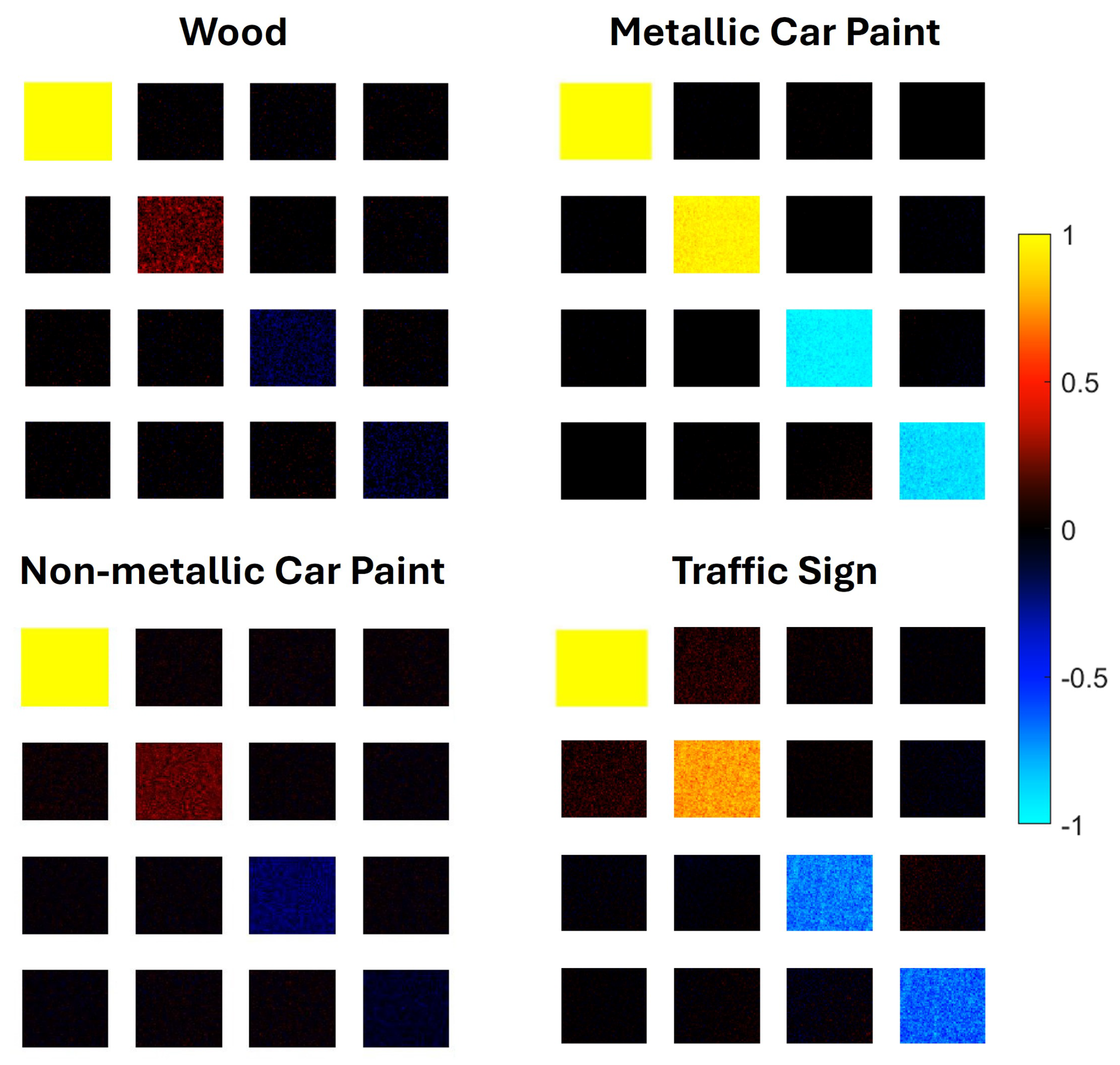
2.1. Data Collection

The detection of remote objects and collection of the data to be used in their classification is achieved by using the complete MM polarimeter described in Ref. [9]. The measurements were performed under conditions close to backscattering, with a small angle ($\approx 9^{\circ }$) between the illumination and detection arms of the setup [9]. The polarimetric database used in the present work contains the MMEs of the objects/materials listed in

Table 1. Classes of objects/materials considered.

Number, i	1	2	3	4	5	6	7
Description	Usual (solid) car paint	Car paint with metal flakes	Clothes (cotton, polyester, viscose, etc.)	Tree leaves	Granite stones used in pavements	Traffic signs (front side)	Tree trunk pieces
Short name	carP-C	carP-M	clothes	leaves	rocks	traf. sign	wood

.

The four-component Stokes vector, $\overrightarrow{S}$, describes the state of polarization of any light beam, no matter whether it is fully or partially polarized and coherent or not [10]. Its components are real parameters, which can be expressed as quadratic forms of the electric field amplitudes corresponding to different polarizations, either linear or circular. An arbitrary light scattering process can be described by the relation

$${\overrightarrow{S}}_o=\widehat{M}{\overrightarrow{S}}_i$$

(1)

where ${\overrightarrow{S}}_i$ and ${\overrightarrow{S}}_o$ are the Stokes vectors of the incident and outgoing beams, respectively, and $\widehat{M}$ stands for the Mueller matrix, which contains information regarding the polarizing/depolarizing properties of the sample. In general, it requires 16 independent measurements made with a polarimetric setup to determine the full MM. Under backscattering conditions, it has certain symmetry properties, which reduce the number of independent MMEs to 10 or even to 9 if it is considered normalized by the element $M_{00}$ as it usually is the case [6]. Nevertheless, it can be useful to retain some redundancy, which can compensate for measurement errors.

The information received from the polarimeter is processed to obtain the Mueller matrix elements, at a given AoI (denoted by $\alpha$) (The angle of incidence is known in laboratory measurements, while it can be determined using the triangulation method employing the parallax effect in non-laboratory situations. It can strongly influence the state of polarization of the backscattered light, especially for grazing incidence [11]). The polarimetric measurement matrix principle followed to calculate any Mueller matrix was described in detail elsewhere [10]. Summarizing the method, according to Equation (1) one needs to relate the input and output Stokes vectors, which are determined by the polarization state generator (PSG) and polarization state analyzer (PSA). Therefore, combining different PSG and PSA configurations, the matrix of intensities measured by the camera, $\widehat{B}$, can be written as

$$\widehat{B}=\widehat{A}\widehat{M}\widehat{G},$$

(2)

where the columns in the matrix $\widehat{G}$ correspond to the Stokes vectors generated by the PSG and $\widehat{A}$ is a matrix whose rows contain the different configurations used by the PSA. The Mueller matrix is calculated by selecting one of the relevant PSG-PSA configuration combinations, measuring the respective intensity and then solving Equation (2) at each pixel. It yields a map such as that shown in Figure 1.

Complete Mueller–Stokes polarimetry requires at least 16 measurements per data point which is difficult in a non-laboratory scenario. If we abdicate measuring the retardance, the number of measurements per data point can be reduced. By using only linear polarizations, the device has the potential to be more compact, affordable, and faster compared to a complete polarimeter. Two particular cases of interest are explored in this work:

(i)

Only two linear polarizations (horizontal and vertical) are used in both PSG and PSA; four measurements per data point are performed yielding the MMEs $M_{00}$, $M_{01}$, $M_{10}$, and $M_{11}$.

(ii)

Multiple angles are used for the linear polarizers in both PSG and PSA, so that at least nine measurements per data point are performed resulting in the MMEs listed in (i) plus $M_{02}\dots M_{22}$.

In order to create a dataset, we obtain a list of events (samples) of the form $\mathbf{e}=(\overrightarrow{x},\overrightarrow{y})$, where $\overrightarrow{x}=(x1,x2,...,x16)$ gathers the attributes, namely the MMEs are normalized by $M_{00}$, while the last parameter $x16$ is the angle of incidence. Vector $\overrightarrow{y}=\{y1,y2,...,y7\}$ with the entries being 0 or 1, attributed according to the following convention: $y1$—metallic car paint, $y2$—usual car paint, $y3$—clothes, $y4$—tree leaves, $y5$—rocks, $y6$—traffic signs, and $y7$—wood (see Table 1). The dataset for learning and test purposes was composed of 4000 samples, each of them with its $\overrightarrow{x}$. We denote by $D=\{e1,e2,...,eN\}$ the complete list of N = 28,000 events $\mathbf{e}$ and we split it into two sets, one for training the classifier (with 80% of the samples of the dataset), and a second one (the remaining 20% of the samples) to test the classifier.

2.2. Statistical Analysis of Input Attributes

A simple statistical analysis was carried out in order to obtain an insight about the main characteristics of the dataset and potential correlations or dimensional reduction. We calculated the mean values (“avg”) and the standard deviations (“std”) for each MME, for a given material label. We introduced the coefficients of variation, a ratio matrix, $CV$, between the standard deviation and the corresponding mean value. These parameters are used to define whether an attribute brings relevant information or not [34]. The $CV$ entry $(i,j)$ of a MME $M_{ij}$, for a given material m and an AoI $\alpha$ is given by

$${\displaystyle C{V}_{ij}^{m,\alpha }=lo{g}_{10}\frac{std\left(M_{ij}^{m,\alpha }\right)}{\left|avg\right(M_{ij}^{m,\alpha }\left)\right|}.}$$

(3)

Positive $CV$ values indicate uncertainty, which means that the information entry may not be conclusive. On the contrary, a high signal-to-noise ratio corresponds to a negative $CV$ value, which can be used as a criterion to select the most relevant Muller matrix elements for classification. Figure 2 shows the $CV$ parameters for four MMEs, for each of the 7 classes studied.

From Figure 2 we can see that the above criterion is always fulfilled for $M_{11}$. It also applies to the other diagonal MMEs, which means that they are the most robust attributes for classification algorithms. As expected, the absolute values of $CV<0$ are maximal for the most regular objects (samples of car paints and traffic signs) and they peak at $\alpha =0$, which corresponds to specular reflection. On the other hand, the criterion $CV<0$ is almost never fulfilled in the case of $M_{02}$, which means that considering $M_{02}$ as an attribute for a ML algorithm will probably not provide much reliable additional information. Other non-diagonal components have also been analyzed using this criterion and, generally, appear less relevant than the diagonal ones. This can be due to the fact that their mean values (for some classes of materials) are close to zero because these materials almost do not polarize, diattenuate, or introduce retardance. However, the case of $M_{01}$ and $M_{10}$ shown in the bottom panels of Figure 2 is intermediate, since most of the materials partially convert linearly polarized light into orthogonal polarization, as exemplified by the well-known cases of metal and dielectric spheres [35].

By analyzing the full set of 15 normalized MMEs, we verified that the attributes that present the best $CV$ ratios are $M_{11}$, $M_{22}$, $M_{33}$, $M_{01}$, and $M_{10}$, and these can be regarded as the most relevant attributes. Even though one should theoretically expect $M_{01}=M_{10}$ under backscattering conditions by virtue of the reciprocity theorem [6], in practice they are not equal (as are different their statistical $CV$-s in Figure 2), in part because of deviations from the strict backscatterting conditions even in laboratory measurements, beyond the inevitable measurement errors. Moreover, as mentioned above, retaining more information, despite its partial redundancy and low signal-to-noise ratio characteristic of some measured MMEs, may be helpful in ML algorithms. We will show evidence of this in the next section, although it should be seen from the cost/benefit point of view.

3. ML Architectures and Results

According to the earlier study [9], an artificial neural network is a reliable ML algorithm for this type of classification problem. We started by exploring the use of random forest (RF) classifiers using Matlab built-in functions [36] as an alternative to ANNs, but the average accuracy obtained was lower than when using ANNs. So, we decided not to follow this route to build our classifier and focused on ANNs. Yet, for the sake of completeness, we present the results obtained with the RF algorithm (Section 3.1).

ANN-based classifiers were considered with cross-validation, which was achieved by using the function fitcnet generating different ANNs. For this, we fixed 80% of the entire dataset as a training set and 20% as a testing set. The output of the function provides the best ANN according to the options “OptimizeHyperparameters”, setting “MaxObjectiveEvaluations” equal to 100. The hyperparameters taken into account included the maximum number of objective functions evaluated, the activation function, and layer sizes.

Below, we present the results obtained for different sets of attributes with random forest and the optimized ANN. We verified that ANNs indeed produce better results that RF. This study proceeded with ANNs as basis for our classifier. We also verified that, at some variance with the conclusion of Ref. [9], the angle of incidence is an important attribute, especially if we use less attributes as input for the ANN. This can be understood from the physical point of view for well-polished surfaces (such as car paint samples), which are characterized by strong specular reflection. So, we included the AoI even in the reduced set of MME attributes.

We also propose an ML architecture based on the ANN and the K-nearest neighbors (KNN) classification algorithm [37]. It consists in three steps. First, an ANN classifier is built by using the fitcnet function on the training dataset. Secondly, using the dataset on the ANN classifier, seven clusters are built, one for each class of objects obtained from the ANN, but keeping the original label. Finally, for each of the seven clusters, a KNN classifier is built (the best value of K is chosen by using the Matlab function fitcknn), allowing for an improvement in the success ratio for some classes when a reduced number of attributes is used. This approach is further explained in Section 3.4 of this paper.

3.1. RFs with Different Sets of Input Attributes

Our first approach was based on the random forest algorithm. RF classifiers have the advantage of the decision being easier to track than with an ANN and the training is computationally less expensive. However, we verified that the accuracy obtained is lower than when using an ANN. An RF is a collection of decision trees, generated from a subset of the training set. In the decision process, all the trees are consulted and the classification is made via a democratic count of votes. The Matlab function that makes it possible to build a random forest is called TreeBagger. In our simulations, we considered an RF with 200 trees and the in-bag fraction considered was 50%. This is the fraction of input data to sample with replacement from the input data for growing each new tree.

Below, we present our results for different sets of attributes.

• Attributes $M_{01}$, $M_{10}$, and $M_{11}$.
  The results obtained with these attributes are shown in Figure 3. Considering only MMEs $M_{01}$, $M_{10}$ and $M_{11}$, the overall classification accuracy obtained with the optimized ANN is 72.4%. It is easily seen that some classes are poorly identified, which means that the number of attributes is insufficient.
• Attributes $M_{01}$, $M_{02}$, $M_{10}$$M_{11}$, $M_{12}$, $M_{20}$, $M_{21}$, and $M_{22}$.
  Considering these eight MMEs as attributes, the overall classification accuracy obtained with the optimized ANN is 88.1% (we do not present the confusion table for brevity). The results are much better than with the minimal set, but the classes “leaves” and “rocks” are still not well distinguished.
• All MMEs as attributes.
  The results obtained with the complete set of attributes are shown in Figure 3 (right panel). Considering $M_{01}$, $M_{02}$, $M_{10}$$M_{11}$, $M_{12}$, $M_{20}$, $M_{21}$, and $M_{22}$ as attributes, the overall classification accuracy obtained with the optimized ANN is 93.85%. The accuracy obtained is now very good.

3.2. ANNs with Different Sets of Input Attributes

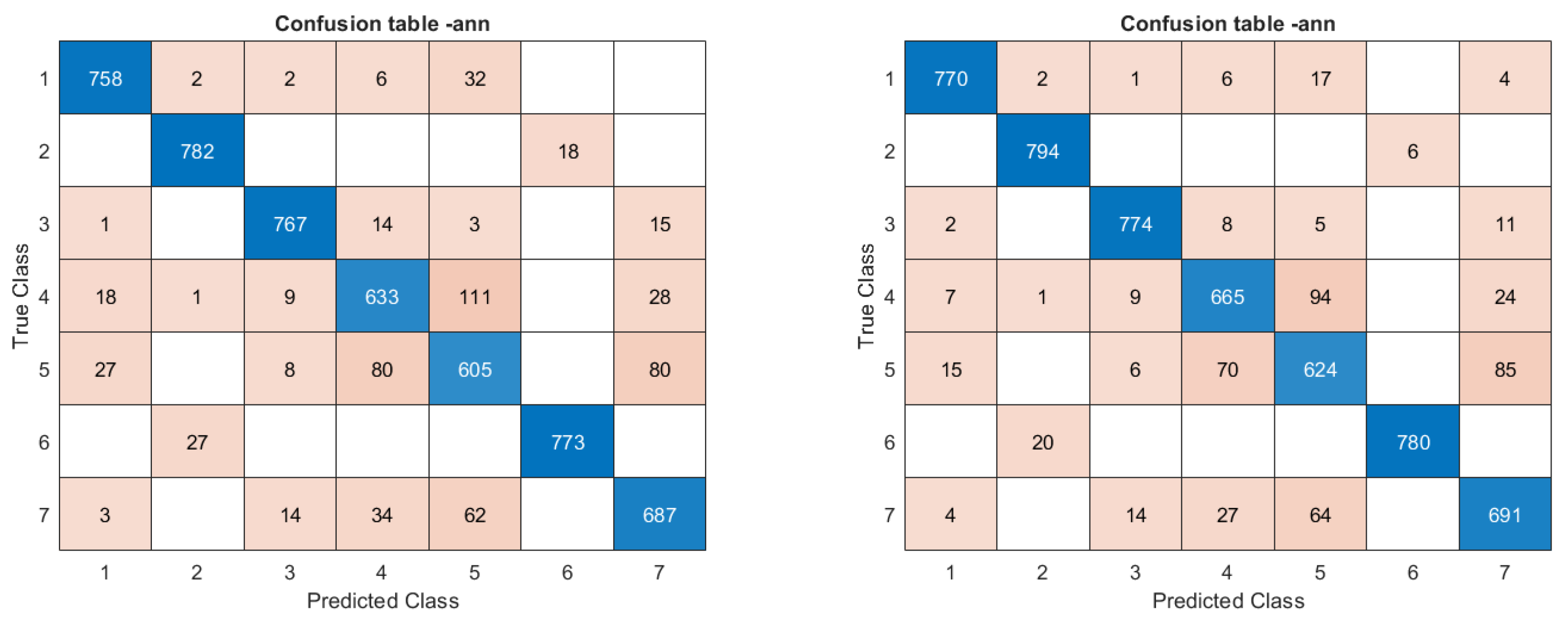
In this section, we analyze the influence of the set of attributes considered on the accuracy rate obtained by the optimized ANN classifier.

• Attributes $M_{01}$, $M_{10}$, and $M_{11}$ vs. $M_{01}$, $M_{10}$, and $M_{11}$ plus AoI.
  The results obtained with these attributes are shown in Figure 4. Considering only MMEs $M_{01}$, $M_{10}$, and $M_{11}$, the overall classification accuracy obtained with the optimized ANN is 74.14%. It is easily seen that some classes are poorly identified, which means that the number of attributes is not enough. However, the results are better than when using RF. By adding AoI to the list of attributes, the accuracy obtained raises to 77.28 % (see the right panel of Figure 4). Still, the classes “leaves”, “rocks”, and “wood” present rather poor rates of success with these sets of input parameters.
• Attributes $M_{01}$, $M_{02}$, $M_{10}$$M_{11}$, $M_{12}$, $M_{20}$, $M_{21}$, $M_{22}$ vs. $M_{01}$, $M_{02}$, $M_{10}$$M_{11}$, $M_{12}$, $M_{20}$, $M_{21}$, $M_{22}$ plus AoI.
  By using as attributes just the MMEs $M_{01}$, $M_{02}$, $M_{10}$$M_{11}$, $M_{12}$, $M_{20}$, $M_{21}$, and $M_{22}$, the accuracy obtained is now 89.3% (Figure 5, right panel). The results are better than when using RF. The results are much better than with the minimal set, but the classes “leaves” and “rocks” are still not well distinguished. By adding the angle of incidence to the list of attributes, the accuracy obtained is now 91% (right panel). Once again, AoI appears to be an important input parameter.
• All MMEs plus AoI as attributes.
  With the full set of MMEs as attributes, the accuracy increases to 95.9% (see Figure 6), whereas with the angle of incidence added to the list it reaches 96.2%, a relatively small advantage in comparison with the other cases. We may understand it as being due to the fact that the compatibility of the not fully independent MME values already determines AoI implicitly. The numbers obtained here are very similar to those quoted in Ref. [9], also obtained with the full set of MMEs but with a slightly different database and definition of classes.

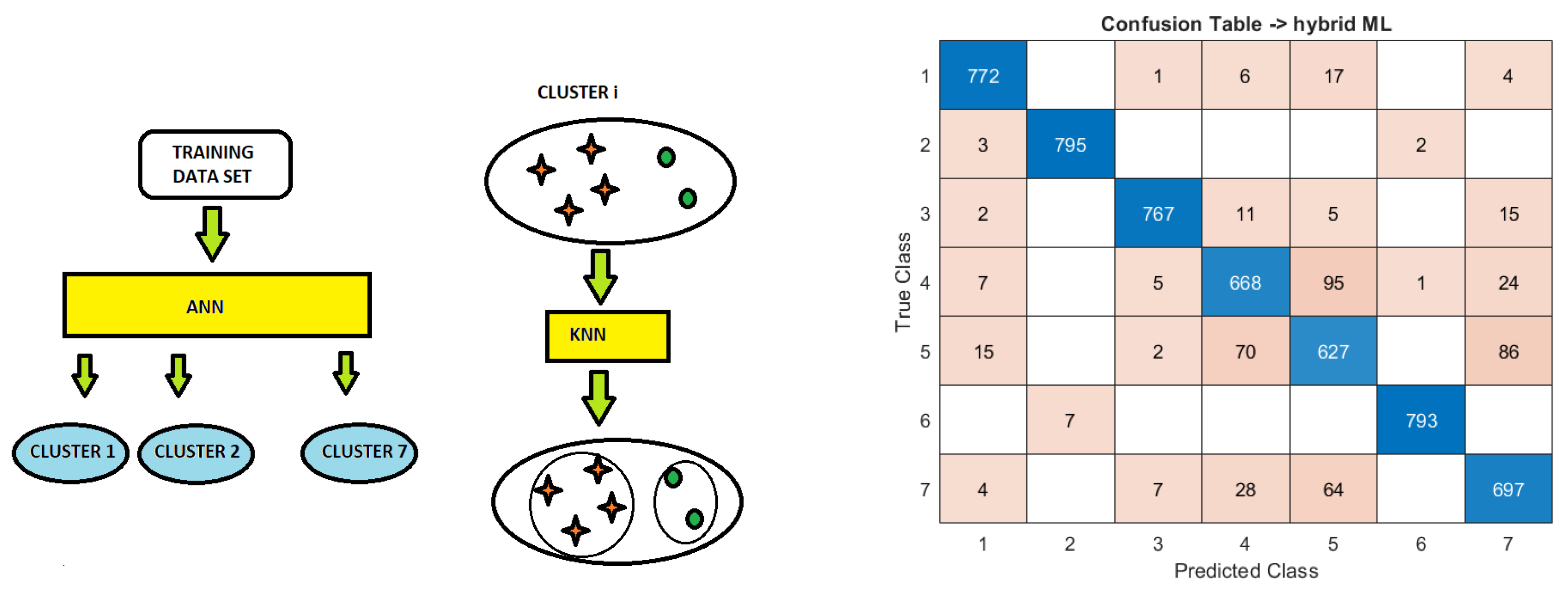
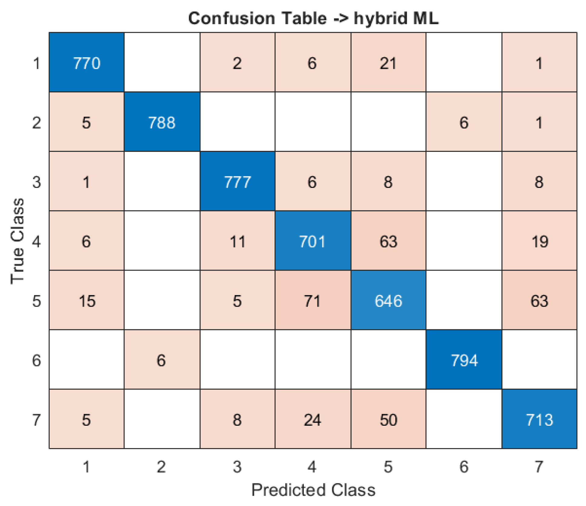
3.3. ANN-KNN Classifier

Here, we shall consider the intermediate set of attributes analyzed in the previous section, namely the MMEs $M_{01}$, $M_{02}$, $M_{10}$$M_{11}$, $M_{12}$, $M_{20}$, $M_{21}$, $M_{22}$ plus AoI, which can be a compromise between the accuracy and technological cost because it does not involve circular polarizations. We will show that the ML algorithm based on ANNs can be improved by combining it with the KNN algorithm.

Suppose that the optimized ANN has been generated from the training set by employing the Matlab fitcnet function. We define seven clusters, one for each class obtained by applying the trained ANN to all samples in the training DB. Notice that, in reality, some of the samples in the same cluster were misclassified and belong to a different class (see Figure 7, left panel). Then, for each of these clusters, a KNN classifier is built (the best value of K is chosen by using Matlab function fitcknn), which enables us to discriminate some of the misclassified objects because the true class of each object in the training DB is known (see Figure 7, central panel). So, there are at least some clusters for which the KNN reclassifies some of the misclassified samples (while the majority have been classified correctly by the ANN).

At the testing stage, each new event is an input for the ANN classifier. It falls in a cluster from 1 to 7. Then, the KNN classifier for that cluster is activated and the event is reclassified. It can retain the same classification or may change it. This correcting procedure of the classification is achieved. This methodology acts as a predictor corrector classifier, for which the ANN acts as a predictor and the KNN as a corrector.

The ANN-KNN classifier does improve the results obtained with the intermediate set of attributes, as can be seen from the confusion table shown in the right panel of Figure 7. The overall classification accuracy obtained raises to 91.4% if the angle of incidence is included. This represented an improvement of 0.4% is the accuracy rate, but it meant 4.4% less misclassifications.

It can be seen from the diagonal entries of the confusion table in Figure 7 that the most “problematic” classes are 4, 5, and 7. In order to remediate it, we considered another ML architecture with four additional attributes, which are internal products of the attribute vector of the sample, $\overrightarrow{x}$, with the average attribute vectors of class 3 (clothes) and the three problematic classes, $<\overline{x}{>}_i,i=3,4,5,7$ (the internal product involves only MMEs, not the AoI entry). These additional attributes are expected to emphasize the difference between these classes and they come without additional measurement cost.

We applied this algorithm to the same set of eight MMEs considered in this section, which yielded a total of 13 attributes. With the ANN-KNN approach, the accuracy of the classification results improved further, reaching 92.6% (see Figure 8). Although it is not as good as if we considered as attributes all 15 MMEs plus AoI, this ML architecture provides a very good overall accuracy rate at a considerably lower technological cost.

3.4. Recall Metric of Classifiers’ Performance

Beyond confusion tables, there are two performance metrics used in information retrieval, named Precision and Recall [38]. The latter, defined as

$${\displaystyle Recall=\frac{N\left(truepositive\right)}{N\left(truepositive\right)+N\left(falsenegative\right)},}$$

is complementary to the confusion table since it highlights the classification sensitivity. The number $N\left(falsenegative\right)$ is the sum of all non-diagonal element in the line of the confusion matrix, which corresponds to a certain class.

Table 2. Recall values for seven object classes calculated using ANN with 9 attributes, 8 MMEs + AoI.

Class	carP-C	carP-M	Clothes	Leaves	Rocks	Traf. Sign	Wood
Recall	96.2%	99.2%	96.7%	83.1%	78%	97.5%	86.3%

and

Table 3. Recall values for seven object classes calculated using ANN + KNN with 9 initial attributes and kernel.

Class	carP-C	carP-M	Clothes	Leaves	Rocks	Traf. Sign	Wood
Recall	96.2%	98.5%	97.1%	87.6%	80.8%	99.2%	89.1%

present the Recall values for each of the seven classes calculated for the results obtained with the ANN and ANN+KNN classifiers and the same set of nine initial input parameters (eight MMEs + AoI). In the case of ANN+KNN, the kernel was designed to emphasize the classes “clothes”, “leaves”, “rocks”, and “wood” by adding to the list of ANN inputs the corresponding $(\overrightarrow{x}·<\overline{x}{>}_i)$ as explained in Section 3.3. In other words, the the Recall values in two tables correspond to the data presented in Figure 5 and Figure 8, respectively. Comparing the two tables, we notice an overall improvement, while it is considerable for the most “problematic” classes, namely “leaves” and “wood”.

4. Discussion and Conclusions

We presented the results of our search for a machine learning architecture that could help to improve the classification of real-world objects, based on polarimetric data, in particular in the context of autonomous driving. They indicate that ANN-based architectures provide a slightly higher overall classification accuracy in comparison with the decision tree and random forest algorithms when applied to the full set of Mueller matrix elements. Taking into account earlier published results as well [9], we suggest that ANNs are preferable as supervised ML architectures for supporting this kind of sensing for classification. As shown in the previous work [9] and further confirmed in this study, an overall accuracy over 95% can be achieved, which is much higher than the values reported in Ref. [29] for deep learning-assisted 3D integral imaging, both polarimetric and non-polarimetric (It should be noticed that the data used in Ref. [29] were obtained in adverse environmental conditions, while ours were collected in laboratory).

However, the full Stokes–Mueller polarimetry may be too costly in the context of autonomous cars and, on the other hand, there are other sensing technologies, such as video cameras, LiDARS, and SONARs, which complement the surroundings’ imaging to make the autonomous driving feasible [39]. Here, we have shown that, even without using all MMEs as attributes, one can obtain reasonably good classification results. Then, it is a question of cost/benefit to optimize the input dataset. The minimal set of just three essential MMEs, which is equivalent to using just two orthogonal linear polarizations, already permits to distinguish different types of car paint [40] but it is insufficient to distinguish between objects characterized by entirely diffuse scattering. A good compromise is to consider as attributes the MMEs $M_{01}$, $M_{02}$, $M_{10}$$M_{11}$, $M_{12}$, $M_{20}$, $M_{21}$, $M_{22}$, plus AoI (It excludes the elements $M_{03}$, $M_{13}$, $M_{23}$, $M_{30}$, $M_{31}$, $M_{32}$, and $M_{33}$ related to circular polarizations). With this set of input parameters, the overall accuracy rate obtained was 91%, compared to 96.2% obtained with the full set of MMEs. We verified that the angle of incidence has an impact on the accuracy of the classifiers, especially if a reduced number of MME attributes are used by the classifier.

We developed a kernel approach with an ANN-KNN classifier (Figure 7), which employs the above set of MMEs and four new attributes defined as the internal product between the sample’s attribute vector and the average attribute vectors for the classes “clothes”, “tree leaves”, “rocks”, and “wood” in the training database. It yielded a further improved accuracy of 92.6% with the set of 13 attributes, of which only eight MMEs listed above and AoI have to be measured. This hybrid algorithm employing a kernel was shown to decrease the overall misclassification rate from 9% (using just ANN with eight MMEs + AoI) to 7.4% (an 18% reduction). As illustrated by the calculated Recall values, the reduction is more significant for the most “problematic” classes (“leaves” and “wood”). In the context of autonomous driving or, more generally, road scenes, the object class “clothes” is critical because its misclassifications can cause a disaster. In order to improve results for “clothes”, adding the object speed as a new attribute could be helpful since the speeds of people, cars, and other objects are usually quite different. This could come from the same or another sensor, e.g., a radar.

As another prospective application, such a ML architecture can be used in classifying problems in which sensors are based on spectroscopy; for instance, monitoring the environment-sensitive Localized Surface Plasmon Resonance (LSPR) in metallic nanoparticles [41], or on the detection of sound signals in metropolitan landscapes [42]. In the case of plasmonic sensors, polarimetry can also be tried for complementing and reducing the spectroscopy measurements while ML can help to detect small changes in the polarimetric response for certain wavelengths within the LSPR band.

References

1. Liu, L.; Ouyang, W.; Wang, X.; Fieguth, P.; Chen, J.; Liu, X.; Pietikäinen, M. Deep Learning for Generic Object Detection: A Survey. Int. J. Comput. Vis. 2020, 128, 261–318. [Google Scholar] [CrossRef]
2. Kaur, K.; Singh, S. A comprehensive review of object detection with deep learning. Digit. Signal Process. 2023, 132, 103812. [Google Scholar] [CrossRef]
3. Galvão, L.; Abbod, M.; Kalganova, T.; Palade, V.; Huda, N. Pedestrian and Vehicle Detection in Autonomous Vehicle Perception Systems—A Review. Sensors 2021, 21, 7267. [Google Scholar] [CrossRef] [PubMed]
4. Ghali, R.; Akhloufi, M.A. Deep Learning Approaches for Wildland Fires Remote Sensing: Classification, Detection, and Segmentation. Remote Sens. 2023, 15, 1821. [Google Scholar] [CrossRef]
5. Qi, S.; Huang, Z.; Ma, X.; Huang, J.; Zhou, T.; Zhang, S.; Dong, Q.; Bi, J.; Shi, J. Classification of atmospheric aerosols and clouds by use of dual-polarization lidar measurements. Opt. Express 2021, 29, 23461–23476. [Google Scholar] [CrossRef]
6. Cloude, S. Polarisation: Applications in Remote Sensing; Oxford University Press: Oxford, UK, 2009. [Google Scholar] [CrossRef]
7. Brown, J.P.; Roberts, R.G.; Card, D.C.; Saludez, C.L.; Keyser, C.X. Hybrid passive polarimetric imager and lidar combination for material classification. Opt. Eng. 2020, 59, 073106. [Google Scholar] [CrossRef]
8. Quéau, Y.; Leporcq, F.; Lechervy, A.; Alfalou, A. Learning to classify materials using Mueller imaging polarimetry. Fourteenth Int. Conf. Qual. Control. Artif. Vis. 2019, 11172, 246–252. [Google Scholar] [CrossRef]
9. Estevez, I.; Oliveira, F.; Braga-Fernandes, P.; Oliveira, M.; Rebouta, L.; Vasilevskiy, M. Urban objects classification using Mueller Matrix polarimetry and machine learning. Opt. Express 2022, 30, 28385–28400. [Google Scholar] [CrossRef]
10. Goldstein, D. Polarized Light; CRC Press: Boca Raton, FL, USA, 2014. [Google Scholar] [CrossRef]
11. Shibayama, T.; Yamaguchi, Y.; Yamada, H. Polarimetric Scattering Properties of landslides in Forested Areas and the Dependence on the Local Incident Angle. Remote Sens. 2015, 7, 15424–15442. [Google Scholar] [CrossRef]
12. Shaleb-Shwartz, S.; Ben-David, S. Understanding Machine Learning: From Theory to Algorithms; Cambridge University Press: Cambridge, UK, 2014. [Google Scholar] [CrossRef]
13. Ma, P.; Li, C.; Rahaman, M.M.; Yao, Y.; Zhang, J.; Zou, S.; Zhao, X.; Grzegorzek, M. A state-of-the-art survey of object detection techniques in microorganism image analysis: From classical methods to deep learning approaches. Artif. Intell. Rev. 2023, 56, 1627–1698. [Google Scholar] [CrossRef]
14. Mokayed, H.; Quan, T.Z.; Alkhaled, L.; Sivakumar, V. Real-Time Human Detection and Counting System Using Deep Learning Computer Vision Techniques. Artif. Intell. Appl. 2023, 1, 221–229. [Google Scholar] [CrossRef]
15. Fix, E.; Hodges, J. An Important Contribution to Nonparametric Discriminant Analysis and Density Estimation. Int. Stat. Rev. 1951, 57, 233–247. [Google Scholar] [CrossRef]
16. Vapnik, V.; Chervonenkis, A. On a class of algorithms of learning pattern recognition. Autom. Remote. Control 1964, 25, 838–845. [Google Scholar]
17. Quinlan, J. Induction of decision trees. Mach. Learn. 1986, 1, 81–106. [Google Scholar] [CrossRef]
18. Morgan, J.; Sonquist, S. Problems of analysis in survey data and a proposal. J. Am. Stat. Assoc. 1963, 58, 415–434. [Google Scholar] [CrossRef]
19. Hunt, E.; Marin, J.; Stone, P. Experiments in Induction; Academic: New York, NY, USA, 1966. [Google Scholar]
20. Ho, T. Random Decision Forests. In Proceedings of the 3rd International Conference on Document Analysis and Recognition, Montreal, QC, Canada, 14–16 August 1995. [Google Scholar] [CrossRef]
21. Rosenblatt, F. The Design of an Intelligent Automaton. Psychol. Rev. 1958, 65, 386–408. [Google Scholar] [CrossRef]
22. Karri, S.; De Silva, L.; Lai, C.; Yong, S. Classification and Prediction of Driving Behaviour at a Traffic Intersection Using SVM and KNN. SN Comput. Sci. 2021, 2, 209. [Google Scholar] [CrossRef]
23. Li, N.; Chen, H.; Kolmanovsky, I.; Girard, A. An Explicit Decision Tree Approach for Automated Driving. In Proceedings of the ASME 2017 Dynamic Systems and Control Conference, Tysons, VA, USA, 11–13 October 2017. [Google Scholar] [CrossRef]
24. Cichosz, P.; Pawelczak, L. Imitation learning of car driving skills with decision trees and random forests. Int. J. Appl. Math. Comput. Sci. 2014, 24, 579–597. [Google Scholar] [CrossRef]
25. Kumar, S.; Kumar, K.; Prakasha, G.; Teja, H. Self-Driving Car Using Neural Networks and Computer Vision. In Proceedings of the 2022 International Interdisciplinary Humanitarian Conference for Sustainability (IIHC), Bengaluru, India, 18–19 November 2022. [Google Scholar] [CrossRef]
26. Bachute, M.; Subhedar, J. Autonomous Driving Architectures: Insights of Machine Learning and Deep Learning Algorithms. Mach. Learn. Appl. 2021, 6, 100164. [Google Scholar] [CrossRef]
27. Zhao, J.; Zhao, W.; Wang, Z.; Zhang, W.; Zheng, W.; Cao, W.; Nan, J.; Lian, Y.; Burke, A. Autonomous driving system: A comprehensive survey. Expert Syst. Appl. 2024, 242, 122836. [Google Scholar] [CrossRef]
28. Meimetis, D.; Daramouskas, I.; Perikos, I.; Hatzilygeroudis, I. Real-time multiple object tracking using deep learning methods. Neural Comput. Appl. 2023, 35, 89–118. [Google Scholar] [CrossRef]
29. Usmani, K.; Krishnan, G.; O’Connor, T.; Javidi, B. Deep learning polarimetric three-dimensional integral imaging object recognition in adverse environmental conditions. Opt. Express 2021, 29, 12215–12228. [Google Scholar] [CrossRef] [PubMed]
30. Pierangeli, D.; Conti, C. Single-shot polarimetry of vector beams by supervised learning. Nat. Commun. 2023, 14, 1831. [Google Scholar] [CrossRef]
31. Makkithaya, K.N.; Melanthota, S.K.; Kistenev, Y.V.; Bykov, A.; Novikova, T.; Meglinski, I.; Mazumder, N. Machine Learning in Tissue Polarimetry. In Optical Polarimetric Modalities for Biomedical Research. Biological and Medical Physics, Biomedical Engineering; Mazumder, N., Kistenev, Y.V., Borisova, E., Prasada, K.S., Eds.; Springer: Berlin/Heidelberg, Germany, 2023. [Google Scholar] [CrossRef]
32. Rodríguez, C.; Estévez, I.; González-Arnay, E.; Campos, J.; Lizana, A. Optimizing the classification of biological tissues using machine learning models based on polarized data. J. Biophoton. 2023, 16, e202200308. [Google Scholar] [CrossRef]
33. Zhu, Z.; Li, X.; Zhai, J.; Hu, H. PODB: A learning-based polarimetric object detection benchmark for road scenes in adverse weather conditions. Inf. Fusion 2024, 108, 102385. [Google Scholar] [CrossRef]
34. Brown, C. Coefficient of Variation, Applied Multivariate Statistics in Geohydrology and Related Sciences; Springer: Berlin/Heidelberg, Germany, 1998. [Google Scholar] [CrossRef]
35. Born, M.; Wolf, E. Principles of Optics, 6th ed.; Pergamon Press: Oxford, UK, 1980; pp. 633–664. [Google Scholar]
36. MatLab Help Center. MathWorks. 2022. Available online: https://www.mathworks.com/help/stats/treebagger.html (accessed on 15 August 2024).
37. Steinbach, M.; Tan, P. kNN: K-Nearest Neighbors. In The Top Ten Algorithms in Data Mining; Chapman and Hall/CRC: Boca Raton, FL, USA, 2009. [Google Scholar] [CrossRef]
38. Precision and Recall. SciKit-Learn. 2024. Available online: https://scikit-learn.org/1.5/auto_examples/model_selection/plot_precision_recall.html (accessed on 1 November 2024).
39. Yeong, D.J.; Velasco-Hernandez, G.; Barry, J.; Walsh, J. Sensor and Sensor Fusion Technology in Autonomous Vehicles: A Review. Sensors 2021, 21, 2140. [Google Scholar] [CrossRef] [PubMed]
40. Nunes-Pereira, E.J.; Peixoto, H.; Teixeira, J.; Santos, J. Polarization-coded material classification in automotive LIDAR aiming at safer autonomous driving implementations. Appl. Opt. 2020, 59, 2530. Available online: https://opg.optica.org/ao/abstract.cfm?URI=ao-59-8-2530 (accessed on 22 November 2024). [CrossRef] [PubMed]
41. Rodrigues, M.; Borges, J.; Lopes, C.; Pereira, R.; Vasilevskiy, M.; Vaz, F. Gas Sensors Based on Localized Surface Plasmon Resonances: Synthesis of Oxide Films with Embedded Metal Nanoparticles, Theory and Simulation, and Sensitivity Enhancement Strategies. Appl. Sci. 2021, 11, 5388. [Google Scholar] [CrossRef]
42. Altayeva, A.; Omarov, N.; Tileubay, S.; Zhaksylyk, A.; Bazhikov, K.; Kambarov, D. Convolutional LSTM Network for Real-Time Impulsive Sound Detection and Classification in Urban Environments. Int. J. Adv. Comput. Sci. Appl. 2023, 14, 0141164. [Google Scholar] [CrossRef]
Figure 1. Normalized Mueller matrix images of some of the studied materials taken with 1550 nm radiation and AoI of 20 .
Applsci 14 11059 g001
Figure 2. Coefficients of variation for Mueller matrix elements M 11 (top left), M 02 (top right), M 01 (bottom left), and M 10 (bottom right) versus the angle of incidence for seven classes of materials/objects.
Applsci 14 11059 g002
Figure 3. Confusion table obtained using the RF algorithm with only M 01 , M 10 , and M 11 as attributes (left) and all 15 MMEs (right). AoI was included as attribute in both cases.
Applsci 14 11059 g003
Figure 4. Confusion tables obtained with only M 01 , M 10 , and M 11 as attributes (left) and with AoI added (right).
Applsci 14 11059 g004
Figure 5. Same as in Figure 4 but with MMEs M 01 , M 02 , M 10 M 11 , M 12 , M 20 , M 21 , and M 22 , without and with AoI.
Applsci 14 11059 g005
Figure 6. Same as in Figure 4 but with all 15 normalized MMEs, without and with AoI.
Applsci 14 11059 g006
Figure 7. ML architecture based on ANN + KNN (left and center) and its confusion table (right panel) where the attributes used are the same 8 MMEs as in Figure 5 plus the AoI (right).
Applsci 14 11059 g007
Figure 8. Confusion table for the ANN-KNN architecture with 13 attributes, which are the same 8 MMEs as in Figure 5, AoI, and 4 new attributes, ( x · < x ¯ > i ) , i = 3 , 4 , 5 , 7 .
Applsci 14 11059 g008